Snapshot Imaging of Stokes Vector Polarization Speckle in Turbid Optical Phantoms and In Vivo Tissues

Abstract

Significance: We present a system to measure and analyze the complete polarization state distribution of speckle patterns generated from in vivo tissue. Accurate measurement of polarization speckle requires both precise spatial registration and rapid polarization state acquisition. A unique measurement system must be designed to achieve accurate images of polarization speckle patterns for detailed investigation of the scattering properties of biological tissues in vivo. Aim and approach: This system features a polarization state analyzer with no moving parts. Two pixel-polarizer cameras allow for the instantaneous acquisition of the spatial Stokes vector distribution of polarization speckle patterns. System design and calibration methods are presented, and representative images from measurements on liquid phantoms (microsphere suspensions) and in vivo healthy and tumor murine models are demonstrated and discussed. Results and Conclusions: Quantitative measurements of polarization speckle from microsphere suspensions with controlled scattering coefficients demonstrate differences in speckle contrast, speckle size, and the degree of polarization. Measurements on in vivo murine skin and xenograft tumor tissue demonstrate the ability of the system to acquire snapshot polarization speckle images in living systems. The developed system can thus rapidly and accurately acquire polarization speckle images from different media in dynamic conditions such as in vivo tissue. This capability opens the potential for future detailed investigation of polarization speckle for in vivo biomedical applications.

1. Introduction

To meet the rising interest in speckle and its polarization properties for biomedical applications [1,2,3,4,5], this article details the creation of an optical probing system for snapshot in vivo measurements of the spatial polarization state distribution of polarization speckle. This system furthers developments in two fields of research with burgeoning applications in cancer detection: optical depolarization probing [6] and static speckle contrast analysis [1]. Both techniques measure properties of the stochastic interference pattern (“speckle pattern”) produced by laser light backscattering from in vivo tissue. Depolarization probing is a one-dimensional point-sensing measurement of the average polarization state of the backscattered light, lacking spatial resolution. Static speckle contrast yields spatially resolved information allowing for higher-order statistical analysis but has until now largely lacked polarization state information. Both were designed with clinical integration in mind, allowing for devices that are lightweight and portable, ultimately generating a single number for diagnostic use. The proposed polarization speckle system bridges the gap between the two and combines their parameter spaces to yield spatially resolved polarization state information of a speckle pattern from in vivo tissue. This system’s primary goal is to enable access to this expanded parameter space for greater potential tissue discrimination ability.

Speckle is a stochastic interference pattern of spatially varying coherent zones, often observed as a “salt-and-pepper” field of fluctuating intensities. It is created whenever coherent light is scattered from rough solid surfaces or turbid media (e.g., tissue), as cumulative phase differences are introduced into the wavefront. Speckle formation is currently understood as a random walk process [7]. Component phasors undergo random walks within the scattering medium, which results in a stochastic distribution of path lengths. The observed speckle pattern is the phasor sum at each point in space, consisting of zones of constructive and destructive interference. The term “polarization speckle” denotes that in any given speckle field, each illuminated point in space has a unique polarization state. The spatial fluctuations of these polarization states form a stochastic field of vectors in a similar manner to how speckle is regarded as a stochastic field of scalar intensities. In comparison to existing techniques, polarization speckle analysis involves both the addition of Stokes polarimetry to intensity-based speckle images, and an expansion of Stokes polarimetry to incorporate temporal and spatial coherence distributions.

The spatial inhomogeneity of polarization states within light fields has been recognized and studied for decades, with Goodman noting in 1976 that “the speckle patterns observed through a polarization analyzer will change detailed structure dramatically as the analyzer is rotated through 90°” [8]. Subsequent study on polarization heterogeneity in speckle patterns primarily focused on identifying the statistical distributions of Stokes parameters [9,10,11,12]. The term “polarization speckle” was used by Takeda’s group in 2009 [13] as they further described the statistical distributions of Stokes parameters in speckle. This term was adopted in the second edition of Goodman’s seminal textbook on speckle in 2020 [7]. Throughout this time, Amra et al. have demonstrated simulations and measurements of polarization speckle patterns from both surface scattering and bulk scattering [2,14,15,16]. Along with the evolving understanding of polarization speckle, data-driven approaches in optical polarization analysis are being explored [17], and similarly applied to polarization speckle [2]. Initial studies applying deep learning in speckle [18] and polarization speckle [3] illustrate how modern computational analysis methods are well suited to supporting and understanding speckle, as it is an information-rich stochastic signal that is otherwise unintuitive to interpret. The next step in polarization speckle research is to use this developed statistical understanding for applications in metrology. Specifically, polarization speckle applications in biomedicine are still in their early development.

Images of speckle patterns can be classified as objective or subjective, where objective refers to the interference pattern projected from the surface of a sample, and subjective refers to the pattern as it has been focused on a camera’s surface using a lens [8]. In this paper, we are exclusively concerned with objective speckle, to remove the influence of the lens on the speckle’s statistical properties and focus on the effects of scattering from the sample. The statistical properties of speckle can be observed from both a dynamic and a static perspective. The former describes how speckle fluctuates in time, subject to “boiling” as movement within the medium creates a blurring effect. An example of this principle is seen in laser speckle contrast imaging [19], which takes advantage of how motion in a medium relates to a reduction in speckle contrast due to blood flow. Recently, the polarization properties of dynamic speckle have been explored, finding enhancements to the technique both in polarization gating [20] and in parallel dynamic speckle plus Mueller matrix polarimetry measurements [21]. Static speckle refers to the spatial composition of the speckle pattern at a point in time, rather than its temporal progression. The contrast metric of static speckle patterns has been found useful in surface roughness measurement applications [22], and additional statistical metrics have been identified in these applications through machine learning [23]. The polarization properties of speckle and their connection to scattering medium properties has been initially explored in scattering phantoms [2] and has demonstrated utility in skin cancer diagnosis [1].

Thus far, studies have not investigated the parameter space offered by the complete Stokes vector distribution within static speckle from volume scattering. Accurate measurement of volumetric polarization speckles from tissue requires both precise registration of the spatial intensity fluctuations, and rapid polarization state measurement within the time frame of speckle’s temporal fluctuations. A unique measurement system must thus be designed to accurately study polarization speckle and explore the information provided on in vivo tissue. The reported system employs a combination of two pixel-polarization cameras to resolve the spatial Stokes vector distribution of polarization speckle (shortened to Stokes vector speckle) generated from in vivo biological tissue. This enables rapid polarization state measurement with no moving parts. Polarization speckle image visualization and analysis methods are presented on three types of testing media: an opaque metal surface, liquid microsphere suspensions, and an in vivo murine model. Initial reporting of first-order polarization speckle metrics from all media provides examples of this enhanced parameter space’s discrimination ability.

2. Background

2.1. Speckle Contrast and Size

As speckle patterns are stochastic phenomena, they can be described through statistical distributions. The intensity distribution generally follows a Gamma distribution, while the other Stokes parameters follow Laplace distributions [8,9,11]. In this paper, we use first-order statistical summary metrics to describe the relevant components of these speckle pattern statistics, with an investigation of higher-order statistical metrics to pursue in future studies.

Speckle contrast and speckle size are first-order metrics that can be used to infer the scattering properties of the medium that produced that speckle pattern [2,4,24]. Given a speckle pattern image represented by a 2D array of pixel intensities $I(x,y)$, speckle contrast is $C={\sigma }_I/〈I〉$, where σ_I is the standard deviation of intensity values and $〈I〉$ is the spatial average of intensity across the whole image. In the fully developed speckle pattern, which assumes sufficient scattering has occurred for the pattern to become fully ergodic, C = 1, which is generally the maximum value for observed speckle. Speckle contrast is notable for its use in surface roughness measurement [22,25]. Extending this to volume scattering, one expects that greater scattering turbidity decreases contrast, due to the wider resultant distribution of scattering pathlengths, as seen in experimental findings [24,26].

The speckle size (average speckle diameter) is calculated as the full-width half maximum of the speckle pattern’s normalized autocorrelation function [7]. In the fully developed case, speckle size is correlated to the illuminated area of the medium. In an opaque surface, this is the diameter of the illuminating laser [27], but in volume scattering, this “spot size” is the spatial extent of the exiting light on the surface of the illuminated object, which is correlated to turbidity and potentially other key scattering metrics of interest [2].

2.2. Polarization State and Degree of Polarization

This paper employs the Stokes vector convention to discuss the polarization state of light, chosen due to its ability to encode depolarization and ease of translation to the Poincaré sphere model, depicted in Figure 1A. In this model, the Stokes parameters S₁, S₂, and S₃ are the coordinate axes of a three-dimensional space, in which all polarization states exist within a sphere of unit radius 1 (the maximum magnitude) [28]. The magnitude of the vector is the degree of polarization (DOP), which spans [0, 1], where 0 indicates depolarized light and 1 indicates uniformly (100%) polarized light. Another way to interpret this is that 1 indicates light that is polarization coherent, and 0 indicates polarization incoherence. The degree of polarization is of great interest as a potential optical biomarker for cancerous tissue, notably as a conveyer of scattering angle differences between tissue types [6,29,30,31].

An important clarification for our purposes is that these conventions for polarization state and DOP are based on intensity measurements from a detector that employs both spatial and temporal integration. In speckle, the measurement of DOP (spatial polarization coherence) strongly depends on the window of pixels over which the polarization analysis is performed. This is due to the inhomogeneity of polarization states within multiply scattered speckle.

In Figure 1B, we introduce the visualization convention used throughout this paper to depict a spatial polarization state distribution. Each pixel is demarcated by a colored elliptical marker, where white markers indicate a primarily linear polarization state, cyan indicates right-hand helicity, and yellow indicates left-hand helicity. The size of the elliptical marker, indicated by the length of the major axis, is proportional to the DOP, with DOP = 1 being the largest. It is often the case that the polarization state at various pixels is relatively high and uniform, as seen in Figure 1B, where most markers exhibit similar size.

The DOP of each pixel is calculated as

$$DOP\left(n,m\right)={\displaystyle \frac{\sqrt{S_1{\left(n,m\right)}^2+S_2{\left(n,m\right)}^2+S_3{\left(n,m\right)}^2}}{S_0\left(n,m\right)}}$$

(1)

where n and m indicate the spatial coordinates of that pixel. For each n and m, there is a unique polarization state. For example, the Stokes vector of the pixel indicated in Figure 1B with a red box is [1; −0.43; 0.61; 0.35] and DOP(n,m) = 0.83. The Stokes vector of the green box is [1; −0.43; −0.27; −0.64] with DOP(n,m) = 0.82. For a statistical summary, we can determine the average of these individual pixel DOPs in a quantity named DOP_px. This is described as

$$DO{P}_{px}=\overline{DOP\left(n,m\right)}={\displaystyle \frac{\sum DOP\left(n,m\right)}{k_{px}}}$$

(2)

where k_px is the total number of pixels in the image. In Figure 1B, this averages to DOP_px = 0.88 (standard deviation = 0.17).

However, if this detector was a point-sensing photodiode of equivalent area rather than a camera, the average normalized Stokes vector would differ significantly. Wang et al. refer to this metric as the spatial degree of polarization (DOP_sp), though their definition assumes this parameter is calculated from a speckle field fully comprised of coherent and polarized points, rather than this computation from pixels that may be partially coherent and partially polarized [13]. To calculate this, we find the average Stokes parameters across the whole image and calculate the DOP_sp from these quantities:

$$\overline{S_1}={\displaystyle \frac{\sum S_1\left(n,m\right)}{k_{px}}} \overline{S_2}={\displaystyle \frac{\sum S_2\left(n,m\right)}{k_{px}}} \overline{S_3}={\displaystyle \frac{\sum S_3\left(n,m\right)}{k_{px}}}$$

(3)

$$DO{P}_{sp}={\displaystyle \frac{\sqrt{{\overline{S_1}}^2+{\overline{S_2}}^2+{\overline{S_3}}^2}}{\overline{S_0}}}$$

(4)

where k_px is the number of pixels being averaged. In Figure 1B, the average normalized Stokes vector of the whole image is [1; −0.24; 0.06; 0.22], resulting in DOP_sp = 0.33, a much lower value than DOP_px = 0.88. The ability to determine the distribution of DOP_px in addition to measuring the image-averaged DOP_sp significantly expands the explorable parameter space relative to the polarimetry and speckle approaches individually. We expect that access to these and other higher-order spatial polarization coherence metrics, alone or in combination with the spatial coherence metrics of speckle size and contrast discussed above, will allow for enhanced sensitivity and insight in measuring the volumetric scattering properties of biological tissues.

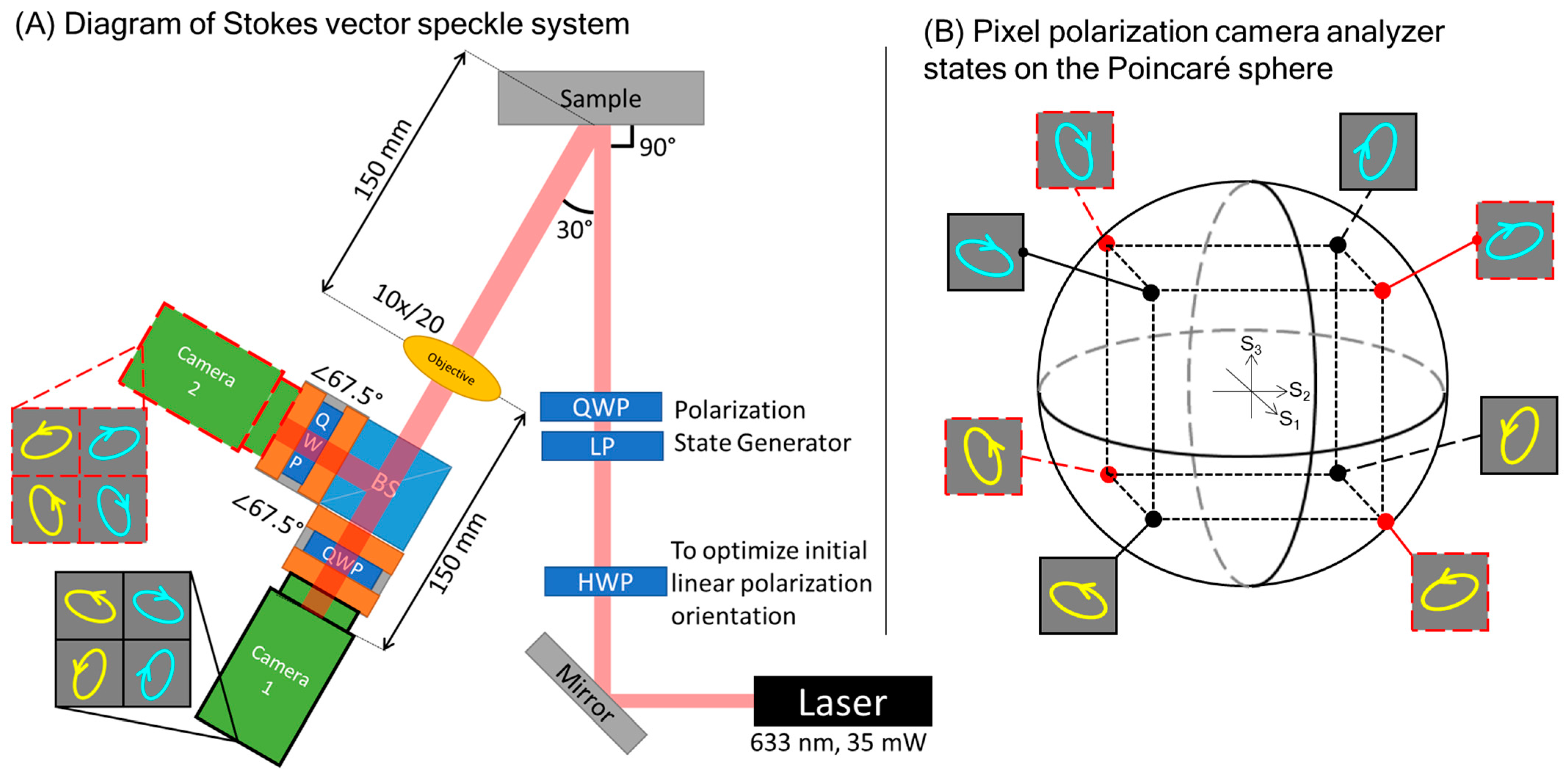
3. Methods—System Design

The purpose of this imaging system is to measure the objective speckle pattern backscattered from the illuminated sample; thus, the basic system schematic was composed of a laser directed at a scattering object, a camera system to receive the speckle pattern, and polarization-controlling components along the beam path to generate and analyze polarization states. A lens would not ordinarily be required, as the sample itself is not directly imaged by the system, but rather the diffuse scattered speckle pattern that was recorded on the camera’s surface. A magnifying objective was placed in the system only to increase the speckle size relative to the camera pixel size, as described in Section 3.1 below.

The primary challenge that this system was developed to overcome is that of polarization state measurement within the temporal rate of speckle fluctuations. In a medium with particle movement (such as Brownian motion, or a more regular convective flow), the speckle pattern will fluctuate and decorrelate in time, a phenomenon referred to as speckle boiling [7]. A long acquisition time will lead to smeared integration of speckles, which obscures accurate measurements. For the capture of speckle patterns in vivo, an acquisition speed below the rate of speckle boiling is required. In previous studies, we have estimated that for in vivo human tissue, this is a requirement below 5 ms [1]. However, for animal models with greater metabolisms, or phantoms with high flow rates, this requirement will become stricter.

The chosen detection scheme for the Stokes vector speckle device is a solid-state division-in-space polarization state analyzer (PSA) of two pixel-polarization cameras (PPCs) separated by a beam splitter, an advancement over previous devices [1]. This system is depicted in Figure 2A. The design emphasis has been placed on the PSA, as the major obstacle to overcome is polarization state measurement within temporal speckle fluctuations. This is necessary regardless of innovations in the polarization state generator (PSG). Furthermore, backscattering geometry is chosen due to its relevance to transmission for in vivo measurements in biomedical applications.

The illumination for the examples in this paper was provided by a HeNe laser (633 nm, 35 mW, JDS Uniphase). It should be noted that both the spatial and temporal coherence of a laser influence the generated speckle [32]; for the HeNe laser used here, the temporal coherence length is >200 mm based on interferometric measurement. A laser with a shorter temporal coherence will generate patterns with lower absolute contrast compared to a high-coherence gas laser [33], but it may show greater dynamic range in contrast between different media [34]. Future research will investigate how the coherence properties of the speckle system’s illumination can be optimized, as this paper focuses mainly on the ability to measure the polarization state distribution.

The PSA uses a non-polarizing beam splitter (Thorlabs CCM1-BS013), two quarter-wave plates, and two pixel-polarizer cameras (PPCs) (Lucid Vision Triton, Sony IMX250MZR CMOS). The beam splitter’s linear dichroism is compensated by the eigenvalue calibration process described in Section 3.3. The PPCs measure polarized light using clusters of four linearly polarized subpixels at 0°, 45°, 90°, and 135° linearly polarized angles. Two PPCs are required to capture a full Stokes vector once equipped with a quarter-wave plate each (Thorlabs WPQ10M-633). In Figure 2A and in subsequent discussion of this system, these PPCs are Camera 1, indicating the camera in the beam splitter transmission pathway, and Camera 2, for the camera in the beam splitter reflection pathway. A detection angle of 30° is used to avoid specular reflection and increase signal strength, as perpendicular measurement would require an additional beam splitter. As a related decision, the incident polarization state is right-hand circular throughout the demonstrations in this paper. The circular incidence is linearly symmetrical, minimizing the effect of the incidence angle creating asymmetry along a linear axis. Additionally, this geometry allows us to observe the helicity reversal caused by reflection.

From manufacturer specifications, the pixel-polarization cameras have a quantum efficiency of 45% and an extinction ratio of 145:1 at 633 nm. The cameras accommodate differences in quantum efficiency and wavelength dependence through manufacturer-provided software calibration. The total area of each camera detector is 2448 × 2048 subpixels (8445.6 µm × 7065.6 µm). The subpixels are 3.45 µm by 3.45 µm, resulting in a polarization superpixel size of 6.9 µm by 6.9 µm. Exposure time can be varied to adjust for signal strength, and in this study was kept to a maximum of 5 ms.

The images of Camera 1 and Camera 2 are registered using the feature-based registration technique SURF (Speeded Up Robust Features) deployed in MATLAB 2024. This registration is performed on the sum of all four channels, which results in an S₀ image approximation. The images of Camera 2 are left-right flipped prior to registration, to accommodate for the flip introduced by the beam splitter reflection. The two cameras’ images are each saved as a 4096 × 4896 pixel array of 8-bit values in the range of [0, 255]. These two images are separated into eight individual 2048 × 2448 polarization channel images, and then converted into floating point for pixel-by-pixel arithmetic operations.

3.1. Speckle Size Considerations

Using PPCs introduces spatial sampling discontinuity between subpixels of like polarization. To avoid information loss and minimize error caused by this, we require the speckle size of the pattern to be large relative to that of each superpixel of the PPC. This is comparable to requiring a high spatial sampling frequency to accurately record a spatial signal frequency. Using the Nyquist–Shannon sampling theorem as a guide, the minimum discrete spatial sampling frequency is twice the spatial signal sampling frequency. We can define the speckle spatial frequency as the inverse of speckle size. Put simply, one speckle must span at least two superpixels.

It is noted that in the imaging of subjective speckles, where a lens is applied to focus the sample image onto the camera, the speckle size is dependent on the lens aperture [7] [8]. Here, our system measures the objective speckle pattern and does not image the specimen but rather records the speckle pattern as it develops in free space. Specifically, the system images diverging speckles in the Fraunhofer zone as described by Gatti et al. [35]. In this case, the speckle size generated in a rough surface scattering scenario (opaque surface) can be calculated from the system geometry, incorporating the radius of backscattered light (or “spot size”), the illuminating wavelength and temporal coherence, and the distance between target and detector [7].

The diagonal of the 6.9 µm by 6.9 µm superpixel is 9.8 µm. Selecting this as the largest speckle detection dimension, we approximate our minimum-sized speckle as a circle with a diameter of 20 µm. System dimensions can be designed to ensure sufficient speckle size; however, volume scattering introduces further complexity, as in addition to currently unknown relationships, volume scattering generates a much larger spot size than the laser diameter due to dispersion of light. Our system employs a magnifying objective (Olympus WHK 10×/20, focal length = 25 mm, NA = 0.25) to ensure that the minimum dimension of the speckle is greater than the 20 µm minimum diameter.

Notably, the addition of a lens does not create an imaging configuration in this system, as the resulting focal plane is in the space 120 mm from the subject, rather than at the subject itself. In this way, the objective speckle pattern at that intermediate region of space is magnified onto the camera. Recognizing that the speckle may no longer be truly “objective” due to the addition of a lens, this method of speckle magnification should be investigated more closely in future study.

3.2. Polarimetric Scheme

Between the two pixel-polarizer cameras, the speckle pattern is split into eight constituent polarization states. In mathematical terms, a minimum of four independent polarization states are required to calculate a Stokes vector; however, from a practical standpoint, error can be reduced by using more than four detector states as these provide redundant measurements. To minimize error, the analyzer polarization states ought to be placed such that they maximize the volume they inscribe in the Poincaré sphere [36]. Error is further reduced by placing the detectors as far from the eigenstates (axes and equator) of the Poincaré sphere as possible [37]. With an eight-detector measurement method, these conditions are achievable by placing a quarter-wave plate before each of the two cameras, each at an angle 67.5° to the horizontal. Once placed after the reflection arm of the beam splitter, Camera 2 observes an additional 45° rotation, resulting in a net angle of 112.5° for the second quarter-wave plate.

The characteristic matrix (also known as the instrument or measurement matrix) A_Char for this eight-point Stokes vector measurement system is given below in Equation (5). These points inscribe a cube inside the Poincaré sphere, as shown in Figure 2B.

$${\mathit{A}}_{\mathit{C}\mathit{h}\mathit{a}\mathit{r}}={\displaystyle \frac{1}{2}}\left[\begin{array}{cccc}1& 0.5& -0.5& 0.71\\ 1& -0.5& 0.5& 0.71\\ 1& -0.5& 0.5& -0.71\\ 1& 0.5& -0.5& -0.71\\ 1& 0.5& 0.5& -0.71\\ 1& -0.5& -0.5& -0.71\\ 1& -0.5& -0.5& 0.71\\ 1& 0.5& 0.5& 0.71\end{array}\right]$$

(5)

Details for calculating the Stokes vector from measurements with a characteristic matrix can be found in prior works on polarimeter optimization, which require a general expression for the calculation of Stokes parameters from arbitrary analyzers [38,39,40]. An unknown Stokes vector $\mathit{S}$ is found from eight incident intensities $\mathit{b}$ employing the following:

$$\mathit{S}=pinv\left({\mathit{A}}_{\mathit{c}\mathit{h}\mathit{a}\mathit{r}}\right)·\mathit{b}$$

(6)

As eight measurements overdetermine the Stokes vector, this solution employs the pseudoinverse (Moore–Penrose inverse) operation pinv, which finds a least-squares solution to the inverse-matrix operation.

3.3. Polarimetric Calibration and Error Evaluation

The influence of random error on our measurements can be evaluated based on the noise sensitivity of the system’s polarimetric scheme. The condition number of the characteristic matrix A_Char is 2. Note that the minimum condition number for a polarimetric system is $\sqrt{3}$ (~1.7), which can only be achieved with an ideal four-point measurement system [37]. In simulations by Bruce et al. [41], which evaluate a polarimeter’s sensitivity to random error based on its condition number, it was found that for a system with a condition number of 2, a noise level of 5% generates less than 0.05 total rms error in polarimetric measurements. With the current polarimetric configuration, systematic error that can be addressed through calibration is likely a greater influence than random error.

To calibrate for systematic polarimetric errors, we model the occurrence of these errors as a Mueller matrix MM_Err that modifies the Stokes vector before it interacts with the characteristic matrix of our ideal system A_Char:

$${\mathit{A}}_{\mathit{c}\mathit{h}\mathit{a}\mathit{r}}·\mathit{M}{\mathit{M}}_{\mathit{E}\mathit{r}\mathit{r}}·\mathit{S}=\mathit{b}$$

(7)

The calibrated Stokes vector is now calculated as a modified form of Equation (6):

$$\mathit{S}=\mathit{M}{\mathit{M}}_{\mathit{E}\mathit{r}\mathit{r}}^{-1}·pinv\left({\mathit{A}}_{\mathit{c}\mathit{h}\mathit{a}\mathit{r}}\right)·\mathit{b}$$

(8)

As MM_Err is a Mueller matrix, its inverse necessarily exists. MM_Err is found through eigenvalue calibration. An uncalibrated Mueller matrix calculation on air is performed, and as that is an identity matrix, any deviation from this result can only be the total accumulated polarimetric error. Fields of uniformly polarized light of the six polarization eigenstates (0° linear, 45° linear, 90° linear, 135° linear, right-hand circular, and left-hand circular, represented in this order in Equation (8)) were created by diffusing a 635 nm laser diode through an optical fiber into an integrating sphere to create depolarized light, then polarizing the emerging field of light with a linear polarizer and quarter-wave plate. These states were validated with an independent polarimeter. The average intensity of the field was taken for the Mueller matrix calculation. From these measurements, the resulting calibration matrix MM_Err was found to be

$$\mathit{M}{\mathit{M}}_{\mathit{E}\mathit{r}\mathit{r}}=\left[\begin{array}{cccc}1.00& 0.00& 0.00& 0.00\\ 0.01& 0.85& 0.07& 0.17\\ 0.02& -0.16& 1.04& 0.37\\ 0.00& 0.15& -0.31& 0.89\end{array}\right]$$

(9)

Compared to the ideal identity matrix, the deviations in the diagonal components m33 and m44 correspond to systematic errors from the linear dichroism of the beam splitter. The non-zero elements in m23 and m43 also correspond to the dichroism in the S₂ Stokes parameter_, as do m24 and m34 for the S₃ Stokes parameter. The deviations in m22, m32, and m42 are likely due to rotational misalignment between the two cameras, which are mounted manually. Overall, this matrix features relatively major deviations from the ideal identity matrix (in some cases >15%), demonstrating the necessity of compensating for these systematic errors with the application of a calibration matrix.

Returning to an evaluation of random error following calibration, it is noted that applying the calibration matrix changes the characteristic matrix of the system. The condition number of this corrected characteristic matrix (${\mathit{A}}_{\mathit{c}\mathit{h}\mathit{a}\mathit{r}}·\mathit{M}{\mathit{M}}_{\mathit{E}\mathit{r}\mathit{r}})$is 2.5, for which a noise level of 5% generates less than 0.1 total rms error in polarimetric measurements [41]. This connection between systematic and random error indicates the benefits of additional manual calibration to reduce the error matrix towards the identity matrix. A detailed analysis of error propagation and implementation of compensating calibration methods are interesting topics for a future study.

3.4. Image Formation

To convert these data into images, Stokes vectors are calculated pixel by pixel and normalized by setting S₀ to a range of [0, 1] and S₁, S₂, and S₃ to [−1, 1] (capped if exceeding the absolute value of 1) as per the process described in Section 3.2. The S₀ parameter is translated into an image by scaling its value from [0, 1] to [0, 255]. The process described in Section 3 allows the camera system to achieve pixel-level co-registered Stokes vector imaging. The complete calibration process, comprised of both the polarimetric error calibration above and registration by SURF, was repeated for each sample to account for day-to-day random changes, whereupon the calibration matrices were applied to all images of that sample. This procedure is applied to each example image shown in Section 4 as a demonstration of the enhanced level of detail this system produces.

4. System Demonstration

4.1. Experimental Materials and Methods

The following section provides examples of polarization speckle images from a variety of media, including a metal surface, turbid tissue phantoms comprised of microsphere suspensions in water, and in vivo normal mouse skin and tumor tissue. These are intended to serve as a demonstration of the parameter space of polarization speckle and the system measurement capabilities. All measurements were taken with an exposure time of 3 ms. Camera gain was adjusted on a per-medium basis to accommodate for varying signal strength.

The tissue phantoms are aqueous suspensions of monodisperse polystyrene microspheres (Bang Laboratories, Fishers, IN, USA). Two different diameters of microspheres were used, 1.07 µm and 0.58 µm, with a reported refractive index of n = 1.59 at 633 nm. Phantoms of scattering coefficients µ_s = 100 and 300 cm⁻¹ were constructed, using scattering cross-sections derived from Mie theory to calculate the necessary concentrations.

The in vivo measurements from live mouse models were obtained from immunocompromised NOD-Rag1null IL2rgnull (NRG) female mice that previously underwent tumor inoculation and dorsal skin window chamber surgery. Briefly, human pancreatic cancer cells (BxPC-3 cancer cell line, AntiCancer Inc., San Diego, CA, USA) were injected subcutaneously in the dorsal skin at the age of 7–8 weeks old. Custom-made, biologically compatible plastic window chambers were surgically sutured in the dorsal skin once tumors reached ≈3 mm diameter size [42]. For imaging, the mice were anesthetized with 5% isoflurane for induction and 2% isoflurane for maintenance (oxygen flow rate = 0.5 L/min), and the window chamber was placed on a fixed mount to reduce movement.

4.2. Results and Discussion

In each of Figure 3, Figure 4 and Figure 5 below, the speckle patterns were generated with incident right-hand circular polarized light. The intensity speckle images are a visualization of the S₀ component of the images, a replication of the speckle pattern visible without a polarization sensor. The visualization method of elliptical markers is as described in Section 2.2 above.

In Figure 3, speckle from the metal sample can be seen as a control case, featuring speckle generated primarily from single scattering from an opaque surface. This metal surface was polished and then randomly roughened by wear. It is notable for its high contrast, uniform helicity, and high DOP. The yellow elliptical markers indicate left-handed helicity, which is expected from right-handed circular polarization reversing helicity in single backscattering. The polarization uniformity is quantified by the high DOP_sp = 0.95, a value slightly reduced from 1; despite the uniform helicity throughout the speckle pattern, the field displays nonuniform linear polarizations. As observed in Figure 3B, the major axes of the elliptical markers are not in the same direction, indicating linear depolarization resulting in a DOP_sp < 1. The sizes of the ellipses in metal surface measurements are larger than in samples with volumetric scattering, corresponding to the high DOP_px = 0.97. This value would ideally be 1 and may be lower due to minor amounts of spatial or temporal averaging within the resolution of a single pixel. As a final observation, the DOP remains high regardless of the intensity of the image (save for locations where the image is too dark to have a measurable DOP, indicated with red boxes in the figure).

Figure 4 and Figure 5 show speckle produced by volume scattering. Here, we observe a mix of helicities due to the multiple scattering, indicating the presence of both helicity-preserved and helicity-reversed speckles. The proportion of reversed helicity contributes to decreasing overall polarization uniformity, captured by lowered DOP_sp, which corresponds to the depolarization metric presently pursued in cancer detection applications [6].

Table 1. Summary of polarization speckle metrics for different scattering media.

		DOPpx	DOPsp	Speckle Contrast	Speckle Size (µm)
Metal (Figure 3)		0.97	0.95	0.93	190
Phantoms (Figure 4)	(A) 1.07 µm, µs = 100 cm−1	0.91	0.27	0.72	23
	(B) 1.07 µm, µs = 300 cm−1	0.88	0.20	0.67	38
	(C) 0.58 µm, µs = 100 cm−1	0.86	0.14	0.63	38
	(D) 0.58 µm, µs = 300 cm−1	0.81	0.13	0.59	70
Mouse (Figure 5)	(A) Healthy	0.73	0.06	0.55	102
	(B) Tumor	0.82	0.11	0.58	71

below summarizes the DOP_px, DOP_sp, speckle contrast, and speckle size of each corresponding speckle pattern in Figure 3, Figure 4 and Figure 5.

This quantification shows evidence of trends that can help characterize the scattering media: (1) keeping particle size constant, the increased scattering coefficient corresponds to lower degree of polarizations, lower speckle contrast, and larger speckle size; (2) keeping the scattering coefficient constant, decreased particle size corresponds to a lower degree of polarizations, lower speckle contrast, and larger speckle size.

In speckle from an opaque surface, larger speckles correspond to a smaller area of incident illumination, and lower contrast corresponds to a widening of phasor path length distribution. Extending this to volumetric scattering, as in [7], an increased scattering coefficient widens the phasor path length distribution [26] and diminishes the area of returning light, which corresponds to the lower contrast and larger speckle size in observation (1). For observation (2), while DOP_px and DOP_sp follow the same trends, it is noted that the proportional change between the two is not consistent. For the 1.07 µm (larger) spheres, the scattering coefficient difference is greater in DOP_sp than in DOP_px. The opposite is true for the 0.58 µm (smaller) spheres, where the difference is greater in DOP_px than DOP_sp. This additional parameter space of spatially dependent DOP is only measurable from Stokes vector speckle, the significance of which will be investigated in subsequent studies.

It is also noted that the degree of polarization is dependent on the illumination polarization state. Prior studies have shown that larger spheres depolarize circular light to a lesser extent than linear light in backscattering regimes such as the one used in this study, a manifestation of the so-called polarization memory effect [30,43,44], which may have relevance for cancer diagnosis. This will be the subject of future investigation into polarization speckle generated from illumination of different polarization states.

Lastly, Figure 5 shows speckle from the mouse model, where we see an interesting mirroring of trends between the tumor and healthy bare-skin models and those of the phantoms. Speckle from the healthy model exhibits a lower degree of polarizations, lower speckle contrast, and greater speckle size than the tumor model. This is the same as the trend from smaller to larger scatterers, and lower turbidity to greater. While not a definitive comparison of optical properties, the separation provides a useful initial direction in which to pursue further cancer detection applications with polarization speckle.

5. Summary, Discussion, and Conclusions

5.1. System Limitations

A limiting factor in the hardware of this system that may soon be overcome is the need to use two separate pixel-polarization cameras. Commercially available systems only provide four linear polarization analyzers, which is insufficient for complete Stokes measurement on its own. A two-camera system introduces errors in three ways: systematic polarimetric errors by beam splitter, registration errors between the two cameras, and temporal errors in synchronizing the two cameras. While the first two can be calibrated against and the third is negligible in most samples, all can be removed by reduction of the system to one camera. Custom microfabricated pixel polarizer cameras with elliptical analyzers to measure the complete Stokes vector have been developed [45,46], but these are not yet commercially available. Future innovations in metasurface technologies [47], as seen in the commercial product Metalenz PolarEyes, will enable further miniaturization and increased signal-to-noise ratio of polarization measurements. With the current trajectory of detector development, snapshot Stokes vector imaging will become more commonplace and simpler to perform, and the ease and convenience of measuring polarization speckle will increase significantly.

A currently undetermined effect on the presented measurements is the influence of the temporal coherence length of the illuminating light. It is understood that less coherent light sources generate lower-contrast speckle but may offer a greater dynamic range in contrast when scattered from different types of media. The HeNe laser used in this study has a longer coherence length than that of the laser diode used in previous speckle studies on biological tissue [1], and differences between scattering media presented here may be underestimated. A closer examination of this phenomenon will follow, to determine the illumination best suited for biological tissue characterization.

5.2. Future Work

Further development pathways for this work include advances both in system development and in research fundamentals. For system development, while speckle measurement must occur faster than the rate of speckle boiling, speckle generation is not inherently time sensitive. Therefore, the polarization state generator (PSG) has a more relaxed timing restriction than the PSA, and the motivation to implement rapid switching lies in measurement convenience rather than necessity to capture a signal. An actuatable PSG may be of interest to combine polarization speckle and Mueller matrix measurements in future studies. To note, these are distinct phenomena, as the Mueller matrix describes medium properties, while speckle is the form of the returning light itself (thus a convolution of illumination and medium properties). The Mueller matrix is conventionally measured by combining measurements from four temporally distinct illuminations with different incident polarization states. Each illumination would yield a different speckle pattern, which is not amenable to pixel-by-pixel registration, as shown in this paper. However, the average intensity of these speckle patterns could be used to calculate an average Mueller matrix, allowing for polarization speckle and Mueller matrix measurement in parallel. An additional avenue of exploration in terms of system design is the influence of varying temporal and spatial coherence of the illuminating light. Polychromatic light sources with lower temporal coherence than a HeNe laser have been studied in the context of surface roughness measurement [22,48] and ought to be explored further in volumetric scattering in future studies.

The study of polarization speckle from here must grow in both analytical and empirical depth. Analytically, close study of the formation of polarization speckle patterns can help establish causative relationships between scattering medium properties and polarization speckle properties. These relationships can also be studied empirically, through testing on additional phantoms of varying properties (e.g., effects of absorption, birefringence, scattering anisotropies, spatial heterogeneities). Furthermore, these empirical studies ought to make use of higher-order statistical moments in both intensity and polarization state distribution than the simple first order discussed in this paper. As a stochastic image type, it may be advantageous to analyze polarization speckle with data-driven “polaromics” as has been used in Mueller matrix imaging [17].

5.3. Conclusions

This manuscript has presented an optical probing system to precisely measure the complete polarization state distribution of polarization speckle in a bulk non-solid media, including in vivo biological tissue. Preliminary measurements enabled the visualization of polarization and speckle pattern differences from various turbid microsphere phantoms, and healthy and tumorous mouse models, serving as a launching point for future more rigorous investigations into the relationship between polarization speckle metrics and a sample’s optical scattering properties. Polarization speckle is a rich parameter space that ought to be analyzed from the perspective of physical parameters, empirical findings, and computational methods. Future research will focus on how polarization speckle can quantify essential differences in clinically relevant tissue optical properties for applications such as cancer detection.

References

1. Tchvialeva, L.; Dhadwal, G.; Lui, H.; Kalia, S.; Zeng, H.; McLean, D.I.; Lee, T.K. Polarization speckle imaging as a potential technique for in vivo skin cancer detection. J. Biomed. Opt. 2012, 18, 061211. [Google Scholar] [CrossRef] [PubMed]
2. Héran, D.; Ryckewaert, M.; Abautret, Y.; Zerrad, M.; Amra, C.; Bendoula, R. Combining light polarization and speckle measurements with multivariate analysis to predict bulk optical properties of turbid media. Appl. Opt. 2019, 58, 8247–8256. [Google Scholar] [CrossRef] [PubMed]
3. Wang, Y.; Louie, D.C.; Cai, J.; Tchvialeva, L.; Lui, H.; Wang, Z.J.; Lee, T.K. Deep learning enhances polarization speckle for in vivo skin cancer detection. Opt. Laser Technol. 2021, 140, 107006. [Google Scholar] [CrossRef]
4. Loutfi, H.; Pellen, F.; Le Jeune, B.; Le Brun, G.; Abboud, M. Polarized laser speckle images produced by calibrated polystyrene microspheres suspensions: Comparison between backscattering and transmission experimental configurations. Laser Phys. 2023, 33, 086001. [Google Scholar] [CrossRef]
5. Li, J.; Yao, G.; Wang, L.V. Degree of polarization in laser speckles from turbid media: Implications in tissue optics. J. Biomed. Opt. 2002, 7, 307–312. [Google Scholar] [CrossRef]
6. Louie, D.C.; Phillips, J.; Tchvialeva, L.; Kalia, S.; Lui, H.; Wang, W.; Lee, T.K. Degree of optical polarization as a tool for detecting melanoma: Proof of principle. J. Biomed. Opt. 2018, 23, 125004. [Google Scholar] [CrossRef]
7. Goodman, J.W. Speckle Phenomena in Optics: Theory and Applications, 2nd ed.; SPIE: Bellingham, WA, USA, 2020; pp. 129–136. [Google Scholar]
8. Goodman, J.W. Some fundamental properties of speckle. J. Opt. Soc. Am. 1976, 66, 1145–1150. [Google Scholar] [CrossRef]
9. Steeger, P.F.; Asakura, T.; Zocha, K.; Fercher, A.F. Statistics of the Stokes parameters in speckle fields. J. Opt. Soc. Am. A 1984, 1, 677–682. [Google Scholar] [CrossRef]
10. Barakat, R. The statistical properties of partially polarized light. Opt. Acta. 1985, 32, 295–312. [Google Scholar] [CrossRef]
11. Steeger, P.F.; Fercher, A.F. Experimental investigation of the first-order statistics of Stokes parameters in speckle fields. Opt. Acta 1982, 29, 1395–1400. [Google Scholar] [CrossRef]
12. Tarhan, İ.İ.; Watson, G.H. Polarization microstatistics of laser speckle. Phys. Rev. A 1992, 45, 6013. [Google Scholar] [CrossRef]
13. Wang, W.; Hanson, S.G.; Takeda, M. Statistics of polarization speckle: Theory versus experiment. In Ninth International Conference on Correlation Optics; SPIE: Chernivtsi, Ukraine, 2009. [Google Scholar]
14. Dupont, J.; Orlik, X.; Ghabbach, A.; Zerrad, M.; Soriano, G.; Amra, C. Polarization analysis of speckle field below its transverse correlation width: Application to surface and bulk scattering. Opt. Express 2014, 22, 24133–24141. [Google Scholar] [CrossRef]
15. Gabbach, A.; Zerrad, M.; Soriano, G.; Amra, C. Accurate metrology of polarization curves measured at the speckle size of visible light scattering. Opt. Express 2014, 22, 14594–14609. [Google Scholar] [CrossRef]
16. Sorrentini, J.; Zerrad, M.; Amra, C. Statistical signatures of random media and their correlation to polarization properties. Opt. Lett. 2009, 34, 2429–2431. [Google Scholar] [CrossRef]
17. Li, P.; Dong, Y.; Wan, J.; He, H.; Aziz, T.; Ma, H. Polaromics: Deriving polarization parameters from a Mueller matrix for quantitative characterization of biomedical specimen. J. Phys. D Appl. Phys. 2021, 55, 034002. [Google Scholar] [CrossRef]
18. Valent, E.; Silberberg, Y. Scatterer recognition via analysis of speckle patterns. Optica 2018, 5, 204–207. [Google Scholar] [CrossRef]
19. Boas, D.A.; Dunn, A.K. Laser speckle contrast imaging in biomedical optics. J. Biomed. Opt. 2010, 15, 011109. [Google Scholar] [CrossRef]
20. Colin, E.; Plyer, A.; Golzio, M.; Meyer, N.; Favre, G.; Orlik, X. Imaging of the skin microvascularization using spatially depolarized dynamic speckle. J. Biomed. Opt. 2022, 27, 046003. [Google Scholar] [CrossRef]
21. Abbasian, V.; Rad, V.F.; Shamshiripour, P.; Ahmadvand, D.; Darafsheh, A. Polarization-driven dynamic laser speckle analysis for brain neoplasms differentiation. Light Adv. Manuf. 2024, 5, 43. [Google Scholar] [CrossRef]
22. Shao, M.; Xu, D.; Li, S.; Zuo, X.; Chen, C.; Peng, G.; Zhang, J.; Wang, X.; Yang, Q. A review of surface roughness measurements based on laser speckle method. J. Iron Steel Red. Int. 2023, 30, 1897–1915. [Google Scholar] [CrossRef]
23. Castilho, V.M.; Blathazar, W.F.; da Silva, L.; Penna, T.J.P.; Huguenin, J.A.O. Machine learning classification of speckle patterns for roughness measurements. Phys. Lett. A 2023, 468, 128736. [Google Scholar] [CrossRef]
24. Piederrière, Y.; Cariou, J.; Guern, Y.; Le Jeune, B.; Le Brun, G.; Lotrian, J. Scattering through fluids: Speckle size measurement and Monte Carlo simulations close to and into the multiple scattering. Opt. Express 2004, 13, 5030–5039. [Google Scholar] [CrossRef]
25. Fischer, A. Capabilities and limits of surface roughness measurements with monochromatic speckles. Appl. Opt. 2023, 62, 3724–3736. [Google Scholar] [CrossRef]
26. Thompson, C.A.; Webb, K.J.; Weiner, A.M. Imaging in scattering media by use of laser speckle. J. Opt. Soc. Am. 1997, 14, 2269–2277. [Google Scholar] [CrossRef]
27. Li, Q.B.; Chiang, F.P. Three-dimensional dimension of laser speckle. Appl. Opt. 1992, 31, 6287–6291. [Google Scholar] [CrossRef]
28. Collett, E. Field Guide to Polarization; SPIE: Bellingham, WA, USA, 2005. [Google Scholar]
29. Kunnen, B.; Macdonald, C.; Doronin, A.; Jacques, S.; Eccles, M.; Meglinski, I. Application of circularly polarized light for non-invasive diagnosis of cancerous tissues and turbid tissue-like scattering media. J. Biophotonics 2015, 8, 317–323. [Google Scholar] [CrossRef]
30. Singh, M.D.; Vitkin, A. Discriminating turbid media by scatterer size and scattering coefficient using backscattered linearly and circularly polarized light. Biomed. Opt. Express 2021, 12, 6831–6843. [Google Scholar] [CrossRef]
31. He, C.; He, H.; Chang, J.; Chen, B.; Ma, H.; Booth, M.J. Polarisation optics for biomedical and clinical applications: A review. Light Sci. Appl. 2021, 10, 194. [Google Scholar] [CrossRef]
32. Aiello, A.; Woerdman, J.P. Role of spatial coherence in polarization tomography. Opt. Lett. 2005, 30, 1599–1601. [Google Scholar] [CrossRef]
33. Deng, Y.; Chu, D. Coherence properties of different light sources and their effect on the image sharpness and speckle of holographic displays. Sci. Rep. 2017, 7, 5893. [Google Scholar] [CrossRef]
34. Tchvialeva, L.; Markhvida, I.; Lee, T.K. Error analysis for polychromatic speckle contrast measurements. Opt. Lasers Eng. 2011, 49, 1397–1400. [Google Scholar] [CrossRef]
35. Gatti, A.; Magatti, D.; Ferri, F. Three-dimensional coherence of light speckles: Theory. Phys. Rev. A 2008, 78, 1–11. [Google Scholar] [CrossRef]
36. Twietmeyer, K.M.; Chipman, R.A. Optimization of Mueller matrix polarimeters in the presence of error sources. Opt. Express 2008, 16, 11589–11603. [Google Scholar] [CrossRef]
37. Tyo, J.S. Design of optimal polarimeters: Maximization of signal-to-noise ratio and minimization of systematic error. Appl. Opt. 2002, 41, 619–630. [Google Scholar] [CrossRef]
38. Compain, E.; Poirier, S.; Drevillon, B. General and self-consistent method for the calibration of polarization modulators, polarimeters, and Mueller-matrix ellipsometers. Appl. Opt. 1999, 38, 3490–3502. [Google Scholar] [CrossRef]
39. Savenkov, S.N.; Oberemok, Y.A.; Klimov, O.S.; Barchuk, O.I. Effect of the structure of polarimeter characteristic matrix on light polarization measurements. SPQEO 2009, 12, 264–271. [Google Scholar] [CrossRef]
40. Foreman, M.R.; Goudail, F. On the equivalence of optimization metrics in Stokes polarimetry. Opt. Eng. 2019, 58, 082410. [Google Scholar] [CrossRef]
41. Bruce, N.C.; López-Téllez, J.M.; Rodríguez-Núñez, O.; Rodríguez-Herrera, O.G. Permitted experimental errors for optimized variable-retarder Mueller-matrix polarimeters. Opt. Express 2018, 26, 13693–13704. [Google Scholar] [CrossRef]
42. Zabel, W.J.; Allam, N.; Sanchez, H.A.C.; Foltz, W.; Flueraru, C.; Taylor, E.; Vitkin, A. A dorsal skinfold window chamber tumor mouse model for combined intravital microscopy and magnetic resonance imaging in translational cancer research. J. Vis. Exp. 2024, 12, e66383. [Google Scholar] [CrossRef]
43. van der Laan, J.D.; Wright, J.B.; Scrymgeour, D.A.; Kemme, S.A.; Dereniak, E.L. Evolution of circular and linear polarization in scattering environments. Opt. Express 2015, 23, 31874–31888. [Google Scholar] [CrossRef]
44. Louie, D.C.; Tchvialeva, L.; Kalia, S.; Lui, H.; Lee, T.K. Polarization memory rate as a metric to differentiate benign and malignant tissues. Biomed. Opt. Express 2022, 13, 620–632. [Google Scholar] [CrossRef]
45. Tu, X.; Spires, O.J.; Tian, X.; Brock, N.; Liang, R.; Pau, S. Division of amplitude RGB full-Stokes camera using micro-polarizer arrays. Opt. Express 2017, 25, 33160–33175. [Google Scholar] [CrossRef]
46. Baek, N.; Lee, Y.; Kim, T.; Jung, J.; Lee, S.A. Lensless polarization camera for single-shot full-Stokes imaging. APL Photonics 2022, 7, 116107. [Google Scholar] [CrossRef]
47. Zaidi, A.; Rubin, N.A.; Meretska, M.L.; Li, L.W.; Dorrah, A.H.; Park, J.-S.; Capasso, F. Metasurface-enabled single-shot and complete Mueller matrix imaging. Nat. Photonics 2024, 18, 704–712. [Google Scholar] [CrossRef]
48. Stansberg, C.T. Surface roughness measurements by means of polychromatic speckle patterns. Appl. Opt. 1979, 18, 4051–4062. [Google Scholar] [CrossRef]
Figure 1. (A) The Poincaré sphere is a geometrical interpretation of polarization state. Note the use of white for linear polarization, blue for right-hand helicity, and yellow for left-hand helicity. This interpretation is reflected in the elliptical markers of (B), which indicate the polarization state. (B) An array of elliptical markers representing the polarization state distribution of polarization speckle, generated from a microsphere suspension (see Section 4.2). Ellipses have size proportional to the degree of polarization (DOP) at that pixel, are oriented in the direction of linear polarization, and are color coded as in (A). Note that spatial DOP (DOPsp) as calculated over the entire image is much lower than the DOP at any individual location (pixel). A measure of depolarization thus strongly depends on the area used to calculate it.
Photonics 12 00059 g001
Figure 2. (A) Optical path: Incident laser is directed by a mirror through a polarization state generator comprised of a halfwave plate (HWP), linear polarizer (LP), and quarter-wave plate (QWP). Speckle is observed through a 10× magnifying objective (Olympus WHK 10×/20). Non-polarizing beam splitter (BS) divides signal between two pixel-polarization cameras. Each camera has a QWP oriented with fast axis at 67.5° to produce eight unique polarization analyzers. (B) The polarization analyzers set to eight elliptical states placed at points around the Poincaré sphere. These points inscribe a cube of maximum volume within the sphere, with each point being as far from the poles and equator as possible. These conditions minimize the influence of noise and random error in the calculation of a Stokes vector.
Photonics 12 00059 g002
Figure 3. Example of polarization speckle from a polished metal surface, generated with right-handed circular incident polarization, displaying (A) S0 channel speckle pattern (polarization agnostic), (B) corresponding elliptical polarization indicators, and (C) overlay of (A,B). Red boxes indicate areas of low total intensity that distort DOP. Note the high contrast in the S0 channel and uniform left-handed helicity (flipped from right-handed incidence due to reflection) across the whole image. As seen in (C), ellipse sizes are similar in both light and dark regions of the image, indicating similar DOP. Quantification of polarization speckle metrics is shown in Table 1.
Photonics 12 00059 g003
Figure 4. Examples of S0 channel speckle patterns (left) with elliptical polarization indicators (right) from microsphere suspensions. Samples selected from (A,B) 1.07 µm microspheres dispersed in water at µs = 100 cm−1 and µs = 300 cm−1, respectively; (C,D) 0.58 µm microspheres dispersed in water at µs = 100 cm−1 and µs = 300 cm−1, respectively. Note the mixed regions of helicity that contribute to low DOPsp relative to speckle from metal in Figure 3. Quantification of polarization speckle metrics in Table 1.
Photonics 12 00059 g004
Figure 5. Examples of S0 channel speckle patterns (left) with polarization markers (right) from (A) in vivo healthy mouse skin and (B) in vivo mouse tumor model. As in the volumetric phantoms of Figure 4, mixed regions of helicity contribute to lower DOPsp. Quantification of polarization speckle metrics in Table 1.
Photonics 12 00059 g005