Alignment of Fabry–Pérot Cavities for Optomechanical Acceleration Measurements

Abstract

The wave optics processes in a Fabry–Pérot cavity with a length of about tens of millimeters are considered. Such cavities are used, among other applications, in optomechanical accelerometers for precise measurement of displacement of moving elements. A Fabry–Pérot cavity formed by a spherical and flat mirror is considered. The influence of parameters characterizing the alignment of the Fabry–Pérot cavity mirrors and the laser beam on the appearance of the higher order modes is investigated using numerical modeling. It is shown that the angle of inclination of the flat mirror of the cavity greatly affects the occurrence of higher order modes in addition to the fundamental mode. The levels of displacement of the axis of a spherical mirror in the vertical direction which do not cause the emergence of higher order modes is shown. The influence of the degree of displacement of the laser beam axis in the vertical direction relative to the symmetry axis of the Fabry–Pérot cavity is also investigated.

1. Introduction

Fabry–Pérot interferometers (FPIs) are widely applied in various fields. FPIs are used in sensors measuring multiple physical quantities, namely magnetic field [1], temperature [2], pressure [3], deformation [4,5], and others. FPIs are also used in aerospace and medicine [6]. Such wide application is due to the advantages of FPIs, such as their simple design, the possibility of miniaturization, high resolution, and resistance to electromagnetic influences. FPIs are used in lasers, spectroscopy, and telecommunications.

FPIs are one of the critical elements of optomechanical accelerometers [7,8]. The FPI allows us to determine the displacement of the moving part of the optomechanical accelerometer mechanical resonator with high accuracy and thus measure acceleration. Optomechanical accelerometers are used in a wide frequency range from fractions of hertz to tens of kilohertz for accurate measurements over long periods without calibration [7,9]. These devices are applied for geodesy [10], for testing and metrology [7], in space missions for navigation applications [9], etc.

The FPI is a cavity formed by two parallel mirrors. The transmitted beam is recorded when a laser beam passes through the cavity. Waves can pass through the FPI only if they resonate with the cavity. Optomechanical coupling allows the recording of mechanical motion by optical reading. When the position of one of the mirrors varies, as in optomechanical accelerometers, the cavity length L_cav and the resonance condition change, and this can be recorded, for example, by measuring the photocurrent i(t). Mechanical oscillations of the test mass of the optomechanical accelerometer—one of the mirrors of the FPI—with frequency ω_m and amplitude Z_m lead to a change in L_cav with a period ω_m, which shifts the optical resonance frequency and periodically modulates the amplitude of the electromagnetic field inside the resonator. As a result, the recorded i(t) periodically changes with frequency ω_m and an amplitude proportional to the displacement Z_m [8].

The operation of a Fabry–Pérot resonator is based on the interference of the incident laser beam and the beams that are reflected from its mirrors [11]. The free spectral range of a Fabry–Pérot resonator is defined as the time it takes for the beam to pass through the resonator and return (t_RT):

Δν_FSR = 1/t_RT = c/2L,

where c = 2.99792458 × 10⁸ m/s.

The resonator photon decay time τ_c is as follows [11]

τ_c = −t_RT/ln(R₁R₂),

where R₁ and R₂ are the reflectivity of mirrors.

Full linewidth at half maximum (FWHM):

Δν_c = (2π × τ_c)⁻¹.

The finesse of a Fabry–Pérot resonator is determined as follows [11]:

F_c = Δν_FSR/Δν_c = −2π/ln(R₁R₂).

(1)

To ensure the operation of optomechanical accelerometers, alignment between the Fabry–Pérot cavity and an input laser beam in the absence of motion is necessary. Such an alignment implies the beam coupling to the cavity’s fundamental (longitudinal) spatial mode, and not higher order (off–axis) spatial modes [12]. Misalignment causes errors in cavity length determination [13], the main parameter with the help of which the acceleration in optomechanical accelerometers is found [7,9]. Such errors occur due to the appearance of the higher order modes and a corresponding decrease in the fundamental mode; the proportionality between the level of the normalized amplitude of the fundamental mode A₁ and the amplitude of mechanical vibrations Z_m is breached, which means that the photocurrent read as a result of measurements will not be proportional to the value of Z_m.

Misalignment also causes the Q-factor to decrease, cavity losses, and finesse reduction even at the higher mirror reflectivity [14]. Thus, alignment is essential to ensure reliable long-term operation of the Fabry–Pérot cavity, which is crucial for many applications, particularly navigation. It is known that various factors can cause Fabry–Pérot cavity misalignment, such as a shift in the arrangement of the cavity mirrors [12]. In case of misalignment, several higher order modes may arise, the appearance of each of which leads to a corresponding decrease in the fundamental mode. For quantitative evaluation of the impact of higher order spatial modes on the measured cavity length accuracy and, therefore, acceleration measurements, we will use the magnitude of the decrease in the level of A₁. We will assume that with a decrease in A₁ by no more than 3%, the alignment of a Fabry–Pérot cavity takes place.

Since the manufacturing mechanical resonators of optomechanical accelerometers and their assembly with the Fabry–Pérot cavity is expensive and time consuming, the planned experimental studies will be carried out considering the obtained modeling data.

The analysis of the influence of Fabry–Pérot cavities asymmetry using analytical solutions, given, for example, in [12], was carried out for the case of two spherical mirrors. Optomechanical accelerometers use Fabry–Pérot cavities, one of which mirrors has a spherical shape, and another is flat. The flat mirror is a movable part of the mechanical resonator, the displacement of which determines the magnitude of the measured acceleration [7,9,15]. Data on the occurrence of higher modes in the Fabry–Pérot cavities “flat mirror—spherical mirror” have been obtained experimentally for some cases [16]. However, before conducting experimental studies, mathematical modeling of wave propagation processes in Fabry–Pérot cavities seems preferable. Such modeling allows us to estimate the degree of contribution of the asymmetry of various parameters to the occurrence of higher order modes. The modeling requirement applies particularly to Fabry–Pérot cavities used in optomechanical accelerometers since their assemblies with mechanical resonators are expensive to manufacture because manufacturing complex spatial configurations of mechanical resonators from a single piece of silica glass with subsequent polishing is costly. Therefore, the required accuracy in manufacturing and aligning optomechanical accelerometer samples must be known beforehand.

Previously carried analytical and experimental studies do not allow us to analyze the degree of influence of the main parameters of the Fabry–Pérot cavity “flat mirror—spherical mirror” on the level of reduction in the fundamental mode. This determines the work aim: to analyze the influence, with the help of numerical mathematical modeling, of the values of such parameters of the Fabry–Pérot cavity used in optomechanical accelerometers as the tilt angle of a flat mirror, the displacement of the axis of a spherical mirror, the displacement of the axis of a laser beam and combination of these parameters, on the occurrence of higher off–axis spatial modes.

2. The Problem of Calculating Electromagnetic Processes During Wave Propagation in a Fabry–Pérot Cavity

The problem was formulated in terms of wave optics to consider the influence of the asymmetry of the mirror arrangement of the Fabry–Pérot cavities and the influence of the laser beam shift relative to the cavity axis on the occurrence of higher modes. This approach involves solving Maxwell’s equations [17]:

$$\nabla \times \overrightarrow{H}=\partial \overrightarrow{D}/\partial t;$$

$$\nabla \times \overrightarrow{E}=-\partial \overrightarrow{B}/\partial t;$$

$$\nabla ·\overrightarrow{D}=\rho ;$$

$$\nabla ·\overrightarrow{B}=0,$$

where $\overrightarrow{H}$ is magnetic field intensity; $\overrightarrow{D}$ is electric flux density; t is time; $\overrightarrow{E}$ is electric field intensity; $\overrightarrow{B}$ is magnetic flux density; and ρ is electric charge density.

Analytical solutions (see, for example, [12,18]) can be used for relatively simple geometries of Fabry–Pérot cavities, namely, cavities formed by two spherical mirrors. We consider that one of the Fabry–Pérot cavity mirrors has a flat surface, as in optomechanical acceleration sensors [7,10,19]. In that case, using analytical solutions is impossible, and numerical methods such as the finite element method, implemented, for example, in the COMSOL Multiphysics package [20], are required. The Fabry–Pérot cavity has the following features: it is formed by two mirrors, and the radius of the spherical mirror is much larger than the cavity’s dimensions; the laser beam diameter is much less than the cavity’s dimensions; the laser beam’s wavelength is many orders of magnitude smaller than all the dimensions of the cavity and the laser beam diameter; and the propagation of a plane electromagnetic wave is considered. With this regard, the task of numerical modeling of the propagation of electromagnetic waves in the Fabry–Pérot cavity can be formulated as a two–dimensional problem [20]. The considered computational domain, on which the computational grid is superimposed, consists of three subdomains: the Fabry–Pérot cavity 1, as well as the areas in front of it (2) and behind it (3) (see Figure 1). In this case, both mirrors, flat (4) and spherical (5), are represented as very thin layers of dielectric with permittivity ε = ε_d and thickness d << λ (where λ is the laser wavelength), which has high reflective properties. Transition boundary conditions are specified at boundaries 4 and 5. These conditions are defined under the assumption that the wave in thin layer d propagates in the normal direction.

At the upper (6) and lower (7) boundaries of the computational domain (see Figure 1), the conditions for an ideal conductor are specified as follows:

$$\overrightarrow{m}\times {\overrightarrow{E}}_b=0,$$

where $\overrightarrow{m}$ is normal to the surface; ${\overrightarrow{E}}_b$ is electric field intensity on the boundary.

The scattering boundary condition is specified on the left (8) and right (9) boundaries of the computational domain (see Figure 1). This condition determines the tangential components of the electric and magnetic field intensity through the following correlation:

$$\overrightarrow{m}\times \overrightarrow{E}=Z_0\overrightarrow{H},$$

where Z₀ is the impedance of the vacuum.

This boundary condition makes the boundary transparent for the scattered and incoming plane waves. The z–th component of $\overrightarrow{E}$ is set to be nonzero, and the others are set to be zero on boundary 8 to set the conditions for the plane wave to fall from the left. On this boundary, a reference point is also selected relative to which the levels of the incident wave at the other nodes on the boundary are calculated. On boundary 9, all components of $\overrightarrow{E}$ are set equal to zero.

3. Comparison of the Results of the Numerical Calculation of Wave Processes in the Fabry–Pérot Cavity with the Analytical Solution

The use of mathematical modeling of wave optics processes is one of the means for selecting the parameters of the Fabry–Pérot cavities to avoid misalignment. When modeling wave optics processes in Fabry–Pérot cavities using the COMSOL Multiphysics software package [20,21], the “Electromagnetic Waves, Beam Envelopes” node was used. It was assumed that the computational domain consists of three parts (see Figure 1): the left border (4) models one of the Fabry–Pérot cavity mirrors, which can have a spherical shape (as when comparing with the analytical solution) or represent a flat surface of the moving test mass of the optomechanical accelerometer. The right border (5) models the second Fabry–Pérot cavity mirror, which has a spherical shape. The zone of the computational domain in the middle (1) models the Fabry–Pérot cavity, filled with air or vacuum. At the upper (6) and lower (7) boundaries of the domain (see Figure 1), the “Perfect Electric Conductor” condition was specified. At the right boundary (9), the “Scattering Boundary Condition” condition with zero values of the electric field strength was specified; at the left boundary (8), the “Scattering Boundary Condition” condition with a non–zero value of the z–th component of the electric field strength was specified. The laser beam axis was modeled by adding the “Reference Point” sub–feature to the “Scattering Boundary Condition” node and specifying this point, for example, as having an ordinate y = 0 and an abscissa x = 0 (see Figure 1). At the internal boundaries that model the reflecting surfaces of the Fabry–Pérot cavity mirrors (see 4, 5 in Figure 1), the “Transition Boundary Condition” was specified.

According to [20], a mapped mesh is imposed on the computational domain in the numerical simulation of wave optics processes implemented using COMSOL Multiphysics. The number of transverse mesh elements is assigned NT = 120, and the number of longitudinal mesh elements is assigned NL = 60. Such an assignment is possible if, in the settings window for “Mesh”, we select the “Electromagnetic Waves, Beam Envelopes” section.

The following parameters were used as initial data in the modeling: the radii of the spheres whose surfaces facing each other are mirrors of the Fabry–Pérot cavity, r₁ = r₂ = 500 mm; the cavity height h_cav = 6 mm, the cavity length L_cav = 25 mm, laser frequency f₀ = 0.193548·10¹⁵ Hz, the reflectance of mirror interfaces R₁ = R₂ = 0.7656, free spectral range Δν_FSR = 5.9958 GHz, finesse (see (1)) F_c = 116.2, and waist size w₀ = 0.196 mm.

The results of the numerical simulation performed using the wave optics process model implemented in COMSOL Multiphysics for this case are shown in Figure 2.

As can be seen from the distributions, there are resonances corresponding to the eigenmode of the first order that have a periodicity equal to the free spectral range Δν_FSR ≈ 6 GHz, corresponding to the analytical solution [12]. Figure 2, Figure 3 and Figure 4 show the dependences of the Fabry–Pérot cavity resonant frequency (freq) on the value of f₀: freq − f₀.

A one–dimensional approximation is used to obtain an analytical solution in this case, and only transverse displacement in the y direction is considered since the equations are identical for the x dimension. Then, the normalized spatial eigenmode of the first order and the second order can be written as follows [12]:

$$U_0(y)={\left({\displaystyle \frac{2}{\pi ·w_0^2}}\right)}^{1/4}\times \exp \left[{-\left({\displaystyle \frac{y}{w_0}}\right)}^2\right],$$

$$U_1(y)={\left({\displaystyle \frac{2}{\pi ·w_0^2}}\right)}^{1/4}\times {\displaystyle \frac{2y}{w_0}}\times \exp \left[{-\left({\displaystyle \frac{y}{w_0}}\right)}^2\right],$$

where $w_0={{(\lambda /\pi )}^{1/2}\times \left[{\displaystyle \frac{L_{cav}(R_1-L_{cav})(R_2-L_{cav})(R_1+R_2-L_{cav})}{{(R_1+R_2-2L_{cav})}^2}}\right]}^{1/4}$ is waist size; λ is the wavelength.

In this case, the incoming ray Ψ(y) is written as follows [12]:

Ψ(y) = A × U₀(y),

where A is a coefficient.

With a small difference between the axis of the Fabry–Pérot cavity mirrors and the axis of the laser beam in the vertical direction (a_y), the second order mode appears at y = 0. In this case, the incoming beam Ψ(y) is written as follows [12]:

Ψ(y) = A × U₀(y − a_y) ≈ A × [U₀(y) + (a_y/w₀) × U₁(y)].

(2)

The numerical simulation performed using the wave optics process model implemented in COMSOL Multiphysics showed that the numerical solution matches the analytical one [12]. Thus, at a_y/w₀ = 0.15, the second mode with a normalized amplitude A₂ = 0.023 appears in the resonant shape of the Fabry–Pérot cavity, and the fundamental mode normalized amplitude decreases by the same amount: A₁ = 0.977 (see Figure 3). From the analytical solution (2), the A₂ value is (0.15)², i.e., 2% less.

At a_y/w₀ = 0.3, the second mode has a normalized amplitude of 0.087, and the normalized amplitude of the first mode decreases by the same amount (see Figure 4). From the analytical solution (1), this value is (0.3)², i.e., approximately 3% less.

Thus, from a comparison of analytical and numerical solutions, it can be concluded that the used model of numerical simulation of wave optics processes during excitation of a Fabry–Pérot cavity by a laser beam describes well both the case of coincidence of the beam and cavity axes and the instances of the presence of a vertical displacement between them.

4. Investigation of the Influence of Fabry–Pérot Cavity “Flat Mirror—Spherical Mirror” Displacements on the Appearance of Higher Modes

During the manufacture of the mechanical resonator of the optomechanical accelerometer, as well as during its assembly with the Fabry—Pérot cavity, various imperfections and defects are possible, such as the displacement of the spherical mirror axis relative to the cavity axis, the tilt of the flat mirror relative to the cavity axis, and the displacement of the laser beam relative to the cavity axis. Each parameter must be varied to assess the degree of influence of these factors on cavity misalignment. This will allow the required accuracy of manufacturing and adjustment of optomechanical accelerometers to be set. Then, from the experimental data, it will be possible to comprehend which factor causes misalignment in the case of the appearance of higher order modes.

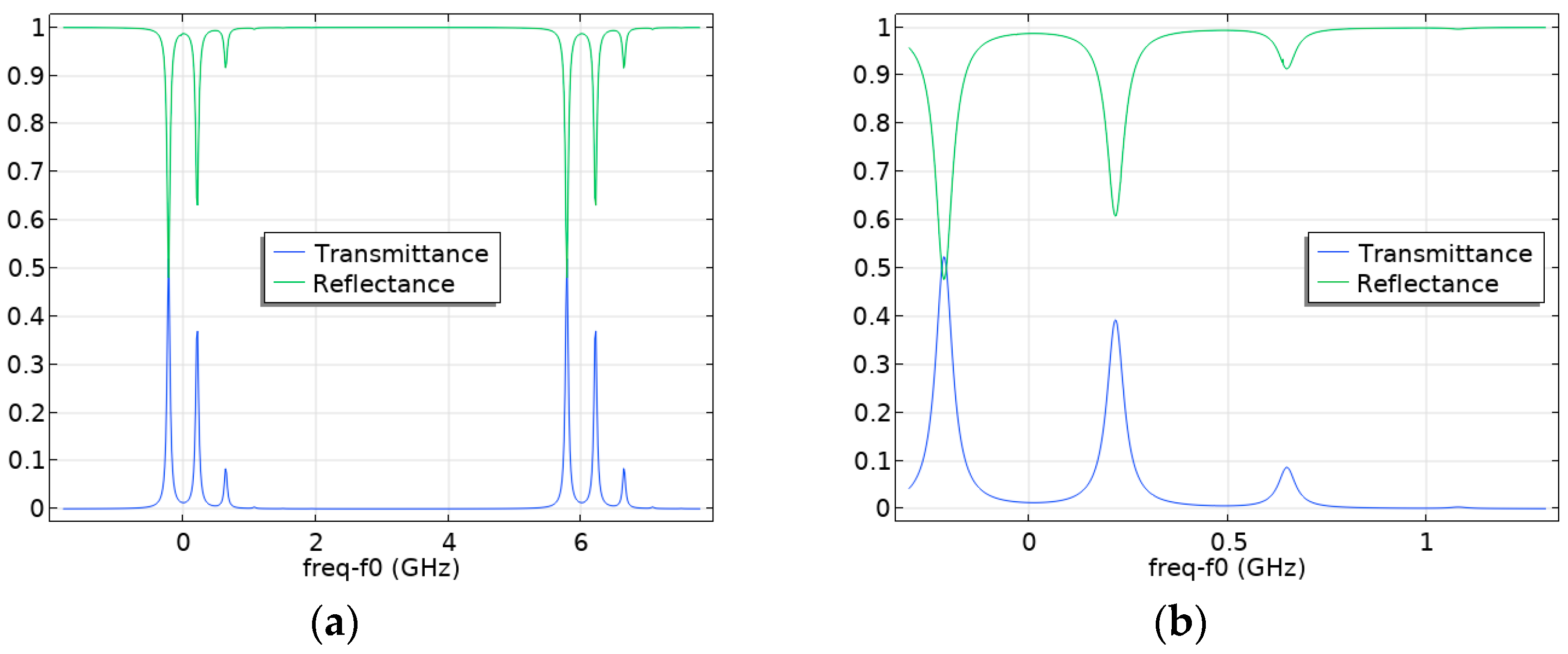
4.1. Investigation of the Influence of the Tilt Angle of a Flat Fabry–Pérot Cavity Mirror on the Appearance of Higher Modes

When using the Fabry–Pérot cavity as a displacement indicator in an optomechanical accelerometer, one of the cavity mirrors is made spherical and concave, and the second mirror is a flat polished front surface of the moving test mass. In this case, an analytical solution to the problem of electromagnetic wave propagation in the Fabry–Pérot cavity is impossible, and numerical methods are required. The geometry and parameters of the system under study were the same as in the previous case (see Section 3), and the only difference was the replacement of the left concave hemisphere with a flat surface (see 4 in Figure 1).

For the system under consideration, the reflectivity of the Fabry–Pérot cavity mirrors R₁ and R₂ were equal to 0.7656. The distance between the mirrors is L_cav = 25 mm, and a laser with a wavelength of λ_L = 1550 nm is used. Then Δν_FSR ≈ 6 GHz, F_c = 116.2.

As the calculations performed have shown, the curve of the resonance sweep for the Fabry–Pérot cavity with the described parameters practically coincides with the case of two spherical mirrors (see Figure 2) except the appearance of a minor second mode with a relative amplitude of A₂ ≈ 0.01·A₁ (where A₁ is the normalized amplitude of the fundamental mode, A₂ is the normalized amplitude of the second mode), while the amplitude of the fundamental mode decreases by the same amount (see Figure 5).

Let us consider the effect of the tilt of the flat mirror of the Fabry–Pérot cavity α on the appearance of higher modes and the resulting decrease in the level of the fundamental mode. As can be seen from the simulation results presented in Figure 6, even a slight tilt angle α = 0.003° causes the occurrence of higher modes. However, their amplitude levels are small—they do not exceed 3% of the level of the fundamental mode.

Increasing the tilt angle to α = 0.01° causes the appearance of higher modes, the amplitude levels of which already make up to 16% of the level of the fundamental mode (see Figure 7).

Increasing the tilt angle to α = 0.012° leads to further amplifying higher modes, the amplitude levels of which already make up to 22% of the level of the fundamental mode (see Figure 8).

When the tilt angle of the flat mirror of the Fabry–Pérot cavity is set to α = 0.014°, the amplitude level of the higher modes is 27% of the fundamental mode level, and a third mode appears, the amplitude of which, however, is small (see Figure 9).

Further increase in α to 0.015° causes the appearance of a more pronounced third mode (A₃ is the normalized amplitude of the third mode) (see Figure 10).

When the tilt angle increases to α = 0.02°, the amplitude of the second mode is 39% of the fundamental mode level, and that of the third mode is 8% (see Figure 11).

Figure 12a shows the dependence of the value of A₁ on the level of α. From the numerical analysis of the influence of the tilt angle of the flat Fabry–Pérot cavity mirror, it follows that additional modes have practically no effect on the fundamental one at a tilt angle of α ≤ 0.003°; in this case, the decrease in the amplitude of the first mode does not exceed 3% (see Figure 6 and Figure 12a). The curve characterizing the degree of dependence of the normalized amplitude of the fundamental mode A₁ on the α level is shown in Figure 12a.

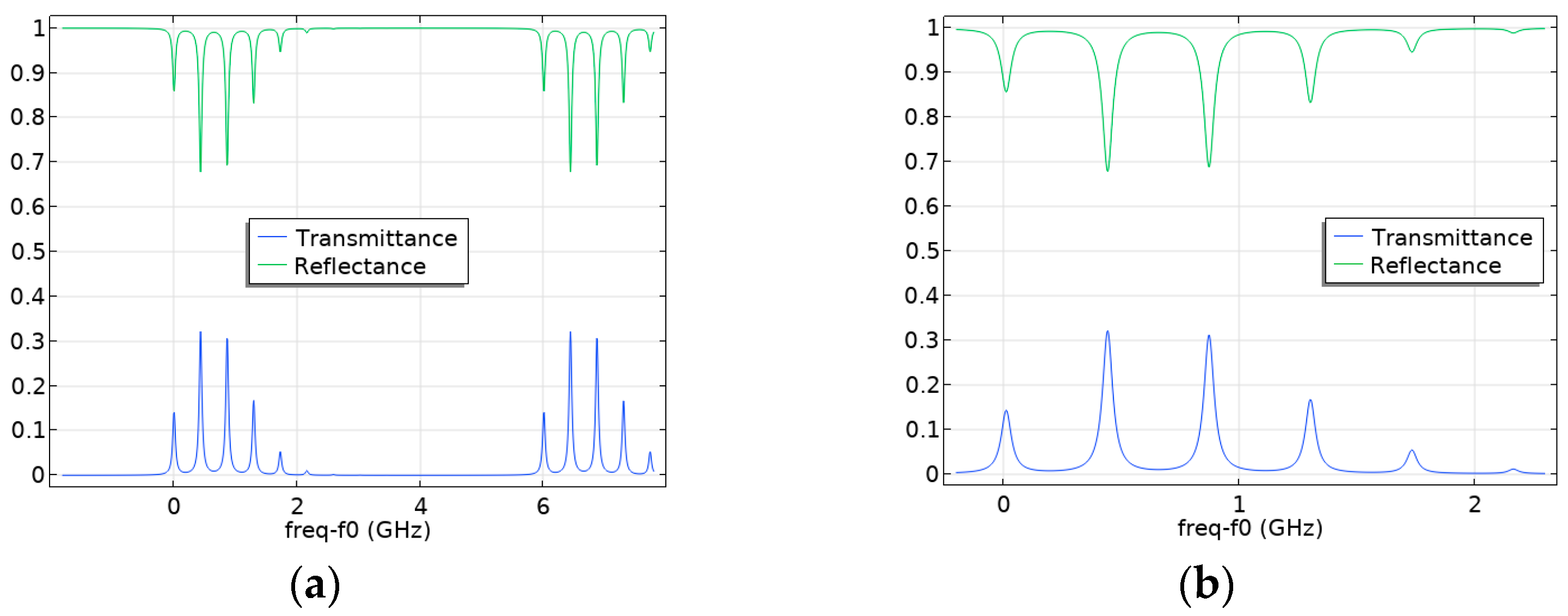
4.2. Investigation of the Influence of the Displacement of the Axis of the Fabry–Pérot Cavity Spherical Mirror on the Occurrence of Higher Modes

Another important parameter influencing the alignment of Fabry–Perot cavities and the appearance of higher modes is the displacement of the axis of the Fabry–Pérot cavity spherical mirror in the vertical direction relative to the laser beam axis that coincides with the cavity axis. Let us denote this displacement as b_R. Since an analytical solution for the “flat mirror—spherical mirror” cavity cannot be obtained, numerical simulation of wave propagation processes was used. Let us first consider a relatively large displacement b_R relative to the cavity height h_cav (see Figure 1). Figure 13 shows the calculated curves of the resonance sweep for the case of b_R = h_cav × 0.05. Figure 13a corresponds to the sweep for the frequency range between two consecutive maxima, and Figure 13b shows the frequency range near the first resonance. As can be seen from Figure 13, such a displacement of the spherical mirror axis relative to the laser beam axis leads to the occurrence of higher modes and beam breakup. In this case, six maxima appear, the amplitude of each of which is reduced by three or more times compared to the case of no displacement of the axes.

When the displacement between the axis of the laser and the cavity decreases: b_R = h_cav × 0.02, the number of maxima decreases to three, and the maximum amplitude of the higher modes does not exceed 27% of the amplitude in the absence of displacement of the axes (see Figure 14).

With a further decrease in the displacement between the axis of the laser and the cavity to b_R = h_cav × 0.01, only two maxima remain, and their maximum amplitude is less than 10% of the amplitude in the case of no displacement of the axes (see Figure 15).

As the modeling showed, the reduction in the displacement value to b_R = h_cav × 0.005 less ensures the alignment of Fabry–Pérot cavities (see Figure 16). In this case, the maximum amplitudes of the higher modes do not exceed 3% of the amplitude in the absence of the axes’ displacement (see Figure 12b and Figure 16). The curve characterizing the degree of dependence of the normalized amplitude of the fundamental mode A₁ on the b_R level is shown in Figure 12b.

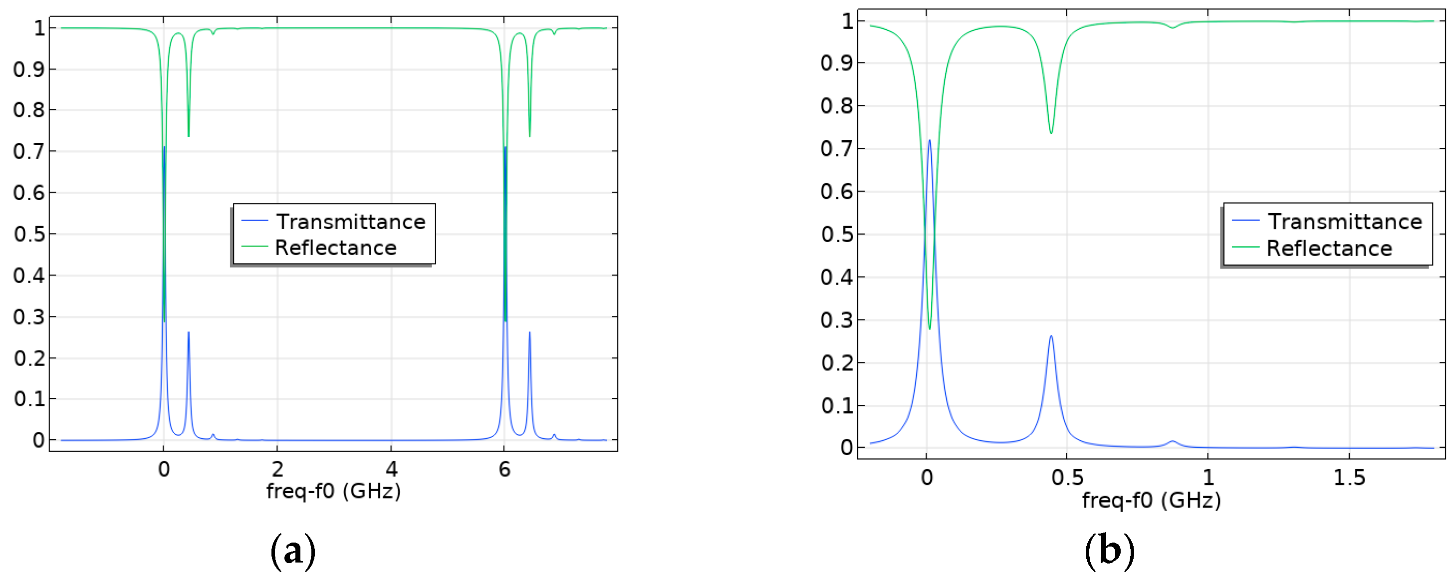
4.3. Investigation of the Influence of the Degree of Laser Beam Axis Displacement on the Occurrence of Higher Modes in the Fabry–Pérot Cavity

Let us consider the influence of the laser beam axis offset relative to the Fabry–Pérot cavity axis on the occurrence of higher modes. The laser beam diameter was set as follows: D_L = 0.5 mm. Figure 17 shows the calculated curves of the resonance sweep for the frequency range in the case of an asymmetrical beam arrangement relative to the Fabry–Pérot cavity axis, namely when the laser beam axis is located at the distance ΔH above the cavity axis. At ΔH = 0.06 × D_L = 0.03 mm, the second mode appears. Still, its amplitude does not exceed 3% of the maximum possible level (see Figure 17c). As shown in Figure 18, the contribution of higher modes increases with an increase in the offset ΔH of the laser beam axis relative to the Fabry–Pérot cavity axis. Thus, at ΔH = 0.125 × D_L = 0.0625 mm, the second mode amplitude is about 9% of the maximum possible (see Figure 18c). A further increase in the laser beam axis displacement to ΔH = 0.25 × D_L = 0.125 mm leads to the appearance of the second mode with a larger amplitude, which is approximately 29% of the maximum amplitude level (see Figure 19) and a third mode with a relatively small level. At ΔH = 0.5 × D_L = 0.25 mm, the beam splits into four modes, the amplitudes of 8% to 40% of the maximum level (see Figure 20).

It follows from the modeling that at the laser beam axis location above the cavity axis at the distance ΔH = 0.06 × D_L = 0.03 mm and less, the alignment of Fabry–Pérot cavities as the maximum amplitudes of the higher modes does not exceed 3% of the amplitude in the absence of the axes’ displacement (see Figure 17; Figure 12c, curve 1).

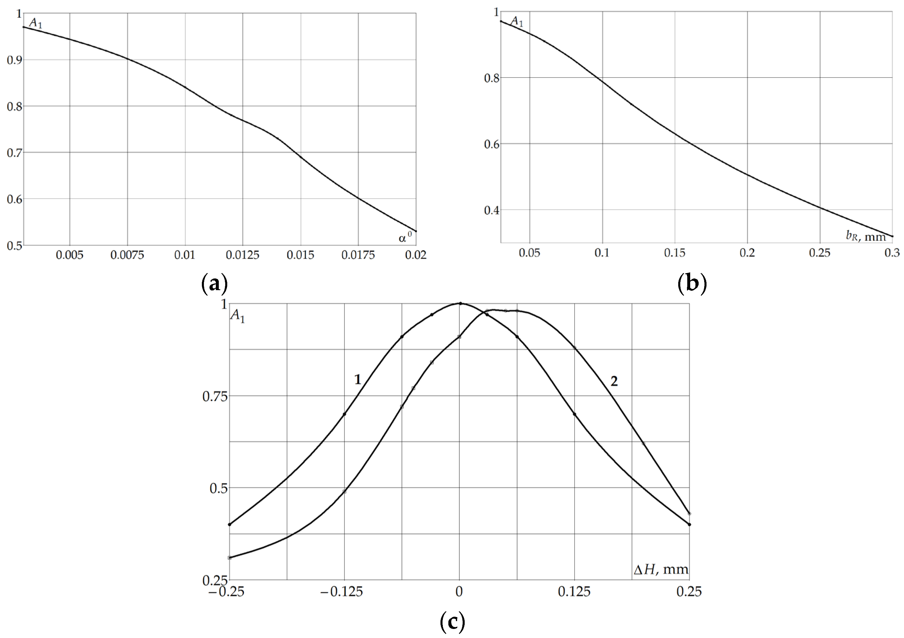
4.4. Investigation of the Influence of the Combinations of Displacements of Various Parameters of the Fabry–Pérot Cavity on the Appearance of Higher Modes

Let us consider the cases when displacements of several different parameters occur simultaneously in the Fabry–Pérot cavity. Let us set the levels of minimum displacements of all three parameters under consideration, each of which individually causes a decrease in the level of the fundamental mode by no more than 3%, namely: α = 0.003°, b_R = h_cav × 0.005 = 0.03 mm, and ΔH = 0.06 × D_L = 0.03 mm. The remaining parameters were the same as described above. As follows from the modeling, the decrease in the amplitude of the fundamental mode in this case does not exceed the permissible levels, namely 3%.

The simulation was also performed when one of the three considered parameters of the Fabry–Pérot cavity has no deviation, and the deviations of the other two are within the values described above as permissible. In this case, if the deviations of the Fabry–Pérot cavity parameters are such that their combination increases the degree of asymmetry of the cavity and the laser beam, the decrease in the fundamental mode level exceeds the permissible levels of 3%. Figure 21 shows the calculated curves of the resonance sweep for the frequency range for one such case when the parameter levels are as follows: α = 0.003°, b_R = 0, ΔH = −0.06 × D_L = −0.03 mm, and the decrease in the fundamental mode level is 8%. The emergence of higher modes is because, with a positive tilt of a flat mirror, the distance between it and a spherical mirror in the area above the cavity axis y = 0 (see Figure 1) increases, and in the area below this axis it decreases; thus, the displacement of the laser beam axis below the cavity axis adds to the rise in the degree of asymmetry, and the decrease in the fundamental mode level increases.

The decrease in the fundamental mode and the appearance of higher modes can also be observed when the tilt angle of the flat mirror is zero, but b_R and ΔH are not. Let us consider a case when the displacements of the axes of the spherical mirror and the laser beam occur in different directions, namely, the mirror axis is shifted upward, and the laser beam axis is shifted downward: α = 0, b_R = h_cav × 0.005 = 0.03 mm, and ΔH = −0.06 × D_L = −0.03 mm. Here, a decrease in the level of the fundamental mode is 9%: A₁ = 0.91, A₂ = 0.085, and A₃ = 0.005 (see Figure 22). The emergence of the higher mode is because the distance between the spherical mirror and the flat mirror in the area above the cavity axis y = 0 (see Figure 1) increases and in the area below the axis y = 0 it decreases, so, the displacement of the laser beam axis below the cavity axis adds to the rise in the degree of asymmetry.

The simulation also showed that if the displacements of the cavity parameters occur in the same direction, for example, for cavities with the following parameters: α = 0, b_R = h_cav × 0.005 = 0.03 mm, ΔH = 0.06 × D_L = 0.03 mm or α = 0.003°, b_R = 0, and ΔH = 0.06 × D_L = 0.03 mm, the decrease in the fundamental mode level does not exceed 3%. Such an effect is due to some compensation of the non-symmetry of the cavities as the greater the degree of asymmetry, the more significant the proportion of higher harmonics, and therefore, the greater the diffraction losses and changes in the shape of the electromagnetic wave [12].

The dependence of A₁ on the level of the laser beam axis shift below the Fabry–Pérot cavity axis in the vertical direction (−ΔH) was also studied in the absence of α and b_R shifts: α = 0, b_R = 0 (see the left part of curve 1 in Figure 12c). The A₁(±ΔH) dependence was also studied in the presence of α and b_R small shifts: α = 0.003°, b_R = h_cav × 0.005 = 0.03 mm (see curve 2 in Figure 12c). As follows from the presented results, when the laser beam axis is shifted up and down relative to the cavity axis, the A₁(ΔH) curve is symmetrical relative to the cavity axis (at ΔH = 0) only in the absence of shifts of α and b_R (see curve 1 in Figure 12c) and it is significantly asymmetrical in the presence of such shifts (see Figure 12c, curve 2).

5. Discussion

Despite the previous studies, including both analytical models [12,18] and experiments [13,14,16] devoted to the Fabry–Pérot cavity misalignment, the determination of the ranges of variation of the main parameters of the “flat mirror—spherical mirror” cavity, within which an acceptable decrease in the fundamental mode amplitude is still ensured, has not been carried out. Analytical models do not allow us to investigate the effect of asymmetry of the parameters of such a Fabry–Pérot cavity, which is used in optomechanical accelerometers; therefore, the numerical studies conducted are relevant. Even if it is qualitatively clear how various parameters affect the asymmetry of a Fabry–Pérot cavity, numerical modeling is effective in obtaining quantitative values. The importance of such studies is determined by the need for preliminary information on the acceptable levels of dimensional deviations during the assembly of the “mechanical resonator—Fabry–Pérot cavity” systems, which are the main part of the optomechanical accelerometer. It is also essential to study the effect of a combination of various parameters affecting the emergence of higher order spatial modes and a decrease in the fundamental mode level. Such investigations also have not been carried out previously. Since the manufacturing mechanical resonators of optomechanical accelerometers and their assembly with the Fabry–Pérot cavity is expensive and time consuming, the planned experimental studies will be carried out further considering the obtained modeling data.

After the assembly of an optomechanical accelerometer and a Fabry–Pérot cavity is manufactured, it must be tested to determine the possible asymmetry of its elements that could cause higher order spatial modes to appear during operation. Experiments that investigate the distributions of the fundamental harmonic mode that occurs in the Fabry–Pérot cavity during scans that involve deviation of the laser beam axis from the cavity axis in the vertical and horizontal directions can be used for such testing. As follows from the modeling of the dependence of the normalized amplitude of the fundamental mode on the deviation of the laser beam axis from the Fabry–Pérot cavity axis in the vertical direction (±ΔH), in the case when the other parameters under consideration (α and b_R) have no deviations, the distribution of A₁(±ΔH) is symmetrical (see Figure 12c, curve 1). If the parameters α and b_R have even minor deviations, for example, those levels, the presence of which does not cause misalignment (α = 0.003°—see Figure 12a, b_R = h_cav × 0.005 = 0.03 mm—see Figure 12b), then the distribution A₁(±ΔH) becomes essentially asymmetrical (see Figure 12c, curve 2). This asymmetry is explained by the fact that when the displacement of the spherical mirror axis (b_R > 0) and/or the angle of inclination of the flat mirror (α > 0) occur in the same direction as the displacement of the laser beam axis (ΔH > 0), some compensation of the asymmetry happens compared to the case when such displacements of b_R and α are absent (b_R = 0, α = 0), and the modulus of the fundamental mode decreases less (compare the right parts of curves 1 and 2 in Figure 12c). If the direction of the laser beam axis displacement does not coincide with the directions of displacements of b_R and α (b_R > 0, α > 0, ΔH < 0), then an increase in the degree of asymmetry in comparison with the case when b_R = 0, α = 0, ΔH < 0 occurs (compare the left parts of curves 1 and 2 in Figure 12c).

As already indicated above, this is explained by the fact that when the parameters are shifted in the same direction, the asymmetry of the system somewhat decreases. When shifted in different directions, the asymmetry of the system increases. This feature can be used to assess whether the asymmetry of the assembly “mechanical resonator—Fabry–Pérot cavity” can cause cavity misalignment. If the dependence A₁(±ΔH) is asymmetrical when the laser beam axis is shifted vertically or horizontally, then the asymmetry of the assembly will cause cavity misalignment. Despite the seeming obviousness of this approach, the main thing in its application is the quantitative differences between the amplitude levels of the fundamental mode when the laser beam axis moves above or below the resonator axis. As shown in Figure 12c, the asymmetry of the curve A₁(±ΔH) is quite significant, even with minor deviations in the cavity parameter values.

6. Conclusions

A model for describing the processes of wave optics during the passage of a laser beam through a Fabry–Pérot cavity is implemented numerically using the finite element method in the COMSOL Multiphysics package. The case when two spherical mirrors form the Fabry–Pérot cavity is considered; a comparison of the results obtained using this model with the results of the analytical solution [12] is carried out, which showed their coincidence within 2–3%. Numerical modeling revealed that in a Fabry–Pérot cavity consisting of a flat and a spherical mirror, when the laser beam axis is shifted vertically relative to the cavity axis, the wave splits into two higher modes or more, which coincides with the experimental data for such a case [16].

Using the performed numerical simulation, we obtained dependences characterizing the decrease in the fundamental mode amplitude for various values of the deviations of the system parameters from the symmetrical arrangement. Thus, the displacement of the spherical mirror axis in the vertical direction relative to the laser beam axis, coinciding with the cavity axis, by a value no greater than 0.5% of the cavity height leads to a decrease in the fundamental mode amplitude by no more than 3% (see Figure 12b and Figure 16). Inclination of the flat Fabry–Pérot cavity mirror by angles less than 0.003° leads to a decrease in the fundamental mode amplitude by no more than 3% (see Figure 6 and Figure 12a). The displacement of the laser beam axis does not lead to a decrease in the fundamental mode amplitude by more than 3% if the value of this displacement does not exceed 6% of the laser beam diameter (see Figure 17; Figure 12c, curve 1).

As can be seen from the calculated curves of the reduction in the fundamental mode levels depending on the tilt angle of a flat Fabry–Pérot cavity mirror α—Figure 12a, the displacement of the axis of the Fabry–Pérot cavity spherical mirror b_R—Figure 12b, the degree of laser beam axis displacement ΔH—Figure 12c, the most significant influence on the misalignment of the Fabry–Pérot cavity causes the level of tilt angle of a flat Fabry–Pérot cavity mirror. The dependences of the fundamental mode levels on the values of b_R and ΔH are similar since they belong to the same type of asymmetry. Thus, when assembling a mechanical resonator and a Fabry–Pérot cavity “flat mirror—spherical mirror”, primary attention should be paid to monitoring the parallelism of its flat mirror.

The combination of displacements of different parameters of the Fabry–Pérot cavity can cause either a decrease or an increase in the degree of the cavity misalignment (see Figure 12c, curve 2). This property can be used to evaluate the quality of the Fabry–Pérot cavity assembly with the mechanical resonator, as suggested in the Discussion section.

References

1. Costa, G.K.B.; Gouvêa, P.M.P.; Soares, L.M.B.; Pereira, J.M.B.; Favero, F.; Braga, A.M.; Palffy-Muhoray, P.; Bruno, A.C.; Carvalho, I.C. In–fiber Fabry–Perot interferometer for strain and magnetic field sensing. Opt. Express 2016, 24, 14690–14696. [Google Scholar] [CrossRef]
2. Frazão, O.; Aref, S.H.; Baptista, J.M.; Santos, J.L.; Latifi, H.; Farahi, F.; Kobelke, J.; Schuster, K. Fabry–Pérot Cavity Based on a Suspended–Core Fiber for Strain and Temperature Measurement. IEEE Photon. Technol. Lett. 2019, 21, 1229–1231. [Google Scholar] [CrossRef]
3. Ferreira, M.S.; Coelho, L.; Schuster, K.; Kobelke, J.; Santos, J.L.; Frazão, O. Fabry–Perot cavity based on a diaphragm–free hollow–core silica tube. Opt. Lett. 2011, 36, 4029. [Google Scholar] [CrossRef] [PubMed]
4. Ferreira, M.S.; Bierlich, J.; Kobelke, J.; Schuster, K.; Santos, J.L.; Frazao, O. Towards the control of highly sensitive Fabry–Perot strain sensor based on hollow–core ring photonic crystal fiber. Opt. Express 2012, 20, 21946. [Google Scholar] [CrossRef]
5. Liu, S.; Yang, K.; Wang, Y.; Qu, J.; Liao, C.; He, J.; Li, Z.; Yin, G.; Sun, B.; Zhou, J.; et al. High–sensitivity strain sensor based on in–fiber rectangular air bubble. Sci. Rep. 2015, 5, 7624. [Google Scholar] [CrossRef] [PubMed]
6. Islam, M.R.; Ali, M.M.; Lai, M.-H.; Lim, K.-S.; Ahmad, H. Chronology of Fabry–Perot Interferometer Fiber–Optic Sensors and Their Applications: A Review. Sensors 2014, 14, 7451–7488. [Google Scholar] [CrossRef] [PubMed]
7. Guzmán, C.F.; Kumanchik, L.; Pratt, J.; Taylor, J.M. High sensitivity optomechanical reference accelerometer over 10 kHz. Appl. Phys. Lett. 2014, 104, 221111. [Google Scholar] [CrossRef]
8. Li, B.; Ou, L.; Lei, Y.; Liu, Y. Cavity optomechanical sensing. Nanophotonics 2021, 10, 2799–2832. [Google Scholar] [CrossRef]
9. Reschovsky, B.J.; Long, D.A.; Zhou, F.; Bao, Y.; Allen, R.A.; LeBrun, T.W.; Gorman, J.J. Intrinsically accurate sensing with an optomechanical accelerometer. Opt. Express 2022, 30, 19510–19523. [Google Scholar] [CrossRef]
10. Hines, A.; Nelson, A.; Zhang, Y.; Valdes, G.; Sanjuan, J.; Stoddart, J.; Guzmán, F. Optomechanical Accelerometers for Geodesy. Remote Sens. 2022, 14, 4389. [Google Scholar] [CrossRef]
11. Ismail, N.; Kores, C.C.; Geskus, D.; Pollnau, M. Fabry–Pérot resonator: Spectral line shapes, generic and related Airy distributions, linewidths, finesses, and performance at low or frequency–dependent reflectivity. Opt. Express 2016, 24, 16366–16389. [Google Scholar] [CrossRef] [PubMed]
12. Anderson, D.Z. Alignment of resonant optical cavities. Appl. Opt. 1984, 23, 2944–2949. [Google Scholar] [CrossRef] [PubMed]
13. Takamori, A.; Araya, A.; Morii, W.; Telada, S.; Uchiyama, T.; Ohashi, M. A 100-m Fabry–Pérot Cavity with Automatic Alignment Controls for Long-Term Observations of Earth’s Strain. Technologies 2014, 2, 129–142. [Google Scholar] [CrossRef]
14. Wang, W.; Zhou, C.; Zhang, T.; Chen, J.; Liu, S.; Fan, X. Optofluidic laser array based on stable high-Q Fabry–Pérot microcavities. Lab A Chip 2015, 15, 3862–3869. [Google Scholar] [CrossRef] [PubMed]
15. Gerberding, O.; Guzmán, C.F.; Melcher, J.; Pratt, J.R.; Taylor, J.M. Optomechanical reference accelerometer. Metrologia 2015, 52, 654–665. [Google Scholar] [CrossRef]
16. Durand, M.; Wang, Y.; Lawall, J. Accurate Gouy phase measurement in an astigmatic optical cavity. Appl. Phys. B 2012, 108, 749–753. [Google Scholar] [CrossRef]
17. The Feynman Lectures on Physics. Available online: https://mathphyche.wordpress.com/wp-content/uploads/2020/01/the-feynman-lectures-on-physics-vol.-ii_-the-new-millennium-edition_-mainly-electromagnetism-and-matter.pdf (accessed on 10 October 2024).
18. Kogelnik, H.; Li, T. Laser Beams and Resonators. Appl. Opt. 1966, 5, 1550–1567. [Google Scholar] [CrossRef] [PubMed]
19. Rezinkina, M.; Braxmaier, C. Designs of Miniature Optomechanical Sensors for Measurements of Acceleration with Frequencies of Hundreds of Hertz. Designs 2024, 8, 67. [Google Scholar] [CrossRef]
20. Available online: https://doc.comsol.com/5.6/doc/com.comsol.help.models.woptics.fabry_perot_resonator/fabry_perot_resonator.html (accessed on 10 October 2024).
21. Available online: https://doc.comsol.com/5.4/doc/com.comsol.help.woptics/WaveOpticsModuleUsersGuide.pdf (accessed on 10 October 2024).
Figure 1. Computational domain with grid. y = 0 corresponds to the cavity axis of symmetry.
Photonics 12 00015 g001
Figure 2. Calculated curves of the resonance sweep for the frequency range, including the two main resonant frequencies (a) and near the first resonance (b).
Photonics 12 00015 g002
Figure 3. Calculated curves of the resonance sweep for the frequency range, including the two main resonant frequencies (a) and near the first resonance (b) at the vertical displacement level ay/w0 = 0.15.
Photonics 12 00015 g003
Figure 4. Calculated curves of the resonance sweep for the frequency range, including the two main resonant frequencies (a) and near the first resonance (b) at the displacement level ay/w0 = 0.3.
Photonics 12 00015 g004
Figure 5. Calculated curves of the resonance sweep for the frequency range, including the two main resonant frequencies (a) and near the first resonance (b) for the case of one flat and one curved mirror of the Fabry–Pérot cavity. A1 = 0.99, A2 = 0.01.
Photonics 12 00015 g005
Figure 6. Calculated curves of the resonance sweep for the frequency range, including the two main resonant frequencies (a) and near the first resonance (b) at the level of the plane mirror tilt α = 0.003°. A1 = 0.97, A2 = 0.02, and A3 = 0.01.
Photonics 12 00015 g006
Figure 7. Calculated curves of the resonance sweep for the frequency range, including the two main resonant frequencies (a) and near the first resonance (b) at the level of the plane mirror tilt α = 0.01°. A1 = 0.84, A2 = 0.16.
Photonics 12 00015 g007
Figure 8. Calculated curves of the resonance sweep for the frequency range, including the two main resonant frequencies (a) and near the first resonance (b) at the level of the plane mirror tilt α = 0.012°. A1 = 0.78, A2 = 0.22.
Photonics 12 00015 g008
Figure 9. Calculated curves of the resonance sweep for the frequency range, including the two main resonant frequencies (a) and near the first resonance (b) at the level of the plane mirror tilt α = 0.014°. A1 = 0.73, A2 = 0.27.
Photonics 12 00015 g009
Figure 10. Calculated curves of the resonance sweep for the frequency range, including the two main resonant frequencies (a) and near the first resonance (b) at the level of the plane mirror tilt α = 0.015°. A1 = 0.69, A2 = 0.295, and A3 = 0.015.
Photonics 12 00015 g010
Figure 11. Calculated curves of the resonance sweep for the frequency range, including the two main resonant frequencies (a) and near the first resonance (b) at the level of the plane mirror tilt α = 0.02°. A1 = 0.53, A2 = 0.39, and A3 = 0.08.
Photonics 12 00015 g011
Figure 12. Calculated dependencies of the normalized amplitude of the fundamental mode A1: (a)—A1 (α); (b)—A1 (bR); and (c)—A1H) (where curve 1 corresponds to the case of absence of displacements of α and bR; curve 2 corresponds to the case of the levels of displacements of α and bR: α = 0.003°, bR = hcav × 0.005 = 0.03 mm). A high-frequency mode with the normalized amplitude A2 = 1 − A1 appears at 0.5 < A1 ≤ 0.97; at A1 < 0.5, the wave splits into three or more modes.
Photonics 12 00015 g012
Figure 13. Calculated curves of the resonance sweep for the frequency range, including the two main resonant frequencies (a) and near the first resonance (b) for the level of the spherical Fabry–Pérot cavity mirror axis displacement in the vertical direction bR = hcav × 0.05 = 0.3 mm. A0 = 0.15, A1 = 0.32, A2 = 0.3, A3 = 0.17, A4 = 0.05, and A5 = 0.01 (where An is the normalized amplitude of the n–mode).
Photonics 12 00015 g013
Figure 14. Calculated curves of the resonance sweep for the frequency range, including the two main resonant frequencies (a) and near the first resonance (b) for the level of the spherical Fabry–Pérot cavity mirror axis displacement in the vertical direction bR = hcav × 0.02 = 0.12 mm. A1 = 0.72, A2 = 0.27, and A3 = 0.01.
Photonics 12 00015 g014
Figure 15. Calculated curves of the resonance sweep for the frequency range, including the two main resonant frequencies (a) and near the first resonance (b) for the level of the spherical Fabry–Pérot cavity mirror axis displacement in the vertical direction bR = hcav × 0.01 = 0.06 mm. A1 = 0.91, A2 = 0.09.
Photonics 12 00015 g015
Figure 16. Calculated curves of the resonance sweep for the frequency range, including the two main resonant frequencies (a) and near the first resonance (b) for the level of the spherical Fabry–Pérot cavity mirror axis displacement in the vertical direction bR = hcav × 0.005 = 0.03 mm. A1 = 0.97, A2 = 0.018, and A3 = 0.012.
Photonics 12 00015 g016
Figure 17. Calculated curves of the resonance sweep for the frequency range, including the two main resonant frequencies (a) and near the first resonance (b), (c) for the level of the offset of the laser beam axis ΔH = 0.06 × DL = 0.03 mm. A1 = 0.97, A2 = 0.03.
Photonics 12 00015 g017
Figure 18. Calculated curves of the resonance sweep for the frequency range, including the two main resonant frequencies (a) and near the first resonance (b), (c) for the level of the offset of the laser beam axis ΔH = 0.125 × DL = 0.0625 mm. A1 = 0.91, A2 = 0.09.
Photonics 12 00015 g018
Figure 19. Calculated curves of the resonance sweep for the frequency range, including the two main resonant frequencies (a) and near the first resonance (b), (c) for the level of the offset of the laser beam axis ΔH = 0.25 × DL = 0.125 mm. A1 = 0.70, A2 = 0.29, and A3 = 0.01.
Photonics 12 00015 g019
Figure 20. Calculated curves of the resonance sweep for the frequency range, including the two main resonant frequencies (a) and near the first resonance (b), (c) for the level of the offset of the laser beam axis ΔH = 0.5 × DL = 0.25 mm. A1 = 0.40, A2 = 0.26, and A3 = 0.08.
Photonics 12 00015 g020
Figure 21. Calculated curves of the resonance sweep for the frequency range, including the two main resonant frequencies (a) and near the first resonance (b) for the levels of the offsets α = 0.003°, bR = 0, ΔH = −0.06 × DL = −0.03 mm. A1 = 0.92, A2 = 0.075, and A3 = 0.005.
Photonics 12 00015 g021
Figure 22. Calculated curves of the resonance sweep for the frequency range, including the two main resonant frequencies (a) and near the first resonance (b) for the levels of the offsets α = 0, bR = hcav × 0.005 = 0.03 mm, and ΔH = −0.06 × DL = −0.03 mm. A1 = 0.91, A2 = 0.085, and A3 = 0.005.
Photonics 12 00015 g022
Disclaimer/Publisher’s Note: The statements, opinions and data contained in all publications are solely those of the individual author(s) and contributor(s) and not of MDPI and/or the editor(s). MDPI and/or the editor(s) disclaim responsibility for any injury to people or property resulting from any ideas, methods, instructions or products referred to in the content.