Angular Circle Array Multiple Input Multiple Output Underwater Optical Wireless Communications ^†

Abstract

This paper constructs a simulation platform for underwater wireless optical single-input single-output (SISO) communication systems and quantitatively evaluates communication performance indicators. To improve channel capacity, we propose an angular circle array MIMO scheme. The path loss, CIR, and channel capacity of the angular circular array MIMO communication system are calculated by using the Monte Carlo method. Results show that the proposed angular circular array MIMO communication system has a higher channel capacity compared to planar circular array MIMO communication systems and SISO communication systems.

1. Introduction

Underwater wireless communication (UWC) refers to the transmission of data through wireless carriers in an underwater environment, primarily including underwater acoustic communication, underwater radio frequency (RF) communication, and underwater wireless optical communication (UWOC). Although underwater acoustic communication is commonly used for wireless links [1], it has limitations such as low data transmission rates, high latency, and high energy consumption [2]. Additionally, RF communication suffers from high attenuation, which increases dramatically with frequency [3]. Considering the need for high-speed transmission, UWOC technology is a feasible alternative. UWOC not only uses an ultra-wide range of unregulated spectrum to overcome spectrum crisis but also offers advantages like high confidentiality, small footprint, and low latency [4].

Early UWOC modeling studies focused on single-input single-output (SISO) communication systems in case of line-of-sight (LOS) links. Hanson et al. [5] demonstrated 1 Gbps underwater laser communication over a 2 m path in a laboratory environment. Since then, UWOC has become an emerging topic, and researchers have explored higher data rates and longer transmission distances. Wang et al. [6] successfully achieved a data rate of 500 Mbps through a 100 m tap-water channel by using a green laser diode (LD) and non-return-to-zero on-off keying (NRZ-OOK) modulation. Hu et al. [7] demonstrated a 20.09 Gbps transmission over a 1.2 m underwater link with PS bit-loading DMT modulation. Additionally, Fei et al. [8] pushed the transmission distance and data rate to 100.6 m and 3 Gbps, respectively, using a wideband photomultiplier tube. Recently, our group proposed a MIMO scheme, which increased the channel capacity [9].

In fact, UWOC terminals are mostly carried on mobile platforms with low load capacity, such as autonomous underwater vehicles (AUVs) and frogmen. The swaying of these platforms with the currents is inevitable, making the establishment and maintenance of the UWOC link challenging. Additionally, ocean optical applications, such as undersea monitors and tsunami warning systems, require extensive coverage areas for the UWOC systems [10]. To address these issues, one approach is to increase the beam divergence angle and receiver field of view (FOV). However, this leads to more severe absorption and scattering introduced by underwater channels, increasing link loss and time dispersion, thus shortening the communication distance and reducing the channel capacity of the communication systems, especially in turbid water. Traditional wireless communication often uses higher-order modulation to address limited channel capacity, but this method of trading power for bandwidth is not practical in underwater environments with high attenuation. Multiplexing techniques play a vital role in increasing the channel capacity by utilizing spatial freedom resources to combine multiple low-speed data streams into one high-speed stream. Therefore, several researchers have further investigated UWOC using MIMO techniques. Ramavath et al. [11] studied the performance of a UWOC system using on–off keying modulation at a data rate of 500 Mbps over a link range of 30 m. The system uses a transmit/receive diversity scheme, and the closed-form analytical bit error rate (BER) expressions of single-input single-output (SISO), single-input multiple-output (SIMO), MISO, and MIMO links for un-coded and RS-coded cases have been computed using the hyperbolic tangent distribution and validated with Monte Carlo simulation results. Their results show that the MIMO technique effectively reduces the BER of UWOC systems. Muhsin et al. [12] obtained the outage probability expression for a UWOC MIMO communication system in analytical form using the Meijer-G function. In addition to diversity techniques, researchers have also investigated multiplexing techniques for MIMO communication systems. Dong et al. [13] developed a 2 × 2 UWOC MIMO channel model. The simulation results showed that the MIMO channel capacity decreases as the symbol baud rate increases and can be enhanced by increasing the average transmit power or adjusting detector FOV.

Compared to SISO communication systems, MIMO communication systems extend the communication range and increase the channel capacity of systems [14]. Although the commonly used planar MIMO scheme raises the upper limit of the transmission rate to some extent, it requires maintaining strictly aligned links, similar to SISO communication systems. Therefore, developing a novel transceiver architecture for underwater wireless optical MIMO communication systems is crucial.

In this paper, based on the common planar circular array MIMO communication systems, we propose a transceiver architecture design that effectively mitigates communication outages due to link misalignment. It can be assumed that within a certain range of transceiver jitter, each transmitter will always be approximately aligned with a single receiver, thereby achieving a larger communication coverage area.

2. System Model

Three structures of underwater wireless optical communication systems are given in Figure 1. As shown in (a), the transceiver of the SISIO system is fully aligned. As shown in (b), the transceivers of the corresponding numbers of the planar circle array communication system are aligned. We propose an underwater wireless optical angular circle array MIMO communication system based on spatial diversity, which is shown in Figure 1c. All transceivers, except the center transceiver, face outward at an angle. If not otherwise specified, r and t are the receiver and transmitter, respectively. The numbers 1 to 7 are the transceiver labels. Considering the compactness requirements of underwater communication devices, we designed the transceivers with a hemispherical configuration. However, the transmitter array can only approximate a hemispherical shape due to light fluctuation constraining the size of the beam diffusion angle. This design improves the coverage of the wireless communication system so that full mobility can be supported. Notably, this design does not require physically placing the transceivers on a hemispherical structure. Instead, it uses the geometry of the hemisphere to determine the normal vectors of the transceiver planes. The transceiver array structure is then realized by rotating the transceiver planes so that the normal vectors point in different directions.

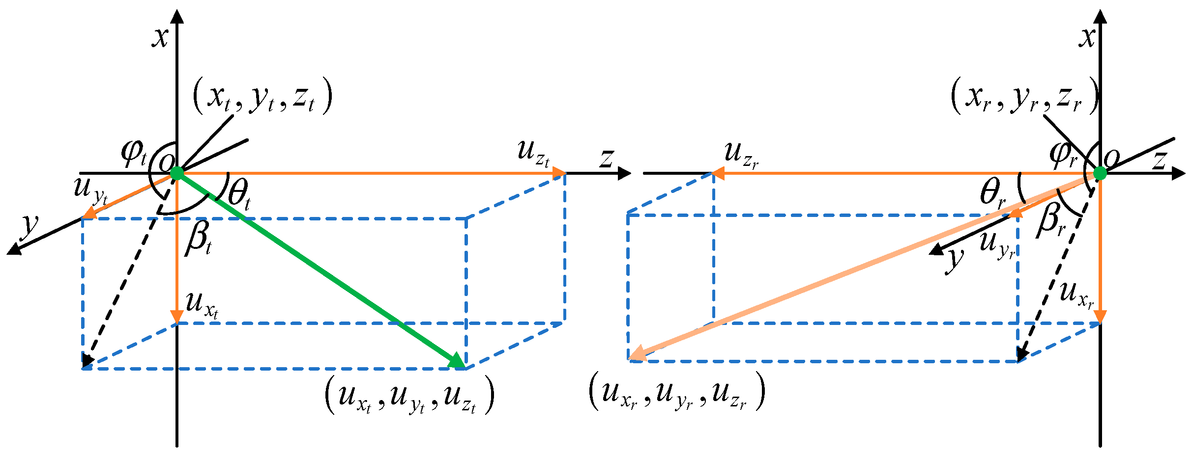
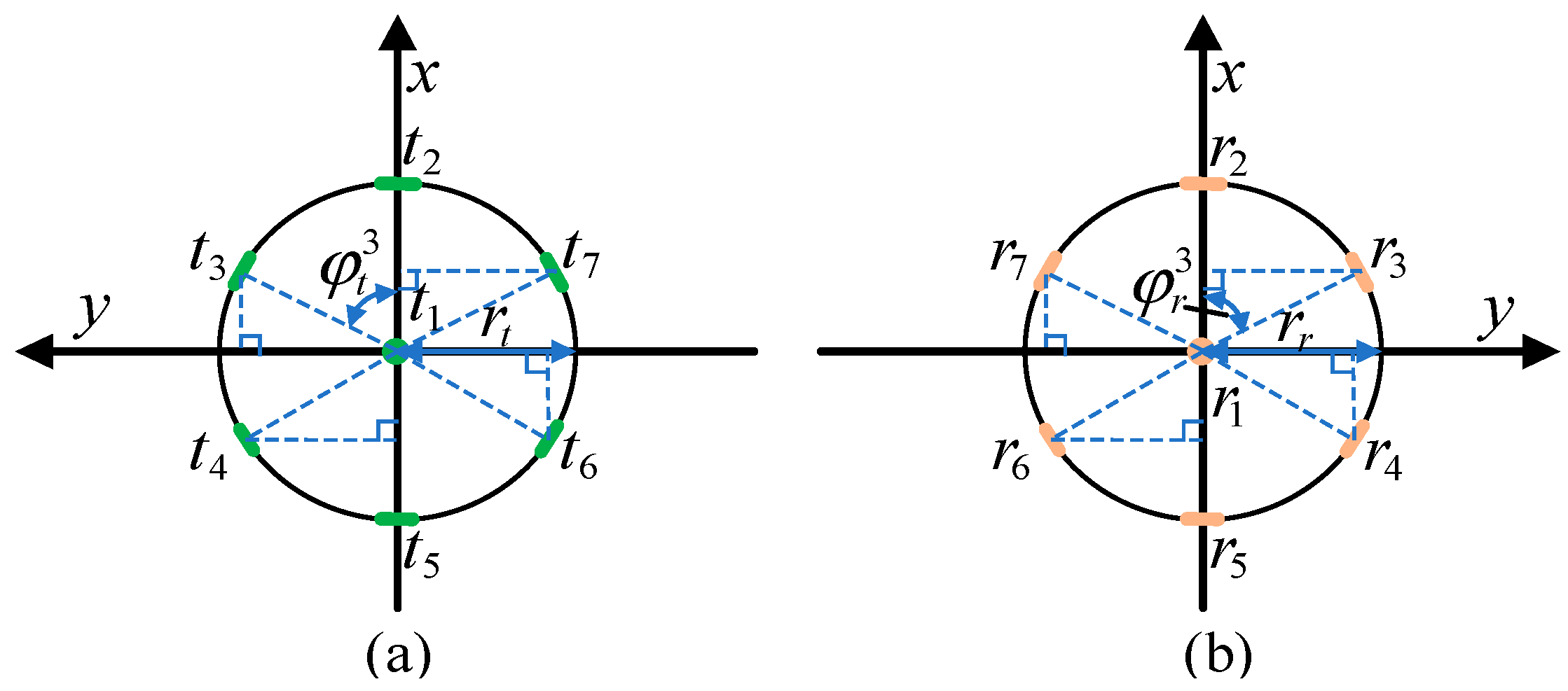
2.1. Definition of Transceiver Parameters

To better match practical application scenarios and facilitate the formula derivation for designing the angular circle array MIMO transceiver structure, we define the transceiver parameters, which are shown in Figure 2. $\theta$, $\beta$, and $\phi$ are the scattering angle, elevation angle, and azimuth angle of the transceiver plane normal vector, respectively. $(u_x,u_y,u_z)$ is the direction cosine of the normal vector of the transceiver plane. $(x,y,z)$ is the coordinate of the transceiver center position.

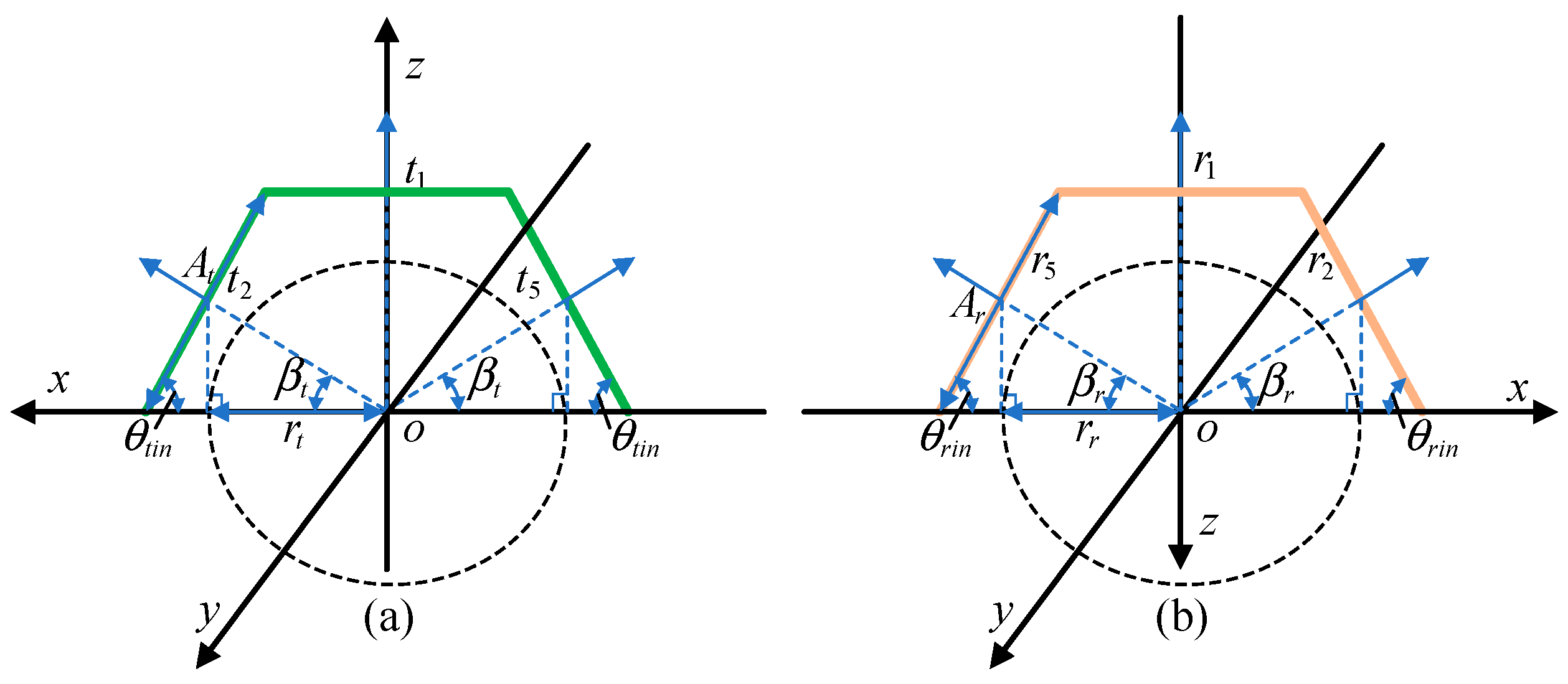
2.2. Transmitter Rotation

Taking one of the transmitters as an example, in the xyz coordinate system, if the transmitter plane is rotated by ${\theta }_t$ and ${\phi }_t$, it is equivalent to the transmitter being rotated by ${\theta }_t$ around the x-axis first and then by ${\phi }_t$ around the z-axis. At this point, the initial coordinates of the photon can be expressed as follows [15]:

$$\left[\begin{array}{c}{x}_0^{\prime }\\ y_0^{\prime }\\ z_0^{\prime }\end{array}\right]=\left[\begin{array}{ccc}1& 0& 0\\ 0& \cos {\theta }_t& \sin {\theta }_t\\ 0& -\sin {\theta }_t& \cos {\theta }_t\end{array}\right]\left[\begin{array}{ccc}\cos {\phi }_t& \sin {\phi }_t& 0\\ -\sin {\phi }_t& \cos {\phi }_t& 0\\ 0& 0& 1\end{array}\right]\left[\begin{array}{c}{x}_0\\ y_0\\ z_0\end{array}\right]·$$

(1)

If the transmitter is displaced, the new initial coordinates of the photon need to be updated as follows: $(x_0^{\prime \prime },y_0^{\prime \prime },z_0^{\prime \prime })=(x_0+x_t,y_0+y_t+z_0+z_t),$ where $(x_t,y_t,z_t)$ is the displacement vector. Due to the angle of rotation of the transmitter, the initial direction cosines of the photon are updated as follows:

$$\left[\begin{array}{c}{u}_{x_0}^{\prime }\\ u_{y_0}^{\prime }\\ u_{z_0}^{\prime }\end{array}\right]=\left[\begin{array}{ccc}1& 0& 0\\ 0& \cos {\theta }_t& \sin {\theta }_t\\ 0& -\sin {\theta }_t& \cos {\theta }_t\end{array}\right]\left[\begin{array}{ccc}\cos {\phi }_t& \sin {\phi }_t& 0\\ -\sin {\phi }_t& \cos {\phi }_t& 0\\ 0& 0& 1\end{array}\right]\left[\begin{array}{c}{u}_{x_0}\\ u_{y_0}\\ u_{z_0}\end{array}\right]·$$

(2)

2.3. Receiver Rotation

Similar considerations are made for the receivers by the scattering angle ${\theta }_r$ and the azimuthal angle ${\phi }_r$. The receiver plane is shown in Figure 3. The plane can be expressed as follows: $Ax+By+Cz+D=0,$ where $A=\sin {\theta }_r\cos {\phi }_r,$ $B=\sin {\theta }_r\sin {\phi }_r,$ $C=\cos {\theta }_r,$ and $D=-A{x}_r-B{y}_r-C{z}_r,$ and ${\overrightarrow{n}}_{vec}=\left(A,B,C\right)$ is the normal vector of the plane.

From Figure 3, we assume that a photon is scattered n − 1 times, and after the nth scattering event due to collision, the photon passes through the receiving plane. In this optical event, the position of the photon before the scattering has the coordinates of point M $\left(x_{n-1},y_{n-1},z_{n-1}\right)$, and the coordinates of the photon after the scattering event are at point N $\left(x_n,y_n,z_n\right)$. The photon coordinates before the nth scattering are above the receiving plane, and the photon coordinates after the nth scattering are below the receiving plane, expressed as follows: $A{x}_{n-1}+B{y}_{n-1}+C{z}_{n-1}+D\ge 0,$ $A{x}_n+B{y}_n+C{z}_n+D\le 0.$ Photons within the receiver plane that pass through the reception plane will be intercepted at the reception plane, and their final path length $s_n$ can be expressed as follows: $s_n=equ\cdot s_{r_n},$ where

$$equ={\displaystyle \frac{A{x}_{n-1}+B{y}_{n-1}+C{z}_{n-1}+D}{\left|A{x}_{n-1}+B{y}_{n-1}+C{z}_{n-1}+D\right|+\left|A{x}_n+B{y}_n+C{z}_n+D\right|}},$$

(3)

and $s_{r_n}$ is the path length traveled by the photon that underwent the last scattering.

According to the above derivation, the actual coordinates of the photon arriving at the receiving plane can be written as follows:

$$\left(x_t,y_t,z_t\right)=\left[\left(x_n,y_n,y_n\right)-\left(x_{n-1},y_{n-1},z_{n-1}\right)\right]\cdot equ+\left(x_n,y_n,y_n\right),$$

(4)

and ${\alpha }_r$ between the direction vector of a photon arriving at the receiving plane and the receiver normal vector can be expressed as follows: ${\alpha }_r=\arccos \left(({\overrightarrow{n}}_{vec}\cdot \overrightarrow{MN})/(\left|{\overrightarrow{n}}_{vec}\right|\left|\overrightarrow{MN}\right|)\right),$ where $\overrightarrow{MN}=\left(x_n-x_{n-1},y_n-y_{n-1},z_n-z_{n-1}\right),$ $\left|{\overrightarrow{n}}_{vec}\right|=\sqrt{A^2+B^2+C^2},$ $\left|\overline{MN}\right|=s_{r_n}.$ Then, ${\alpha }_r$ can also be written as follows:

$${\alpha }_r=\arccos \left({\displaystyle \frac{A\left(x_n-x_{n-1}\right)+B\left(y_n-y_{n-1}\right)+C\left(z_n-z_{n-1}\right)}{\sqrt{A^2+B^2+C^2}{s}_{r_n}}}\right)·$$

(5)

As the receiver plane rotates, the conditions for determining whether a photon is successfully received need to be adjusted. The receiver is defined by three key parameters: the coordinates of the receiver center position $(x_r,y_r,z_r)$, the receiver plane diameter $A_r$, and FOV. Initially, $x_r$ and $y_r$ are both 0, and $z_r$ is the communication distance. As the receiver rotates, photons that satisfy [16]: $\pi -{\alpha }_r\le \mathrm{FOV}/2,$ and

$$A_r\ge \sqrt{{\left(x_{n_r}-x_r\right)}^2+{\left(y_{n_r}-y_r\right)}^2+{\left(z_{n_r}-z_r\right)}^2},$$

(6)

are considered to be received. $(x_{n_r},y_{n_r},z_{n_r})$ is the coordinates of the photon projected onto the receiver plane.

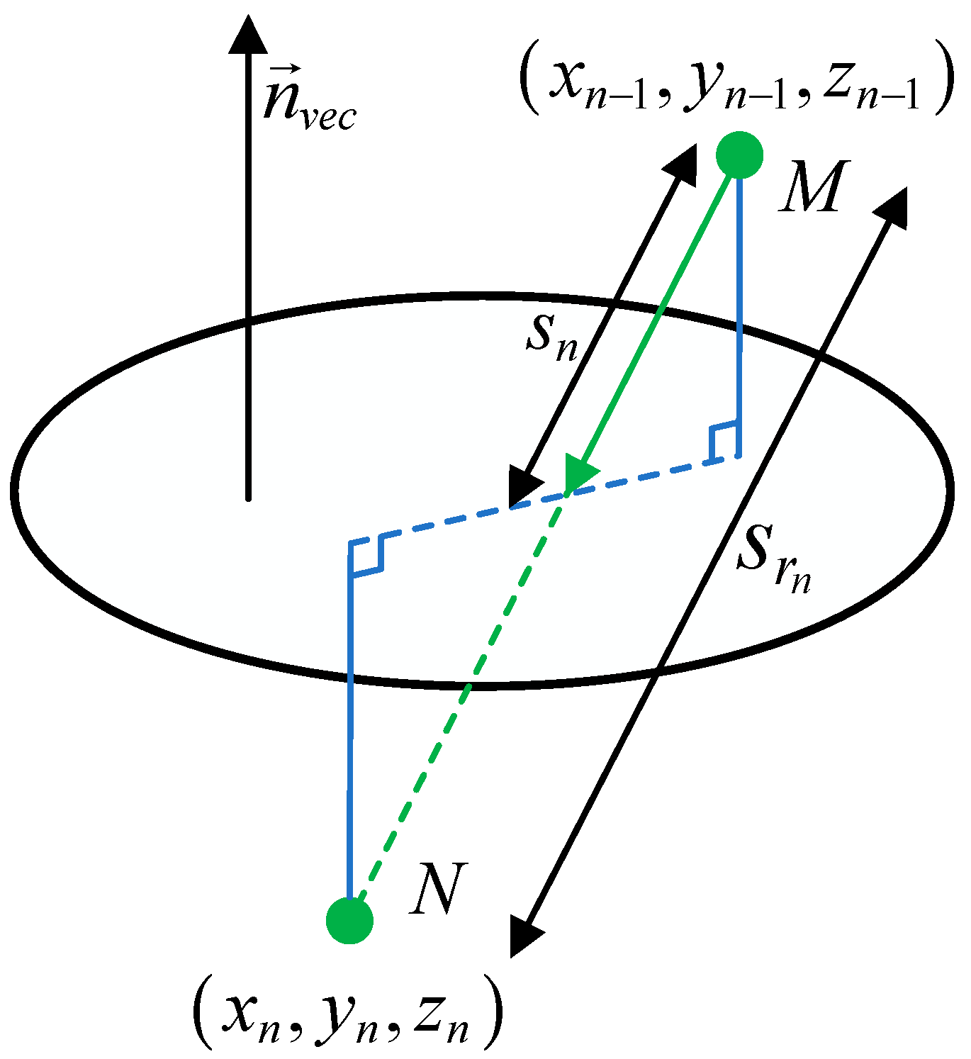
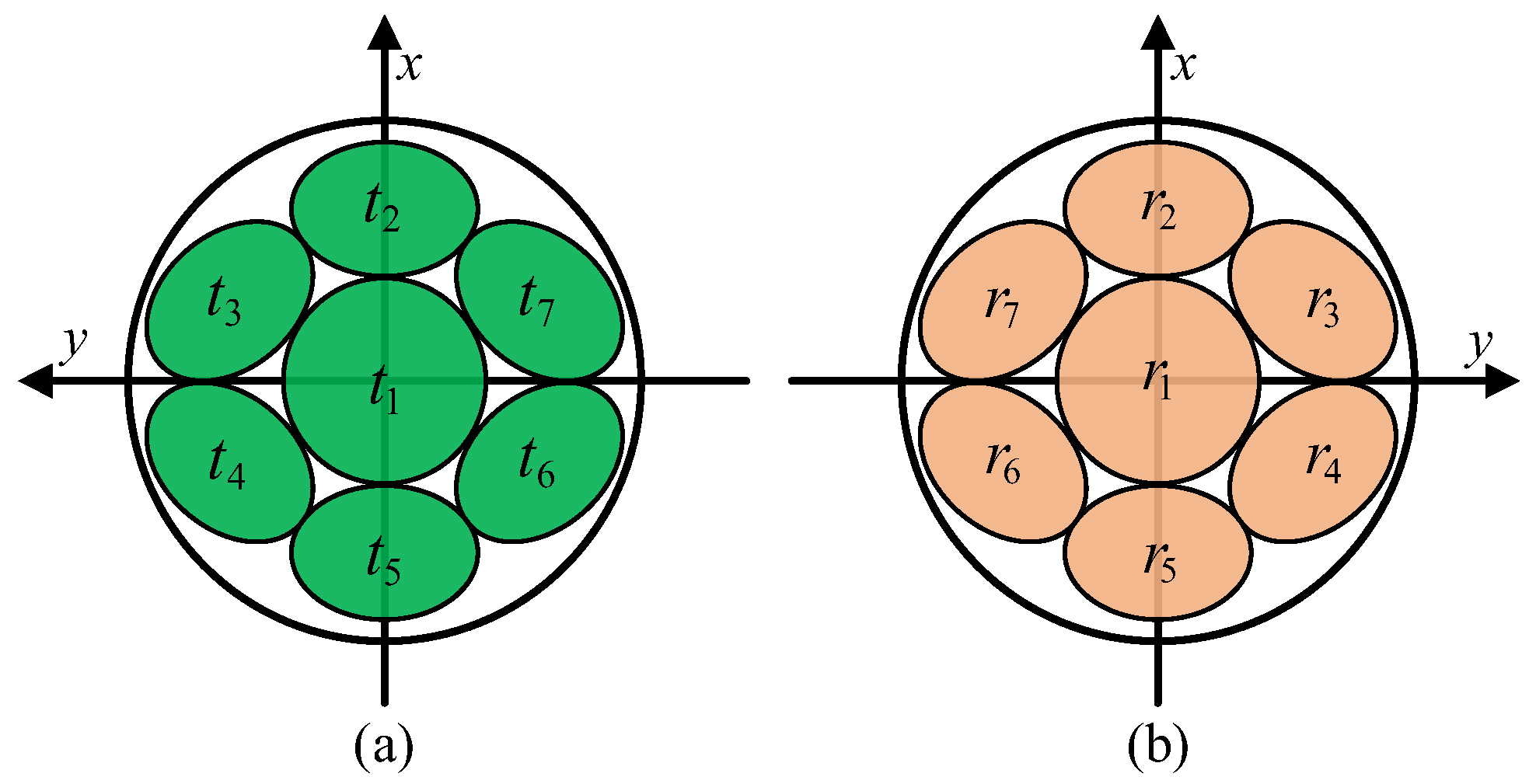
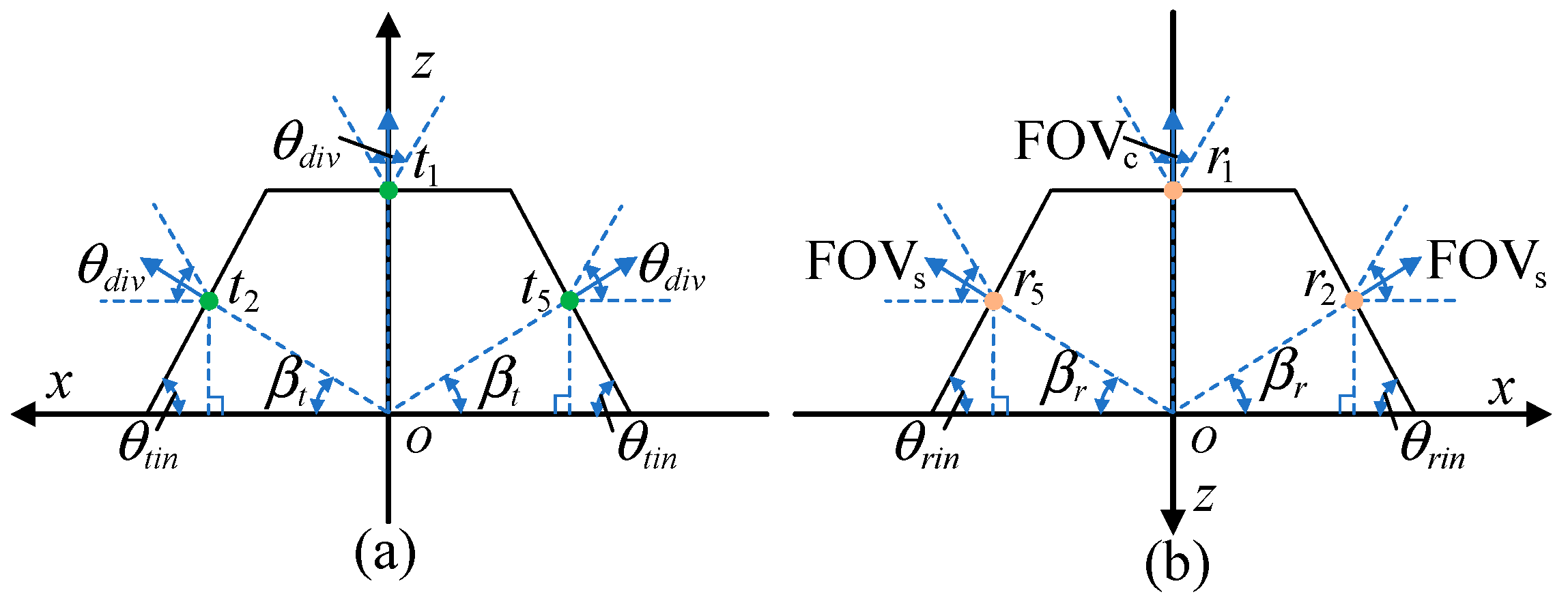
2.4. Derivation of the Transceiver Structure

Based on the above, the parameters required for designing the hemispherical transceivers can be determined. These parameters include the elevation angles ${\beta }_t$ and ${\beta }_r$, the azimuth angles ${\phi }_t$ and ${\phi }_r$, and the coordinate positions $\left(x_t^i,y_t^i,z_t^i\right)$ and $\left(x_r^j,y_r^j,z_r^j\right)$, where $1\le i=j\le n_r+1$. $n_r$ is the number of transceivers on the side.

We design the transceiver positions as shown in Figure 4, aiming to achieve a 360° planar arrangement on the xoy plane. Except for $t_1$, all transmitters are tilted at specific angles, with their normal vectors pointing in the positive direction of the z-axis, to realize the three-dimensional structure of the transmitters. The structure of the receivers is similar to that of the transmitters.

Next, the derivation of the angular parameters is performed. It should be noted that the transmitter $t_1$ is located at the origin of the coordinate system and is similar to a SISO communication system, so there is no need to consider its azimuth and elevation parameterization.

Based on the normal vector projection of the transmitter plane plotted in Figure 5a, the azimuthal angle can be expressed as follows:

$${\phi }_t^i=(i-2){\displaystyle \frac{360°}{n_r}},$$

(7)

where $2\le i\le n_r+1$. To ensure efficient use of each side transmitter, we define the transmitter plane inclination angle as ${\theta }_{tin}$, such that the lower boundary of the beam divergence angle ${\theta }_{div}$ is parallel to the transmitter plane, as shown in Figure 6a. The transmitter plane inclination can be expressed as follows: ${\theta }_{tin}={\displaystyle \frac{180°-{\theta }_{div}}{2}}.$ According to the definition of the elevation angle, it can be derived from ${\theta }_{tin}$ as follows:

$${\beta }_t=90°-{\theta }_{tin}·$$

(8)

According to Figure 5b, it is evident that the receiver angle parameter derivation is similar to the transmitter angle parameter derivation. In both cases, the azimuth setting is the same, so the derivation process is not repeated here. Since the different side receivers are symmetrical about the center receiver, their elevation angles and FOVs are equal. To achieve omnidirectional coverage of the receiving plane, the plan view of the hemispherical receiver in the yoz plane needs to realize a 360° receiver plane arrangement. Therefore, the FOVs of each side receiver can be obtained as follows:

$${\mathrm{FOV}}_{\mathrm{s}}={\displaystyle \frac{360°}{n_r}}·$$

(9)

Here, the center receiver FOVc can be directly given by:

$${\mathrm{FOV}}_{\mathrm{c}}=180°-2{\mathrm{FOV}}_{\mathrm{s}}·$$

(10)

Similar to ${\theta }_{tin}$, the plane inclination angle is given by the following equation: ${\theta }_{rin}={\displaystyle \frac{180°-{\mathrm{FOV}}_{\mathrm{s}}}{2}},$ and according to the definition of the elevation angle, it can be derived from ${\theta }_{rin}$ as follows:

$${\beta }_r=90°-{\theta }_{rin}·$$

(11)

Based on the obtained transceiver angle parameters, the transceiver coordinate positions can be derived. As shown in Figure 7, $r_t$, $r_r$ are the radii of the projected circles of the transceiver center in the xoy plane, respectively. In the following, the position of the transmitter coordinates is first deduced. According to the order of the transmitter serial number, the coordinates of transmitter $t_1$$\left(x_t^1,y_t^1,z_t^1\right)$ are given as $\left(0,0,z_t^1\right)$. Through Figure 7a, the remaining transmitter x and y coordinates are obtained as follows:

$$\left\{\begin{array}{c}{x}_t^i=r_t\cos \left({\phi }_t^i\right)\\ y_t^i=r_t\sin \left({\phi }_t^i\right)\end{array}\right.·$$

(12)

After obtaining the transmitter x and y coordinates, we then derive the transmitter z coordinates. Through Figure 8a, the z-coordinate of transmitter $t_1$ is obtained as $z_t^1=A_t\sin \left({\theta }_{tin}\right)$. Due to the symmetric structure of the transmitter, in addition to transmitter $t_1$, a circle of transmitters around the symmetric arrangement of the z-coordinate and the plane inclination angle θ and elevation angle β parameter settings are the same. Thus, the z-coordinate is unified as follows:

$$z_t^i=r_t\tan {\beta }_t,$$

(13)

where $r_t=A_t\sin {\theta }_{tin}/2\tan {\beta }_t.$

Receiver coordinates are basically the same as the transmitter coordinates, only the corresponding parameters need to be modified for the receiver parameters, and the z-coordinate is adjusted to $z_r^i=L-A_r\sin {\theta }_{rin},$ where L is the communication distance.

3. Channel Capacity of Underwater Wireless Optical MIMO Communication System

We used the Monte Carlo method to perform photon tracking for simulation modeling of the UWOC system. A Monte Carlo flow chart is shown in Figure 9. The random path length can be obtained by $s=-\ln (\xi )/c,$ where c is the attenuation coefficient of light underwater, which is equal to the sum of the absorption coefficient a and the scattering coefficient b, and ${\epsilon }_s$ obeys uniform distribution in the range (0,1). The azimuthal angle satisfies a uniform distribution of $(0,2\pi )$, and the scattering angle is generated from the scattering phase function. We have chosen turbid port water $(a=0.366m^{-1},c=2.19m^{-1})$ as our water medium, because if the proposed communication system model demonstrates an improvement in channel capacity under turbid water conditions, it will achieve even better communication performance in relatively clearer water environments. At the same time, the Fournier–Forand (FF) phase function is chosen because it fits Petzold’s measurements well and is the most accurate theoretical scattering phase function with high accuracy. We set $w_{th}={10}^{-4}$. With the recorded photon weights and propagation distances, we can use them to calculate the subsequent channel impulse response (CIR).

For SISO systems, the channel impulse response (CIR) can be obtained by the following steps [17]: (1) By counting the total path length $d$ of each photon to reach the receiver, we can calculate the propagation time of the received photons by $t=d/v_{water}$, where $v_{water}$ is the speed of light in water. (2) Taking the range from the shortest propagation time of the photon $t_{\min }$ to the longest propagation time $t_{\max }$, we can divide them into equal intervals as $\left\{T_m;m=1,2,\dots \right\}$. (3) Calculating the power sum of the photons in each time interval and denoting it as $\{P_m;m=1,2,\dots \}$, the photon intensity $H_m$ can be obtained by: $H_m=P_m/S_{area},$ where $S_{area}$ is the receiver area. Generalizing this to MIMO, we get the channel matrix. Using the channel matrix, the channel capacity can be calculated, which is expressed as follows [13]:

$$C={\displaystyle {\sum }_{i=1}^q{\log }_2(1+SNR·{\lambda }_i)},$$

(14)

where $q$ is the number of non-zero eigenvalues in the H matrix, SNR is the signal-to-noise ratio, and ${\lambda }_i$ is the eigenvalue of H matrix. Following this, inverse extrapolation through the channel capacity is performed to obtain the channel matrix H. Based on the value of H, the outage probability of the communication system in this scenario can also be determined. In this paper, we fit CIR by using the Gaussian model, and its mathematical expression is as follows:

$$h_g(t)={\displaystyle {\sum }_{l=1}^{n_l}{a}_1{e}^{-{(\frac{t-b_1}{c_1})}^2}},$$

(15)

where $n_l$ is Gaussian function order, and $a_1$,$b_1$, and $c_1$ are real constants.

4. Analysis and Discussion of Data Results

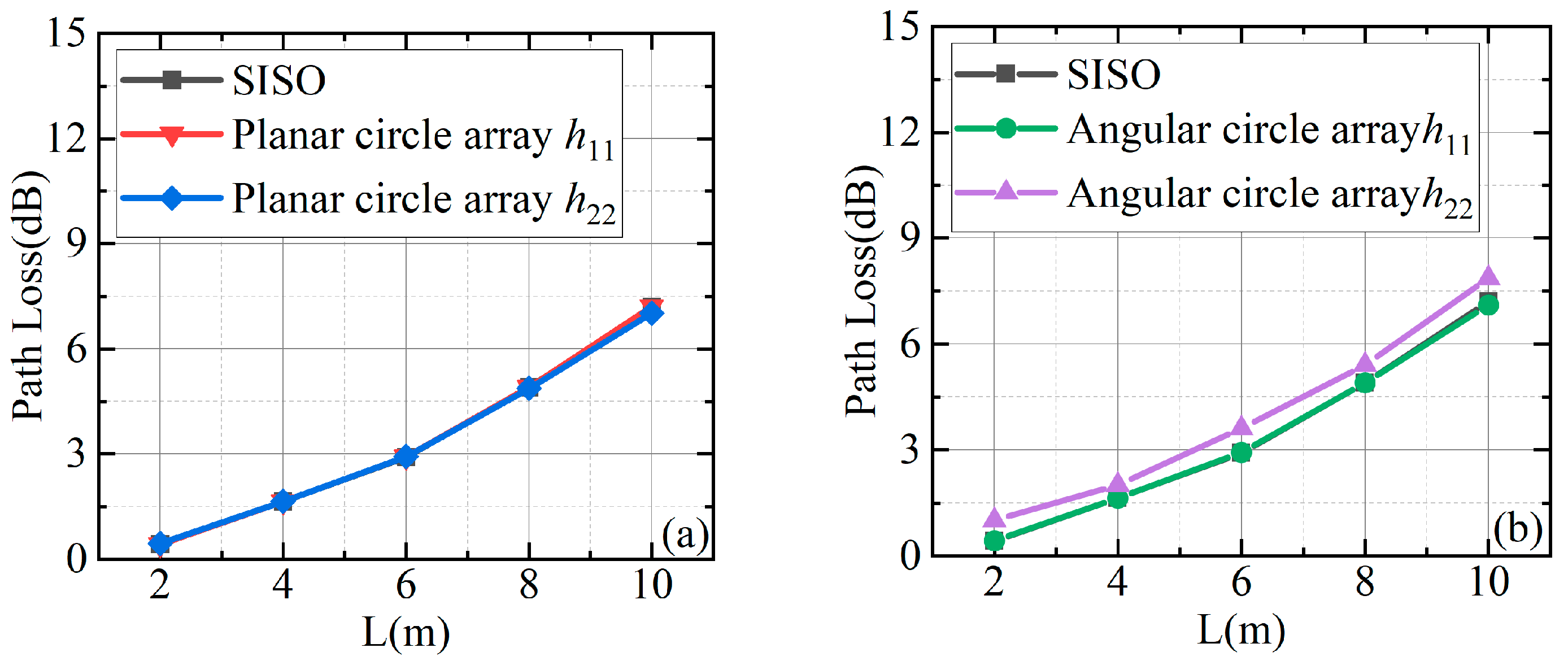
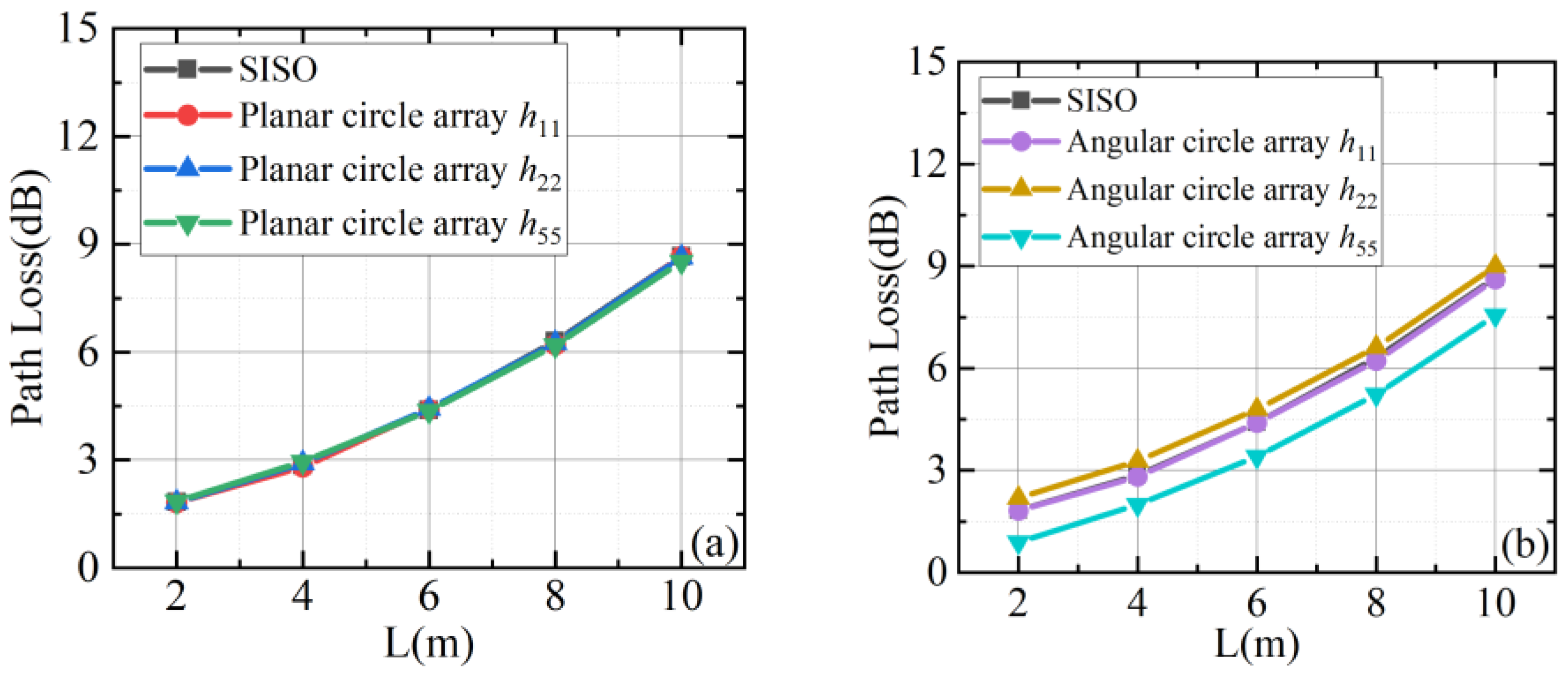
In this section, to assess the performance of UWOC for different communication distances and system settings, we study path loss, channel impulse response (CIR), function fitting, channel capacity, and outage probability. The transceiver parameters are set as shown in

Table 1. Transceiver parameters.

Parameter	Value/Unit
$\left(x_t,y_t,z_t\right)$	(0,0,0)
$P_t$	50 mw
${\theta }_{div}$	20°
$w_0$	0.001 m
$\lambda$	514 nm
$A_t$	0.15 m
$\left(x_r,y_r,z_r\right)$	$\left(0,0,L\right)$
FOV	60°
$A_r$	0.15 m

. Subsequently, we use $h_{11}$ to represent the data received by receiver 1 from transmitter 1, which encompasses path loss and CIR. Similarly, $h_{12}$ and $h_{21}$ denote the data exchanged between other transmitter–receiver pairs, though their detailed descriptions are omitted here.

4.1. Path Loss

From Figure 10, we can observe that the path loss curves for the SISO communication system and the transceiver pairs of the planar circle array, as well as the transceiver pairs at the center of the angular circle array, are essentially the same. However, the side transceiver pairs of the angular circle array experience greater path loss compared to the other structures. This is because the side transceivers of the angular circle array are tilted outward at an angle to achieve a larger communication range. This tilting breaks the LOS link, resulting in a reduction in the number of photons received and consequently increasing the path loss.

Next, the non-line-of-sight (NLOS) case is considered. From Figure 11, we can observe that the path loss at the same communication distance for all system settings is greater than that for the LOS link. This increase in path loss is due to the break in the transceiver alignment link caused by the deflection. From Figure 10, we can also observe that the path loss for the transceiver pair $T_5-R_5$ of the angular circle MIMO communication system is less than that of other transceiver pairs and is close to the path loss in the line-of-sight case. This is attributed to the unique structure of the angular circle MIMO system, where the side transceivers are outward at a certain inclination angle, mitigating the effect of the NLOS link.

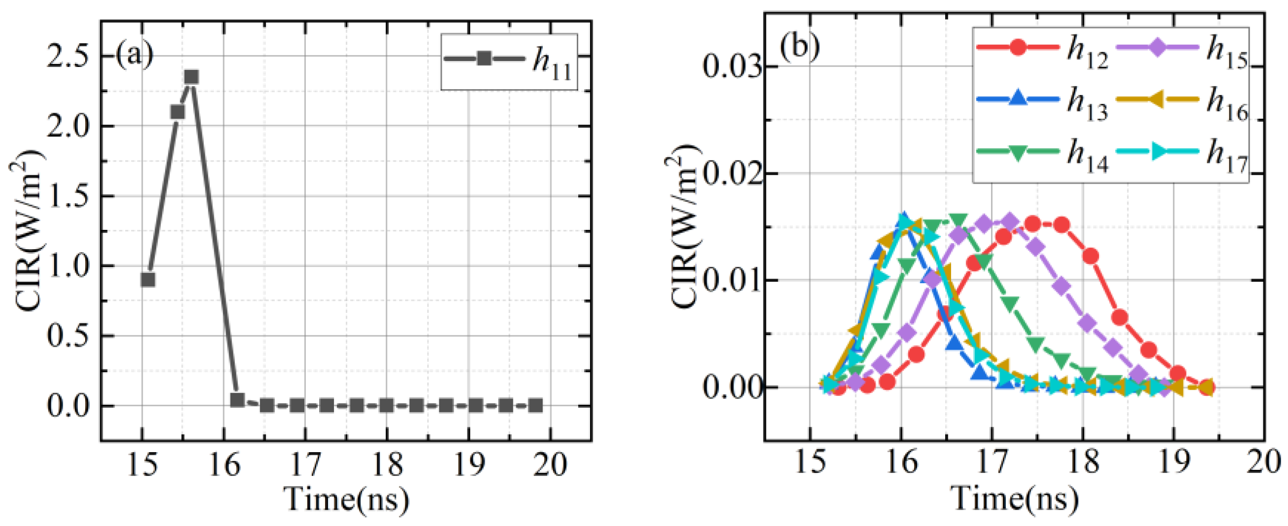
4.2. Channel Impulse Response

From Figure 12 and Figure 13, we can observe that the CIR intensity for $t_1(t_2)$−the other receivers is very slow, whereas the CIR intensity for $t_1(t_2)$−$r_1(r_2)$ is very high. The data show that the photons emitted by $t_1(t_2)$ in the planar circle array MIMO communication system are almost received by $r_1(r_2)$ with only a small portion captured by other receivers. This is because, in the transceiver structure of the planar circle array MIMO communication system, $t_1(t_2)$ and $r_1(r_2)$ are perfectly aligned. Moreover, as seen in Figure 12b, the CIR curve for $t_1$ to the other receivers shows consistent temporal broadening and intensity. This is because the other receivers are symmetrically distributed with respect to $r_1$. In Figure 13b, we found that the CIR curve for $t_2$−$r_4,r_5,r_6$ disappears. This is because $r_4$, $r_5$, and $r_6$ are located on the negative x-axis, far from $t_2$ and basically do not receive any photons, hence the CIR cannot be obtained through statistical methods.

Comparing Figure 12 and Figure 14, it can be seen that the CIR curves for transceiver 1 are almost identical in both system configurations. This is because the central transceiver pair in the angular circle array MIMO communication system is aligned. Although the side receivers of the angular circle array MIMO communication system are inclined outward at a certain angle, the short communication distance results in little change in the number of received photons, hence the CIR intensity for $T_1$−the other receivers do not change significantly. In the case of longer distance communication, the special structure of the angular circle array MIMO communication system makes the CIR intensity for $T_2$−the other receivers decrease. Comparing Figure 13 and Figure 15, it can be seen that transceiver 2 has less CIR intensity in the angular circle array MIMO communication system setup. This is because transmitter $T_2$ and the receivers are inclined outward at a certain angle, breaking the LOS link and resulting in fewer received photons.

4.3. Function Fitting

In this paper, a Gaussian function is used to fit the CIR data of MIMO communication systems with different system settings. From Figure 16 and Figure 17, we can observe that the CIR data obtained from both planar circular array MIMO communication system and angular circular array MIMO communication system are well fitted with the Gaussian function.

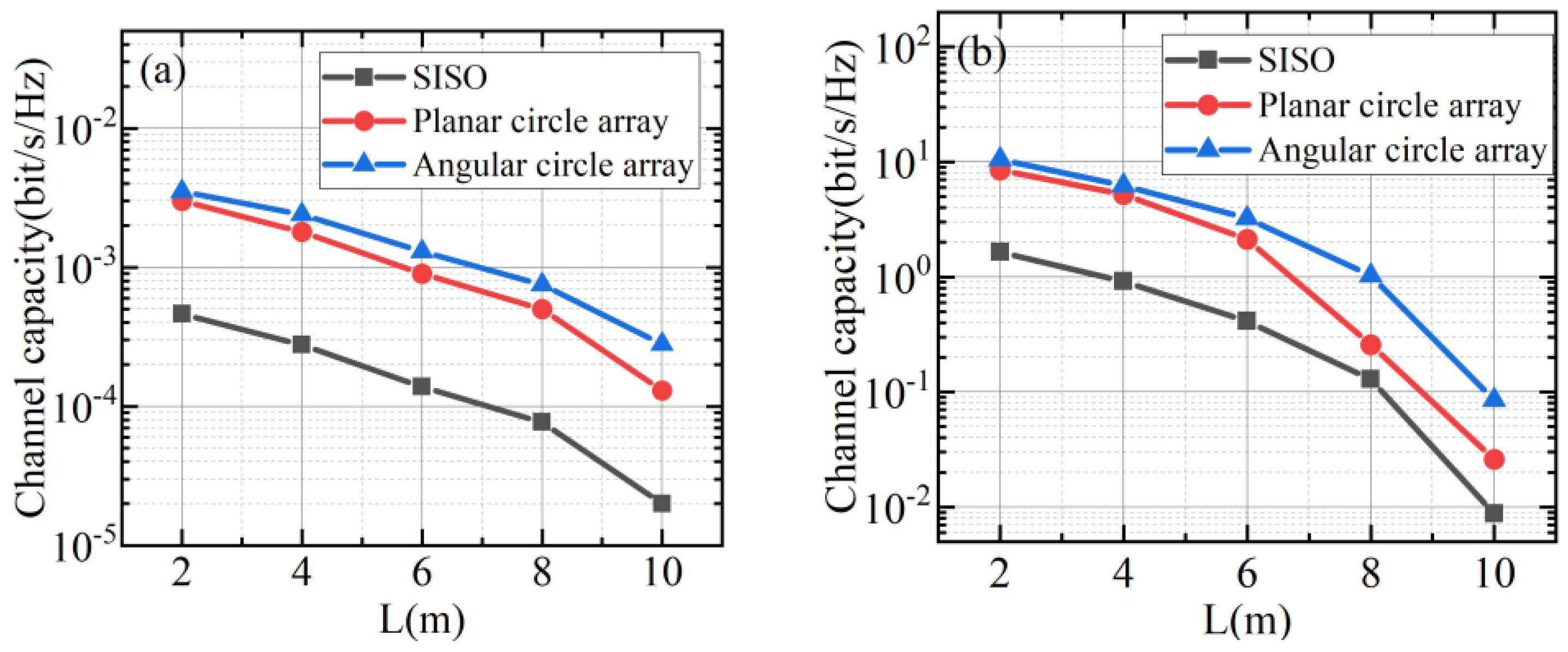
4.4. Channel Capacity

The SNR at the receiving end can reach between a few dB and tens of dB; in this paper, we choose the two conditions of small SNR: 5 dB and large SNR: 40 dB, respectively. As shown in Figure 18, the channel capacity of the planar circle array MIMO communication system is slightly larger than that of the angular circle array MIMO communication system, while the channel capacity of the SISO communication system is significantly smaller than that of the other two systems. At 5 dB and a communication distance of 10 m, our system achieves a channel capacity improvement of 6.64 dB compared to the SISO system. At 40 dB and a communication distance of 10 m, our system achieves a channel capacity improvement of 6.73 dB compared to the SISO system. This is because MIMO communication systems have a larger number of transceivers, resulting in more photons being emitted, which increases the channel capacity. However, in the angular circle array MIMO system, many transceivers have angular offset settings, and the path loss for the side transceiver pairs is greater. Therefore, the channel capacity is lower than that of the planar circle array MIMO communication system at the LOS link.

Comparing Figure 18 and Figure 19, it can be seen that the channel capacity is reduced for all communication systems under the same SNR condition with transmitter deflection. At 5 dB and a communication distance of 10 m, our system achieves a channel capacity improvement of 13 dB compared to the SISO system. At 40 dB and a communication distance of 10 m, our system achieves a channel capacity improvement of 10 dB compared to the SISO system. This reduction is due to the transmitter deflection breaking the LOS link, resulting in fewer photons being received, an increase in path loss, and hence a reduction in channel capacity. Additionally, we can observe that the channel capacity of the angular circle array MIMO communication system is greater than that of the planar circle array MIMO communication system when the transmitter is deflected. This is because the special structural design of the angular circle array MIMO system mitigates the path loss caused by NLOS links.

4.5. Outage Probability

We assume that a link outage occurs when the channel capacity per unit bandwidth is less than one. Corresponding to the graph where the path loss is less than the green line, the communication system is considered to operate normally. From this, the system outage probability can be calculated. In Figure 20a, the outage probabilities of the planar circle array system and the angular circle array system are 75% and 89%, respectively. In Figure 20b, the outage probabilities are 82% and 100%, respectively. In Figure 20c, the outage probabilities are 69% and 76%, respectively. The data show that the proposed system is superior to the planar circle array communication system in different mobile scenarios. Moreover, when only the angle of the transceiver changes, the performance optimization of this system is more evident.

5. Conclusions

In this paper, we propose the angular circle array MIMO scheme, which systematically enhances the ability to establish and maintain communication links without adding extra following systems, thereby improving channel capacity. Our proposed scheme has less path loss under NLOS links and achieves significant improvements in channel capacity compared to both the planar circle array MIMO communication system and the SISO communication system. Our scheme can be used for ocean observation, submarine volcano early warning, and ocean oil and gas exploration. In the future, we will conduct experimental verification of a real underwater optical communication channel.

References

1. Qu, F.; Wang, Z.; Yang, L.; Wu, Z. A journey toward modeling and resolving doppler in underwater acoustic communications. IEEE Commun. Mag. 2016, 54, 49–55. [Google Scholar] [CrossRef]
2. Fornari, D.J.; Bradley, A.; Humphris, S.E.; Walden, B.; Deuster, A. Inductively coupled link (ICL) temperature probes for hot hydrothermal fluid sampling from ROV Jason and DSV Alvin. Ridge Events 1997, 8, 26–30. [Google Scholar]
3. Palmeiro, A.; Martín, M.; Crowther, L.; Rhodes, M. Underwater radio frequency communications. In Proceedings of the OCEANS 2011 IEEE-Spain, Santander, Spain, 6–9 June 2011. [Google Scholar]
4. Chowdhury, M.Z.; Hossan, M.T.; Islam, A.; Jang, Y.M. A comparative survey of optical wireless technologies: Architectures and applications. IEEE Access 2018, 6, 9819–9840. [Google Scholar] [CrossRef]
5. Hanson, F.; Radic, S. High bandwidth underwater optical communication. Appl. Opt. 2008, 47, 277–283. [Google Scholar] [CrossRef] [PubMed]
6. Wang, J.; Lu, C.; Li, S.; Xu, Z. 100 m/500 Mbps underwater optical wireless communication using an NRZ-OOK modulated 520 nm laser diode. Opt. Express 2019, 27, 12171–12181. [Google Scholar] [CrossRef] [PubMed]
7. Hu, F.; Li, G.; Zou, P.; Hu, J.; Chen, S.; Liu, Q. 20.09-Gbit/s Underwater WDM-VLC transmission based on a single Si/GaAs-substrate multichromatic LED array chip. In Proceedings of the 2020 Optical Fiber Communications Conference and Exhibition (OFC), San Diego, CA, USA, 8–12 March 2020. [Google Scholar]
8. Fei, C.; Wang, Y.; Du, J.; Chen, R.; Lv, N.; Zhang, G.; Tian, J.; Hong, X.; He, S. 100-m/3-Gbps underwater wireless optical transmission using a wideband photomultiplier tube (PMT). Opt. Express 2022, 30, 2326–2337. [Google Scholar] [CrossRef] [PubMed]
9. Chen, Z.; Liu, Y.; Yi, X.; Zhao, R. Design and Simulation of Underwater Wireless Optical Angular Circle Array MIMO Communication Systems. In Proceedings of the 2024 IEEE 10th International Conference on Underwater System Technology: Theory and Applications, Xi’an, China, 18–20 October 2024. [Google Scholar]
10. Zeng, Z.; Fu, S.; Zhang, H.; Dong, Y.; Cheng, J. A survey of underwater optical wireless communications. IEEE Commun. Surv. Tutor. 2017, 19, 204–238. [Google Scholar] [CrossRef]
11. Ramavath, P.N.; Udupi, S.A.; Krishnan, P. High-speed and reliable underwater wireless optical communication system using multiple-input multiple-output and channel coding techniques for IoUT applications. Opt. Commun. 2020, 461, 125229–125235. [Google Scholar] [CrossRef]
12. Ata, Y.; Baykal, Y.; Gökçe, M.C. Analysis of optical wireless MIMO communication in underwater medium. IEEE Internet Things J. 2024, 11, 20660–20672. [Google Scholar] [CrossRef]
13. Dong, Y.; Liu, J.; Zhang, H. On capacity of 2-by-2 underwater wireless optical MIMO channels. In Proceedings of the 2015 Advances in Wireless and Optical Communications (RTUWO), Riga, Latvia, 5–6 November 2015. [Google Scholar]
14. Jamali, M.V.; Salehi, J.A.; Akhoundi, F. Performance studies of underwater wireless optical communication systems with spatial diversity: MIMO scheme. IEEE Trans. Commun. 2017, 65, 1176–1192. [Google Scholar] [CrossRef]
15. Cox, W.C., Jr. Simulation, Modeling, and Design of Underwater Optical Communication Systems; North Carolina State University: Raleigh, NC, USA, 2012. [Google Scholar]
16. Ying, L.Z.; Ying, M.W.; Ai, P.H. Analysis of Underwater Laser Transmission Characteristics Under Monte Carlo Simulation. In Proceedings of the 2018 OCEANS-MTS/IEEE Kobe Techno-Oceans (OTO), Kobe, Japan, 28–31 May 2018. [Google Scholar]
17. Yi, X.; Liu, J.; Liu, Y.; Ata, Y. Monte-Carlo based vertical underwater optical communication performance analysis with chlorophyll depth profiles. Opt. Express 2023, 31, 41684–41700. [Google Scholar] [CrossRef] [PubMed]
Figure 1. Three-dimensional structure of transceivers in the underwater wireless optical communication system: (a) SISO system, (b) planar circle array, and (c) angular circle array.
Photonics 12 00012 g001
Figure 2. Transceiver parameters in the angular circle array MIMO system.
Photonics 12 00012 g002
Figure 3. Schematic diagram of the receiver plane and photon scattering.
Photonics 12 00012 g003
Figure 4. Projection diagram of the angular circle array MIMO communication system on the xoy plane: (a) transmitters and (b) receivers.
Photonics 12 00012 g004
Figure 5. Projection diagram of the transceiver plane normal vectors of the angular circle array MIMO communication system on the xoy plane: (a) transmitters and (b) receivers.
Photonics 12 00012 g005
Figure 6. Geometric structure of the angular circle array MIMO communication system in the zox cross-section: (a) transmitters and (b) receivers.
Photonics 12 00012 g006
Figure 7. Transceiver xoy plan view of angular circle array MIMO communication system: (a) transmitters and (b) receivers.
Photonics 12 00012 g007
Figure 8. Transceiver cross-section diagram of the angular circle array MIMO communication system: (a) transmitters and (b) receivers.
Photonics 12 00012 g008
Figure 9. Monte Carlo flow chart.
Photonics 12 00012 g009
Figure 10. Path loss under different communication system settings in the LOS link: (a) planar circle array and (b) angular circle array.
Photonics 12 00012 g010
Figure 11. Path loss under different communication system settings for transmitter deflection: (a) planar circle array and (b) angular circle array.
Photonics 12 00012 g011
Figure 12. CIR curves of transceiver 1 in the planar circle array MIMO communication system when L = 2 m : (a) t 1 r 1 and (b) t 1 −the other receivers.
Photonics 12 00012 g012
Figure 13. CIR curves of transceiver 2 in the planar circle array MIMO communication system when L = 2 m : (a) t 2 r 2 and (b) t 2 −the other receivers.
Photonics 12 00012 g013
Figure 14. CIR curves of transceiver 1 in the angular circle array MIMO communication system when L = 2 m : (a) T 1 R 1 and (b) T 1 −the other receivers.
Photonics 12 00012 g014
Figure 15. CIR curves of transceiver 2 in the angular circle array MIMO communication system when L = 2 m : (a) T 2 R 2 and (b) T 2 −the other receivers.
Photonics 12 00012 g015
Figure 16. CIR fitting for planar circle array MIMO communication system when L = 2 m : (a) h 11 , h 22 and (b) h 12 , h 21 .
Photonics 12 00012 g016
Figure 17. CIR fitting for angular circle array MIMO communication system when L = 2 m : (a) h 11 , h 22 and (b) h 12 , h 21 .
Photonics 12 00012 g017
Figure 18. Channel capacity of different communication system settings under different SNR levels at the LOS link: (a) 5 dB and (b) 40 dB.
Photonics 12 00012 g018
Figure 19. Channel capacity of different communication system settings under different SNR levels when the transmitter is deflected: (a) 5 dB and (b) 40 dB.
Photonics 12 00012 g019
Figure 20. Path loss under different communication system settings in a mobile scenario: (a) position, (b) angle, and (c) position + angle.
Photonics 12 00012 g020