Abstract
Overlay accuracy, one of the three fundamental indicators of lithography, is directly influenced by alignment precision. During the alignment process based on the Moiré fringe method, a slight angular misalignment between the mask and wafer will cause the Moiré fringes to tilt, thereby affecting the alignment accuracy. This paper proposes a leveling strategy based on the DQN (Deep Q-Network) algorithm. This strategy involves using four consecutive frames of wafer tilt images as the input values for a convolutional neural network (CNN), which serves as the environment model. The environment model is divided into two groups: the horizontal plane tilt environment model and the vertical plane tilt environment model. After convolution through the CNN and training with the pooling operation, the Q-value consisting of n discrete actions is output. In the DQN algorithm, the main contributions of this paper lie in three points: the adaptive application of environmental model input, parameter optimization of the loss function, and the possibility of application in the actual environment to provide some ideas. The environment model input interface can be applied to different tilt models and more complex scenes. The optimization of the loss function can match the leveling of different tilt models. Considering the application of this strategy in actual scenarios, motion calibration and detection between the mask and the wafer provide some ideas. To verify the reliability of the algorithm, simulations were conducted to generate tilted Moiré fringes resulting from tilt angles of the wafer plate, and the phase of the tilted Moiré fringes was subsequently calculated. The angle of the wafer was automatically adjusted using the DQN algorithm, and then various angles were measured. Repeated measurements were also conducted at the same angle. The angle deviation accuracy of the horizontal plane tilt environment model reached 0.0011 degrees, and the accuracy of repeated measurements reached 0.00025 degrees. The angle deviation accuracy of the vertical plane tilt environment model reached 0.0043 degrees, and repeated measurements achieved a precision of 0.00027 degrees. Moreover, in practical applications, it also provides corresponding ideas to ensure the determination of the relative position between the mask and wafer and the detection of movement, offering the potential for its application in the industry.
1. Introduction
Overlay accuracy is the key factor affecting the productivity of lithography machines [1]. Before performing the overlay process in lithography, it is necessary to determine the alignment between the lithography mask and wafer, and the alignment precision is approximately one-third of the overlay accuracy [2]. The alignment method based on the Moiré fringe is a current research hotspot in alignment systems due to its advantages of a simple measurement optical path and high measurement accuracy [3,4,5,6,7]. During the alignment process, a slight angular misalignment between the mask and wafer will cause the generated Moiré fringe to tilt, thereby affecting the alignment accuracy. Therefore, achieving leveling of the mask and wafer is currently a key research focus.
Zhu et al. [8,9,10] analyzed the influencing factors causing tilted Moiré fringes, and their experiments proved that varying tilt angles have distinct effects on alignment accuracy. They proposed two methods for correcting a tilted Moiré fringe; one is based on Moiré fringe phase analysis correction, and the other is a spatial frequency decomposition method, but both methods achieve nanometer-level correction. Zhou et al. [11,12] proposed a tilt-modulated spatial phase imaging method to adjust the inconsistency in the wafer–mask leveling gap. On this basis, they proposed a Moiré-based phase-sensitive imaging scheme to sense and adjust the in-plane twist angle; this method is sufficient for many practical applications and provides an idea for the highly sensitive detection of the in-plane twist angle between two parallel planes. Xing et al. [13] proposed a digital rotation Moiré (DRM) method for strain measurement based on high-resolution transmission electron microscope lattice images; the proposed method, based on the rotational Moiré principle and a digital Moiré algorithm, detects in-plane strain components by quantifying image parameters. The leveling accuracy of these methods is very high. However, traditional methods for leveling tilted Moiré fringe images one by one require a significant amount of computing time and human effort, which does not align with the current alignment development needs.
Wang et al. [14,15] proposed a one-step misalignment regression measurement strategy based on deep learning, which achieved sub-nanometer misalignment measurement accuracy on the alignment marks of micron-level circular gratings and line gratings through the use of deep neural networks. It was also shown to be robust against manufacturing defects, environmental noise, alignment variations, and systematic errors. However, the author’s current research does not utilize deep learning to correct tilted Moiré fringes. Mnih et al. [16] proposed the concept of deep reinforcement learning combining deep learning and reinforcement learning to implement an end-to-end algorithm from perception to action. They established a Deep Q-Network (DQN) model to achieve the result of playing Atari games solely from image input through agent learning. Due to the strong versatility of this model, many scholars have applied this model to various fields. Devo et al. [17] used the DQN model in deep reinforcement learning to generalize target-driven visual navigation. Two networks were designed: one is the target network, and the other is the positioning network. They work together to explore the environment and locate the target. Ngan et al. [18] conducted a detailed review of the concept of deep reinforcement learning and its application in various fields, with a primary focus on computer vision. Their review covered topics such as landmark localization, object detection, object tracking, registration on two-dimensional and three-dimensional image volumetric data, and image segmentation. Additionally, the authors provided a detailed analysis of other aspects and discussed the future directions of deep reinforcement learning. Therefore, the research direction of integrating disciplines across multiple fields aligns more closely with the current development trends in industry and academia.
Compared with the traditional Moiré fringe analysis algorithm [8,9,10,11,12,13], using the DQN algorithm to automatically adjust the status of the mask and wafer will consume less time and energy. This paper is inspired by the different applications of this algorithm in various fields [19,20,21,22]. Some parameter adjustments were made to the algorithm so that the adjustment strategy combined with the algorithm can adapt to more complex environments. The main contribution of this paper is to first adjust the loss function of the algorithm and the environmental input window model. Secondly, in the CNN, the Moiré fringe image phase analysis module is incorporated to enable the algorithm to resolve the mask and wafer tilt model. It can also address the Moiré fringe image phase, achieving a small gap in the accuracy of the solution error between the two. Finally, in order to be close to practical applications, the algorithm considers the accuracy of motion calibration and state detection between the actual mask and wafer.
This paper proposes a mask and wafer leveling theory based on the DQN algorithm. It enhances the method of leveling the wafer angle through theoretical calculations and utilizes the interaction between the CNN-Behavior network and the environmental state (i.e., the horizontal plane tilt environment model and the vertical plane tilt environment model) for training. This approach achieves the automatic leveling of Moiré fringes, addressing the issue of tilt between the mask and wafer, which impacts the phase analysis of the Moiré fringe.
2. Strategic Analysis
2.1. Tilted Moiré Fringe Alignment Principle
During the alignment process between the mask and wafer, a Moiré fringe is formed when the wafer is tilted relative to the mask, leading to changes. When the grating mark on the mask rotates and tilts within the plane relative to the grating mark on the wafer, the Moiré fringe formed by the two gratings will exhibit a certain degree of inclination. Similarly, when the two gratings rotate and tilt in space, the Moiré fringe formed by them will exhibit a certain degree of inclination and frequency variation. These inclinations will result in an inability to extract phase information from the Moiré fringe, thereby affecting the final alignment accuracy. Zhou et al. [11,12] elucidated the basic principles of Moiré fringe phase analysis. Building upon this foundation, this paper provides a simple analysis of the tilting process between the wafer and mask.
As shown in Figure 1a, when illuminated by a 365 nm ultraviolet light source, a Moiré fringe is formed by the displacement between the alignment marks on the mask and the wafer. The alignment marks on the upper-quadrant line grating mask have a period of 4 μm, and those on the lower-quadrant line grating have a period of 4.4 μm; the alignment marks on the mask and wafer are in a parallel misalignment state.
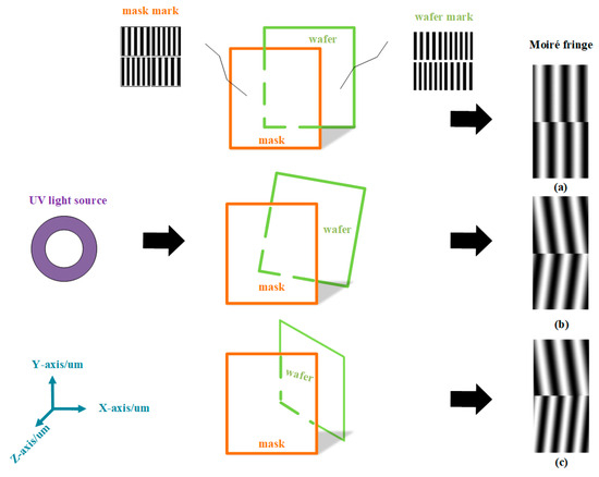
Figure 1.
The distribution of the two sets of fringes varies depending on the tilt of the wafer in different scenarios: (a) when the wafer is leveled, (b) when the wafer is tilted in the horizontal direction, and (c) when the wafer is tilted in the vertical direction.
The light field distribution of the Moiré fringe can be expressed as
Here, and represent the interference intensity of the upper and lower parts of the Moiré fringe, respectively; and represent the intensity of the background light; and and represent the periods of the mask alignment mark and wafer alignment mark, respectively.
As shown in Figure 1b, when in the x–y section, the wafer is tilted in the horizontal plane, and the light field distribution of the Moiré fringe can be expressed as
Here, and represent the interference intensity of the tilted in horizontal plane Moiré fringe, respectively; represents the wafer and mask forming an angular deviation of within the horizontal plane. The negative sign represents the opposite directions of the upper tilt and the lower tilt. The angular deviation can be determined from other misalignments, including the offsets between the centers of the mask and wafer alignment marks, and can be expressed as
Here, represents the antisine function, and represents the offsets between the centers of the mask and wafer alignment marks. represents the distance between the centers of the horizontally aligned line gratings on a mask mark or wafer mark.
As shown in Figure 1c, when the wafer is tilted in the x–z section, the wafer is tilted in the vertical plane, and the light field distribution of the Moiré fringe can be expressed as
Here, and represent the interference intensity of tilted in vertical plane Moiré fringe, respectively; represents the fringe frequency change caused by the tilt of the wafer relative to the mask in the vertical plane; and represents the tilt of the wafer relative to the mask in the vertical plane causing changes in the stripe angle . The negative sign represents the opposite directions of the upper tilt and the lower tilt. The stripe angle and the fringe frequency can be expressed as
Here, represent the rotation angle due to the tilt of the wafer relative to the mask in the vertical plane; and represent the diffraction angles of the mask alignment mark and the wafer alignment mark, respectively; represents the wavelength of the light source; represents the tilt angle in the vertical plane; and represents the original frequency.
Changes in the relative positions of the mask and wafer directly reflect alterations in the Moiré fringe. Therefore, the relative positions of the mask and wafer are simply divided into two parts: the horizontal plane (x–y direction) and the vertical plane (x–z direction). This is basically used to establish a simulated tilt model, which consists of a set of mask and wafer tilt pictures. This is used as the input value for the convolutional neural network and incorporated into the DQN algorithm for training.
2.2. Tilted Moiré Fringe Leveling Strategy
In the Moiré fringe alignment method, when the mask and wafer are tilted, the resulting Moiré image will also be tilted. Generally speaking, the mask is created by numerically analyzing the tilted Moiré fringe. Unlike previous leveling processes between the mask and wafer [8,9,10,11,12,13], our proposed method simulates the tilting state between the mask and wafer, as illustrated in Figure 2. The input consists of four sets of mask and wafer pictures depicting various tilt states as the environmental condition. The picture size is 80 × 80, and four frames are grouped together. The four frames of data are just the initial input data, which is continuously iterated. Initial data are input to CNN-Behavior network training and stored in the experience replay pool. Subsequently, new initial data is taken from the experience pool to replace the original initial data training. In other words, the status between the mask and the wafer is continuously updated during the training process. This enables automatic leveling of the mask and wafer. Since convolutional neural networks (CNNs) excel at modeling complex functions, we utilize a CNN as a function approximator to estimate the Q-value. Essentially, when a state is input, the CNN outputs the Q-values corresponding to all currently executable actions. The Q-value serves as the input value for the Deep Q-Network (DQN) algorithm. The DQN algorithm consists of three main components [16]: the CNN-Behavior network, the CNN-Target network, and the experience replay pool. The CNN-Behavior network is responsible for training the Q-value output by the CNN to produce the optimal state-action value for the agent. The role of the experience replay pool is to interact with various environmental states. After the data are generated, a batch of samples is randomly selected from the data to train the CNN-Behavior network and the CNN-Target network. The initial parameter settings of the CNN-Target network and the CNN-Behavior network are exactly the same. At certain time intervals, the parameters of the CNN-Behavior network are updated and copied to the CNN-Target network. This process helps to maintain the stability of the target Q-value over a short period of time. The overall idea of the DQN algorithm is to observe for a period of time before training the Q-value, collect the data into an experience replay pool, and then use this pool as the training sample data. The number of samples used for training is randomly selected. After the CNN-Behavior network obtains the best action behavior Q-value and interacts with the environmental state, the mask and wafer determine the next action. Then, the next frame information is acquired, the picture is updated, four frames of pictures are compiled as the next state, and the current state is updated. Each cycle generates an optimal action behavior Q-value and then interacts with the environment. The mask and wafer then execute the best action. By connecting these actions in series, the mask and wafer can be automatically leveled.
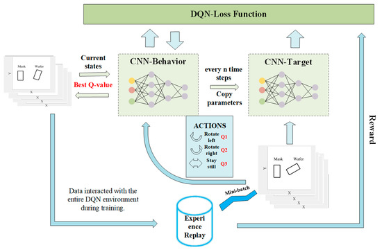
Figure 2.
System flow chart for leveling a tilted Moiré fringe via a DQN.
2.3. Network Architecture and Training Methodology
As shown in Figure 3, the CNN-Behavior network structure is based on a convolutional neural network. The network comprises three convolutional layers, one pooling layer, three activation layers, and two fully connected layers. Each operation follows batch normalization and does not require zero padding. The activation layer utilizes the ReLU function, which introduces nonlinearity to matrix operations. In the figure, for the first convolutional layer, 8 × 8 indicates that the size of each filter in the layer is 8 pixels by 8 pixels, 4 indicates that there are four channels in the input data being convolved and indicates that there are 32 filters in this convolutional layer.
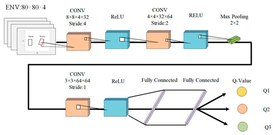
Figure 3.
CNN-Behavior network architecture.
For each convolutional layer, the number of filters is as follows: 32, 64, and 64. A maximum pooling layer (2 × 2, stride 2) is used to reduce the number of parameters, avoid overfitting, and increase the processing speed of the model. Following the last convolutional layer, there are two fully connected layers with units of 512 and 3, respectively. The network uses four-channel 80 × 80 wafer tilt images as the input, and the output is the Q-value represented by all actions.
To train the network, the first step is to initialize the experience replay pool as a queue D with a capacity of N. As shown in Figure 4, the experience replay pool selects an action using the ε-greedy strategy [16]. After execution, the system obtains rewards and the next state from the environment, and it then combines the reward function, action, and current state. The latest statuses are stored as training samples, and then a batch of samples is randomly selected for disrupted training. The ε-greedy strategy can be expressed as
where represents the Q-value of the best action, s represents a state, and a represents an action.
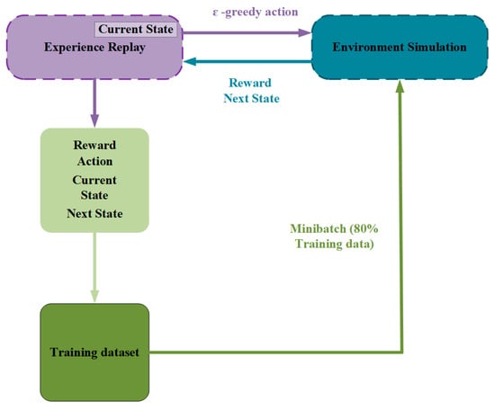
Figure 4.
Operating principle of the experience replay pool.
The second step is to randomly initialize the weight of the CNN-Behavior network Q and the weight of the CNN-Target network Q. The functions of these two networks are different. The CNN-Behavior network is responsible for controlling the mask and wafer leveling, collecting experience, while the CNN-Target network is used to calculate the TD target. Then, data randomly taken from the experience replay pool are used to calculate the target value of the CNN-Target network. The calculation formula can be expressed as
where represents the actual observed current state value; represents the discount factor, which also represents the long-term expected return of taking action in state s; represents the next state; and represents the estimate made by the CNN-Target network at . The Q-value must be maximized each time an action is selected.
During the update process, only the weight of the CNN-Behavior network is updated, while the weight of the CNN-Target network remains unchanged. After a certain number of updates, the updated weight of the CNN-Behavior network is copied to CNN-Target network for the next batch of updates. The CNN-Target network completes the update at this time. Since the target value returned is relatively fixed during a period of time when the CNN-Target network does not change, the introduction of the target network enhances the learning stability.
As shown in Figure 5, the loss function is calculated next. By continuously calculating the residual between the predicted value and the actual value, the parameters of the training model are constantly updated. This process leads to a reduction in the residual value, which gradually converges to a stable value to obtain the best training parameter model.
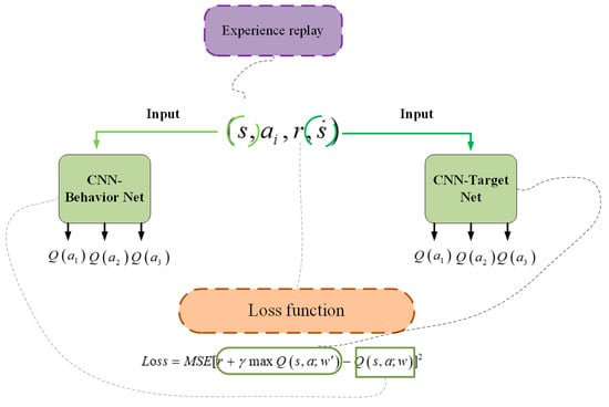
Figure 5.
Loss function calculation principle in the DQN algorithm.
The loss function can be expressed as
The goal is to minimize the loss function by using the gradient descent method through backpropagation of the CNN-Behavior network to update the weight of the CNN-Behavior network. The gradient descent method is specifically expressed as the following formula:
Here, represents the updated weight, represents the learning rate, and represents the derivative with respect to in , used to obtain the factors. From the steps outlined above, a four-tuple transition can be obtained: After training, the data are stored in the experience replay pool; then, sample data are randomly extracted from the experience replay pool, and the update process described above is repeated. The entire process is mainly based on the Deep Q-Network (DQN) algorithm outlined in Algorithm 1.
| Algorithm 1: DQN algorithm flow in mask–wafer leveling simulation. | |
| Step 1: | Initialize experience replay pool D to capacity N; |
| Step 2: | Initialize CNN-Behavior network with random weights , Initialize CNN-Target network with random weights = ; |
| Step 3: | For episode = 1, M do Initialize sequence , and preprocessed sequence ; For t = 1, T do
End For |
The CNN-Behavior network and CNN-Target network were implemented on a hardware setup including a 32-core AMD Ryzen Thread ripper PRO 5975WX (3.6 GHZ), 512 GB of RAM, and 12×NVIDIA RTX A5000 GPUs.
Simulation conditions: Extract data from the queue of the experience replay pool and organize them into batches of 32 data points. Each batch should include the current state, actions, rewards corresponding to the actions, and the subsequent state. Calculate the current state value based on the Bellman equation [16] and store it in the experience replay pool. Send the batch data (comprising the current state, action, reward corresponding to the action, and next state) to the CNN-Behavior network structure for training. The network uses GPU training to update the weight parameter matrix. In this case, for the CNN-Behavior network, the learning rate was set at 0.001. When the CNN-Behavior network has loaded the mask and wafer tilt model, the model is divided into the horizontal plane tilt environment model (x–y) and the vertical plane tilt environment model (x–z). The weight parameters are updated, the current state is input, and the action is output. For the corresponding value, select the Q-value associated with the highest value, identify the optimal action based on this Q-value, execute the best action in the environment, and allow the mask and wafer to receive the relevant information, such as the next frame of the picture and the reward. Then, assemble it into the next state and update it to the current state. Each loop iteration produces optimal behavior, and every 5000 iterations, the model is saved. When interacting with the environment, the wafer and mask take optimal actions. By connecting these actions in series, the wafer and mask are automatically leveled.
As shown in Figure 6, rlDQNAGENTS refers to the horizontal plane tilt environment model (x–y) and the vertical plane tilt environment model (x–z). The training dataset for the entire DQN algorithm was sourced from the experience replay pool, which consisted of interactions between the initial rlDQNAGENTS and the CNN-Behavior network, as well as the data samples stored in the Experience replay pool. The model was iterated 1200 times, with a maximum of 400 iteration steps. The model was programmed to halt training if the target reward reached −700 in a specific round of training. This target reward was determined based on the leveling of the mask and wafer. If the cumulative reward of each simulation exceeds −400, the model at that specific time was retained, and the results were preserved. The horizontal axis represents the reward value obtained for each learning session, and the vertical axis represents the training rounds. The average reward was calculated as the average return of the last specified number of episodes. The length is specified by train opts. Episode Q0 refers to the estimated Q-value of the initial state of the CNN-Behavior network.
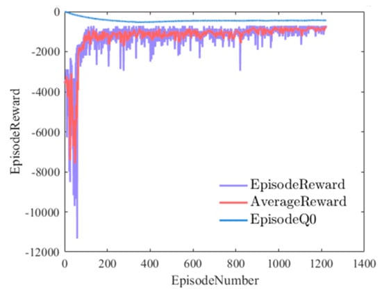
Figure 6.
Episode rewards for mask–wafer leveling with rlDQNAGENTS.
As the training process progressed, the algorithm tended to become stable. Specifically, the episode reward and average reward tended to stabilize. The CNN-Behavior network estimated the Q-value of the action, so Episode Q0 and Episode Reward maintained a certain difference.
As shown in Figure 7, in order to test the stability of the algorithm and its adaptability to different models, a comparative analysis was conducted on the horizontal plane tilt environment model (x–y) and the vertical plane tilt environment model (x–z) from two perspectives: the learning curve and Episode Q0. As shown in Figure 7c, the horizontal plane tilt environment model included the mask and wafer in the horizontal plane, as well as the generated Moiré-based phase imaging. The mask was in a balanced state, while the wafer was in an in-plane tilted state. The tilt angle was 30 degrees. This paper measures angles from 0.1 to 60 degrees in the environmental input and measures them proportionally. The 30 degrees here are just a set of simulation conditions as an example to simulate the leveling accuracy of this strategy in the case of large angles. The alignment mark of the mask was a line grating with a period of 4 μm and a duty cycle of 1:1. The alignment mark period of the wafer was 4.2 μm. A line grating with a duty cycle of 1:1 is generated because the wafer was in the horizontal plane tilted state. This produced the horizontal plane inclined Moiré fringe. As shown in Figure 7d, the vertical plane tilt environment model (x–z) included the mask and wafer in the x–z direction and the generated Moiré-based phase imaging. The mask was in a balanced state, while the wafer was tilted in space. The tilt angle in the z direction was 30 degrees. The mold alignment mark period was 4 µm, and the duty ratio was 1:1 for the line grating. The period of the wafer alignment mark was 4.2 μm, and the line grating duty ratio was 1:1 due to the tilt of the wafer in space, thereby affecting the frequency and angle of the fringes, generating an inclined Moiré fringe in the vertical plane. The thickness of the upper and lower stripes was inconsistent.
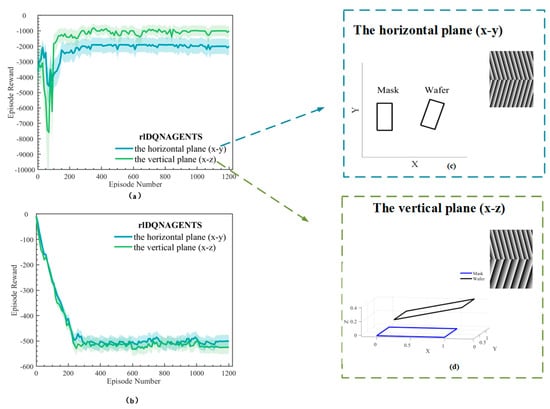
Figure 7.
Comparison between two models in rlDQNAGENTS: (a) learning curve comparison; (b) Episode Q0 comparison; (c) the horizontal plane tilt environment model (x–y); (d) the vertical plane tilt environment model (x–z).
As shown in Figure 7a, the simulation results indicate that in the comparison of the learning curves, the vertical plane tilt environment model (x–z) needed to adjust the angle in the vertical direction. While leveling the angle in the vertical direction, it also needed to level the angle in the x–y direction. Therefore, before iterating 200 times within the time period, the fluctuations and errors were larger than those of the horizontal plane tilt environment model (x–y), and the converged Episode Reward was 200 higher than that of the horizontal plane. As shown in Figure 7b, in the Episode Q0 comparison, the convergence curves of the two models do not differ by much. Therefore, this algorithm has good robustness in terms of model adaptability.
3. Discussion
In order to determine the effectiveness of the algorithm, we analyzed the phase solution of the tilted Moiré fringe generated by the horizontal plane tilt environment model (x–y) and the vertical plane tilt environment model (x–z). During the phase solution process, we drew on the methods of Zhu et al. [9,10] and Zhou et al. [11,12] to solve the tilted Moiré fringe. Zhu et al. [10] used the spatial frequency method to solve the tilted Moiré fringe. For a four-quadrant Moiré fringe, the adjustment accuracy reached rad. The average error and standard deviation in the x–y direction were 0.005308 degrees and 0.004332 degrees, respectively. In the x–z direction, the average error and standard deviation were 0.005308 degrees and 0.004627 degrees [9]. Zhou et al. [11] utilized the tilt modulation spatial phase imaging method to address wafer–mask leveling. The adjustment accuracy of this method reached rad. They improved upon this method and proposed Moiré-based phase imaging for sensing and adjustment [12]. The adjustment accuracy of the in-plane twist angle reached rad.
As shown in Figure 8b,d, the wavelength was 633 nm, and the alignment mark of the mask was a line grating with a period of 4 μm and a duty cycle of 1:1. The alignment mark period of the wafer was 4.2 μm, and different Moiré fringes were generated based on the two directions of the horizontal and vertical plane. According to Formulas (5)–(9), phase analysis was performed on the tilted Moiré fringe, and the phase images of the tilted Moiré fringe generated by the two models were calculated. The simulation results are shown in Figure 8a,c for tilt angles and frequencies in various directions. Figure 8a shows the relationship between the normalized frequency and the tilt angle of the horizontal plane (x–y). The angles in the horizontal plane ranged from −2° to 3°. The theoretical error of the angle deviation after applying the DQN algorithm leveling was 0.0011 degrees. Ten repeated angle deviations were conducted at the same angle after applying the DQN algorithm leveling, and the accuracy of the repeated measurements was 0.00025 degrees. Figure 8c illustrates the relationship between the angular deviation of the vertical plane (x–z) and the angle in the direction of the vertical plane. The angle in the vertical plane ranged from −0.5° to 0.6°. Since the frequency and angle were affected in the vertical plane, the frequency was quite different from the normalized frequency. The theoretical accuracy of the angle deviation after applying the DQN algorithm leveling was 0.0043 degrees. Ten repeated angle deviations were conducted at the same angle after applying the DQN algorithm leveling, and the accuracy of the repeated measurements was 0.00027 degrees. Compared with the vertical plane direction, the angle deviation accuracy in the horizontal plane was lower after DQN leveling. The repeated measurement accuracy did not differ by much. In practical applications, this strategy should be combined with industrial software, and the movement and stop of the in situ grating or photoelectric limit sensor of the workpiece table can be controlled through the setting of industrial software and loss function parameters. Taking a proximity lithography machine as an example, the wafer grating and the mask grating overlap to generate a Moiré fringe image. The moving Moiré fringe is detected by the CCD camera. The image is input to the industrial software containing this strategy, thereby automatically adjusting the movement of the mask and the wafer state, and the setting of the loss function parameters is mainly to ensure that the mask and wafer are in a normal rather than tilted state and should be optimized according to different scenarios.
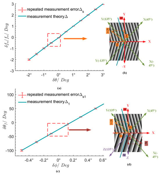
Figure 8.
The normalized frequency and angular deviation of the Moiré fringe tilt relative to (a) the horizontal plane, (b) the vertical plane, (c) the angle calculation of the horizontal plane, and (d) the angle calculation of the vertical plane.
4. Conclusions
This paper describes a proposed mask and wafer leveling strategy based on the Deep Q-Network (DQN) algorithm. The method is based on the mechanism of the DQN algorithm, taking a set of discrete continuous-tilt wafer tilt images as its input. According to the different tilt directions, the models were divided into two groups: the horizontal plane tilt environment model (x–y) and the vertical plane tilt environment model (x–z). A set of four discrete tilt images was input into the CNN-Behavior network in the DQN algorithm for training. After the experience replay pool in the DQN algorithm continuously interacted with the environment, the Q-value representing the best action for each iteration was determined. After continuous iterations, the automatic leveling of masks and wafers was achieved. The tilted Moiré fringes generated by specific tilt angles of the wafer were simulated, and then the Moiré fringes generated in different tilt planes after adjustment via the DQN algorithm were calculated according to the formula and through repeated measurements at the same angle. In the horizontal plane, the accuracy of the x–y angle deviation reached 0.0011 degrees, and the accuracy of repeated angle deviation reached 0.00025 degrees. The accuracy of the angle deviation in the vertical plane (x–z) reached 0.0043 degrees, and the accuracy of repeated angle measurements reached 0.00027 degrees. The research results obtained from leveling strategies meet the directional leveling requirements of the current alignment process for various tilts. In practical applications, the combination of this adjustment strategy and industrial operation software enhances the accuracy of detecting the motion status of the mask and wafer, provided that the reference plane of the mask and wafer is determined. In the future, we will continue to conduct research combining it with actual scenarios to increase the possibility of applying this technology to industry., but it still has some shortcomings. The early model requires a long training time, and the training process needs to be well configured to run.
Author Contributions
Conceptualization, C.J. and J.Z.; writing—original draft preparation, C.J.; writing—review and editing, H.S. and D.Y.; supervision and experimental work, J.L. and J.W. All authors have read and agreed to the published version of the manuscript.
Funding
The work was supported by the grant from the National Key Research and Development Plan (grant number 2021YFB3200204), the Sichuan Provincial Regional Innovation Cooperation Project (2024YFHZ0189), the Sichuan Provincial Science Fund for Distinguished Young Scholars (2024NSFJQ0027), the National Natural Science Foundation of China (grant number 61604154, 61875201, 61975211, 62005287).
Institutional Review Board Statement
Not applicable, as this study did not involve human subjects or animals.
Informed Consent Statement
Not applicable, as this study did not involve human subjects or animals.
Data Availability Statement
The data underlying the results presented in this paper are not publicly available at this time but may be obtained from the authors upon reasonable request.
Conflicts of Interest
The authors declare no conflicts of interest.
References
- Tomonori, D.; Yuji, S.; Takanobu, O.; Hajime, Y.; Yujiro, H.; Brown, J.; Go, I.; Masahiro, M.; Yuichi, S. On-product overlay improvement with an enhanced alignment system. Proc. SPIE 2017, 10147, 343–350. [Google Scholar] [CrossRef]
- Chris, A.M. Fundamental Principles of Optical Lithography; Wiley: Hoboken, NJ, USA, 2007. [Google Scholar] [CrossRef]
- Nianhua, L.; Wei, W.; Stephen, Y.C. Sub-20-nm Alignment in Nanoimprint Lithography Using Moiré Fringe. Nano Lett. 2006, 6, 2626–2629. [Google Scholar] [CrossRef]
- Jae-Hwang, L.; Chang-Hwan, K.; Yong-Sung, K.; Kai-Ming, H.; Kristen, P.C.; Leung, W.Y.; Cheol, O. Diffracted moiré fringes as analysis and alignment tools for multilayer fabrication in soft lithography. Appl. Phys. Lett. 2005, 86, 204101. [Google Scholar] [CrossRef]
- Mühlberger, M.; Bergmair, I.; Schwinger, W.; Gmainer, M.; Schöftner, R.; Glinsner, T.; Hasenfuß, C.; Hingerl, K.; Vogler, M.; Schmidt, H.; et al. A Moiré method for high accuracy alignment in nanoimprint lithography. Microelectron. Eng. 2007, 84, 925–927. [Google Scholar] [CrossRef]
- Jianguo, Z.; Song, H.; Junsheng, Y.; Shaolin, Z.; Yan, T.; Min, Z.; Lei, Z.; Minyong, C.; Lanlan, L.; Yu, H.; et al. Four-quadrant gratings moiré fringe alignment measurement in proximity lithography. Opt. Express 2013, 21, 3463–3473. [Google Scholar] [CrossRef]
- Xu, F.; Zhou, S.; Hu, S.; Jiang, W.; Luo, L.; Chu, H. Moiré fringe alignment using composite circular-line gratings for proximity lithography. Opt. Express 2015, 23, 20905–20915. [Google Scholar] [CrossRef]
- Zhu, J.; Hu, S.; Yu, J.; Tang, Y.; Xu, F.; He, Y.; Zhou, S.; Li, L. Influence of tilt moiré fringe on alignment accuracy in proximity lithography. Opt. Lasers Eng. 2013, 51, 371–381. [Google Scholar] [CrossRef]
- Zhu, J.; Hu, S.; Yu, J.; Tang, Y. Alignment method based on matched dual-grating moiré fringe for proximity lithography. Opt. Eng. 2012, 51, 113603. [Google Scholar] [CrossRef]
- Jiangping, Z.; Song, H.; Xianyu, S.; Zhisheng, Y. Adjustment Strategy for Inclination Moiré Fringes in Lithography by Spatial Frequency Decomposition. IEEE Photonics Technol. Lett. 2015, 27, 395–398. [Google Scholar] [CrossRef]
- Zhou, S.; Yang, Y.; Zhao, L.; Hu, S. Tilt-modulated spatial phase imaging method for wafer-mask leveling in proximity lithography. Opt. Lett. 2010, 35, 3132–3134. [Google Scholar] [CrossRef]
- Zhou, S.; Xie, C.; Yang, Y.; Hu, S.; Xu, X.; Yang, J. Moiré-Based Phase Imaging for Sensing and Adjustment of In-Plane Twist Angle. IEEE Photonics Technol. Lett. 2013, 25, 1847–1850. [Google Scholar] [CrossRef]
- Xing, H.; Gao, Z.; Wang, H.; Lei, Z.; Ma, L.; Qiu, W. Digital rotation moiré method for strain measurement based on high-resolution transmission electron microscope lattice image. Opt. Lasers Eng. 2019, 122, 347–353. [Google Scholar] [CrossRef]
- Wang, N.; Jiang, W.; Zhang, Y. Deep learning–based moiré-fringe alignment with circular gratings for lithography. Opt. Lett. 2021, 46, 1113–1116. [Google Scholar] [CrossRef]
- Wang, N.; Jiang, W.; Zhang, Y. Moiré-based sub-nano misalignment sensing via deep learning for lithography. Opt. Lasers Eng. 2021, 143, 106620. [Google Scholar] [CrossRef]
- Mnih, V.; Kavukcuoglu, K.; Silver, D.; Rusu, A.A.; Veness, J.; Bellemare, M.G.; Graves, A.; Riedmiller, M.; Fidjeland, A.K.; Ostrovski, G.; et al. Human-level control through deep reinforcement learning. Nature 2015, 518, 529–533. [Google Scholar] [CrossRef] [PubMed]
- Devo, A.; Mezzetti, G.; Costante, G.; Fravolini, M.L.; Valigi, P. Towards Generalization in Target-Driven Visual Navigation by Using Deep Reinforcement Learning. IEEE Trans. Robot. 2020, 36, 1546–1561. [Google Scholar] [CrossRef]
- Ngan, L.; Vidhiwar Singh, R.; Kashu, Y.; Khoa, L.; Marios, S. Deep reinforcement learning in computer vision: A comprehensive survey. Artif. Intell. Rev. 2021, 55, 2733–2819. [Google Scholar] [CrossRef]
- Yuling, H.; Xiaoping, L.; Chujin, Z.; Yunlin, S. DADE-DQN: Dual Action and Dual Environment Deep Q-Network for Enhancing Stock Trading Strategy. Mathematics 2023, 11, 3626. [Google Scholar] [CrossRef]
- Fu Hai, Z.; Guangjun, S. Planar Delaunay Mesh Smoothing Method Based on Angle and a Deep Q-Network. Appl. Sci. 2023, 13, 9157. [Google Scholar] [CrossRef]
- Keecheon, K. Multi-Agent Deep Q Network to Enhance the Reinforcement Learning for Delayed Reward System. Appl. Sci. 2022, 12, 3520. [Google Scholar] [CrossRef]
- Zhaoming, W.; Ye-bo, Y.; Jie, L.; De, Z.; Jie, C.; Wei, J. A Novel Path Planning Approach for Mobile Robot in Radioactive Environment Based on Improved Deep Q Network Algorithm. Symmetry 2023, 15, 2048. [Google Scholar] [CrossRef]
Disclaimer/Publisher’s Note: The statements, opinions and data contained in all publications are solely those of the individual author(s) and contributor(s) and not of MDPI and/or the editor(s). MDPI and/or the editor(s) disclaim responsibility for any injury to people or property resulting from any ideas, methods, instructions or products referred to in the content. |
© 2024 by the authors. Licensee MDPI, Basel, Switzerland. This article is an open access article distributed under the terms and conditions of the Creative Commons Attribution (CC BY) license (https://creativecommons.org/licenses/by/4.0/).