Richardson–Lucy Iterative Blind Deconvolution with Gaussian Total Variation Constraints for Space Extended Object Images

Abstract

In ground-based astronomical observations or artificial space target detections, images obtained from a ground-based telescope are severely distorted due to atmospheric turbulence. The distortion can be partially compensated by employing adaptive optics (pre-detection compensation), image restoration techniques (post-detection compensation), or a combination of both (hybrid compensation). This paper focuses on the improvement of the most commonly used practical post-processing techniques, Richardson–Lucy (R–L) iteration blind deconvolution, which is studied in detail and improved as follows: First, the total variation (TV) norm is redefined using the Gaussian gradient magnitude and a set scheme for regularization parameter selection is proposed. Second, the Gaussian TV constraint is proposed to impose to the R–L algorithm. Last, the Gaussian TV R–L (GRL) iterative blind deconvolution method is finally presented, in which the restoration precision is visually increased and the convergence property is considerably improved. The performance of the proposed GRL method is tested by both simulation experiments and observed field data.

1. Introduction

Adaptive optics image restoration [1] is a key post-processing task in ground-based optical imaging of space targets [2]. Among all the restoration methods based on single or multiple frame images including speckle imaging [3], wave-front sensing deconvolution [4,5], blind deconvolution [6,7], and phase difference [8], the blind restoration method is considerably convenient and flexible. In this method, observation source data can be processed independently of telescope equipment; therefore, there has always been a focus on the processing and analysis of space target photoelectric detection data, and this method has successfully been used to carry out image restoration for many large ground-based telescope systems. In some cases, this method can even achieve preferable restoration of target images under strong turbulence conditions [9,10].

In the application field of adaptive optics image restoration, current research on blind deconvolution technology mainly focuses on imposing more effective constraints to improve the convergence property and convergence speed of the algorithm. These works [11,12] are all based on the Bayesian inference framework. At the same time, blind restoration methods have been one of the very important basic research directions in the more general field of natural image processing. In recent years, blind restoration methods for adaptive optics images can be classified into several categories: the Bayesian inference framework [13,14], variational and partial differential equations (VPDE) [15,16], sparse representation [17,18] and deep learning [19,20]. Blind restoration of ground-based optical images for space targets is traditionally based on classic iterative methods derived from noise model statistics under the Bayesian inference framework. Although researchers have carried out preliminary research on adaptive optics image blind restoration methods using VPDE, sparse representation or deep learning techniques, the published literature shows that the restoration effectiveness of these methods was practically demonstrated for field data.

Due to the intractability of the blind recovery problem and the stochastic nature of the imaging scene, blind recovery methods based on Bayesian frameworks, VPDE, sparse representations, or deep learning are not well generalized. The research work in the field of ground-based adaptive optics image blind recovery for both space point and extended targets still focuses on improving the recovery performance by imposing physical constraints in a Bayesian framework. VPDE image processing techniques have achieved significant research progress in recent years, providing good results in the application fields of image restoration, segmentation, reconstruction, recognition and analysis. In particular, image post-processing and analysis techniques based on the total variation (TV) model [21,22] have shown certain advantages in the field of photoelectric imaging detection.

This paper takes the total variation minimization as the improved post-processing framework, and combines the characteristics and demands of ground-based photoelectric detection, then focuses on addressing the deficiencies of the most commonly used blind deconvolution algorithm, the classical Richardson–Lucy (RL) iteration [23,24]. This work conducts research on the definition of the Gaussian total variation norm, the selection of the regularization parameter, and the improvement of the convergence performance of the RL iteration. The rest of this paper is organized as follows: Section 2 describes the definition of the Gaussian total variation norm and the minimization model, and introduces a set scheme for regularization parameter selection. Section 3 presents the proposed Gaussian total variation constrained Richardson–Lucy iterative blind deconvolution algorithm, and gives the flow of algorithm execution. Section 4 demonstrates the performance of our method by simulated experiments, and deconvolution results of three synthetic space targets with typical structures are analyzed. Section 5 draws a conclusion of this work.

2. Gaussian Total Variation Constrained Regularization Methods

2.1. Definition of Gaussian Total Variation Norm

Among the image restoration methods based on VPDE, the TV minimization model proposed by Rudin et al. [25] has attracted most attention due to its good edge-preserving properties, which provide considerable advantages in restoration problems such as denoising, deblurring and patching. The TV parameter of the image $u(x,y)$ is defined as the integral of the gradient magnitude of the image, i.e.,

$$TV\left(u\right)={\displaystyle {\iint }_{{\Omega }_u}|\nabla u|dxdy}={\displaystyle {\iint }_{{\Omega }_u}\sqrt{u_x{ }^2+u_y{ }^2}dxdy}$$

(1)

where ${\Omega }_u$ is the support domain of image $u$, and the gradient of the image is the derivative with respect to the horizontal and vertical direction variables $x,y$, expressed by the gradient operator $\nabla u=\left(\partial u/\partial x,\partial u/\partial y\right)=\left(u_x,u_y\right)$. $|\nabla u|$ denotes the gradient magnitude of an image defined by $|\nabla u|=\sqrt{u_x{ }^2+u_y{ }^2}$.

The diffusion operator of the TV regularization recovery method can control its diffusion only along the tangential direction of the edges. Therefore, the target details can be recovered. However, in flat regions, the diffusion along the orthogonal direction of the gradient is likely to result in false edges. To mitigate this problem, we propose the Gaussian TV norm in this paper. Compared with the TV norm that is defined based on the forward finite difference gradient operators, the Gaussian TV norm defines the gradient of an image based on the Gaussian smooth gradient operators [26] $G_x$ and $G_x$ as follows:

$$G_d=\frac{\partial }{\partial d}g\left(x,y\left|\sigma \right.\right)=-\frac{d}{{\sigma }^2}\frac{1}{2\pi {\sigma }^2}\exp \left(-\frac{x^2+y^2}{2{\sigma }^2}\right)$$

(2)

where $d\in \{x,y\}$ represents the horizontal and vertical directions, and $g\left(x,y\left|\sigma \right.\right)$ is a Gaussian function with scale parameter $\sigma$. After using the Gaussian gradient operator, based on the definition of TV in continuous space, the Gaussian TV (GTV) norm presented in this paper is defined as

$$GTV(o)={\displaystyle \sum _{x,y}\left|{\nabla }_{G}o\right|}={\displaystyle \sum _{x,y}\sqrt{{(G_x\otimes o)}^2+{(G_y\otimes o)}^2}}$$

(3)

where ${\nabla }_G$ denotes the Gaussian gradient, and $o$ is the target image. In this way, the anisotropic diffusion operator (ADO) corresponding to the Gaussian TV norm becomes

$$AD{O}_{GTV}(o)=-\nabla \cdot \left(\frac{{\nabla }_{G}o}{\left|{\nabla }_{G}o\right|}\right)$$

(4)

with its diffusion coefficient $|{\nabla }_{G}o{|}^{-1}$. The use of first-order Gaussian partial derivatives to define the TV norm has two advantages over the finite difference operators: First, the Gaussian smoothed gradient operation can pre-suppress parts of the noise, reducing the possibility of mistakenly treating the noise as image edges in the flat region, whereas the finite difference operators amplify the noise. Second, the gradient magnitude of Gaussian (GMG) $\left|{\nabla }_{G}o\right|$ can remove a large amount of image space redundancy and extract the edge information such as lines and corners more accurately. Consequently, $|{\nabla }_{G}o{|}^{-1}$ can more accurately control the diffusion behavior during the iterative solving process.

2.2. The Gaussian Total Variation Minimization Model

For the space target ground-based adaptive optics imaging model, the real image of the target $o(\mathbf{x})$ becomes a degraded focal plane observation $i(\mathbf{x})$ after the action of the degradation function $h(\mathbf{x})$ and the imaging noise $n(\mathbf{x})$, i.e.,

$$i(\mathbf{x})=(h\otimes o)(\mathbf{x})+n(\mathbf{x})$$

(5)

where $\mathbf{x}=(x,y)$ denotes the space coordinate of the image, $h(\mathbf{x})$ represents the point spread function (PSF), and $\otimes$ is a two-dimensional convolution operation.

The basic idea of the blind recovery algorithm based on the TV method is to transform the ill-posed inverse problem into a well-posed benign problem by adding additional constraints on the target image and the point spread function. The basic framework for its solution is to minimize the energy functional. For the above imaging model, the TV energy functional can be achieved by adding the TV constraints on the target image [21]:

$$J_{TV}\left(o\right)=F\left(h\otimes o\right)+\gamma TV\left(o\right)$$

(6)

where $F(h\otimes o)$ is the data fitting term associated with the noise statistical model, and $\gamma$ is the regularization parameter that is generally referred to as the inverse of the Lagrange multiplier. Considering the commonly used Gaussian noise model as an example, the specific form of the above equation is as follows:

$$J_{TV}\left(o\right)={\displaystyle {\iint }_{\Omega }{\left(h\otimes o-i\right)}^{2}dxdy}+\gamma {\displaystyle {\iint }_{\Omega }|\nabla o|dxdy}$$

(7)

For this expression, the Euler–Lagrange equation for the TV minimization energy functional [21] is

$$h_{-}\otimes \left(h\otimes o-i\right)-\gamma \nabla \cdot \left(\frac{\nabla o}{|\nabla o|}\right)=0$$

(8)

where $\nabla \cdot (s)=div(s)=\partial s/\partial x+\partial s/\partial y$ is the divergence operator. The energy functional of our Gaussian TV blind deconvolution method is obtained by applying the Gaussian TV constraint to the TV minimization model as follows:

$$J_{GTV}\left(o\right)={\displaystyle \sum _{x,y}[{(h\otimes o-i)}^T(h\otimes o-i)]}+\gamma {\displaystyle \sum _{x,y}\sqrt{{(G_x\otimes o)}^2+{(G_y\otimes o)}^2}}$$

(9)

where the superscript $T$ denotes the matrix transposition. So the diffusion equation for the target image evolution under this energy functional is

$$\frac{\partial o}{\partial t}=-h_{-}\otimes \left(h\otimes o-i\right)+\gamma \nabla \cdot \left(\frac{{\nabla }_{G}o}{\left|{\nabla }_{G}o\right|}\right)$$

(10)

where $h_{-}=h(-\mathbf{x})$. This diffusion equation is derived based on the Euler–Lagrange equation for the energy functional of the TV minimization. Further details of this derivation will not be provided here due to some general mathematical treatments.

2.3. Determination of Gaussian Total Variation Regularization Parameters

Based on the previous research progress about the selection of regularization parameters, Gong et al. [27] proposed a systematic model for the construction of TV regularization parameters. It is given as

$$\gamma \left(x,y\right)={\gamma }_0\cdot f\left[\beta \cdot EI\left(x,y\right)\right]$$

(11)

where ${\gamma }_0$ is a preset intensity factor, $f(\cdot )$ is a monotonically decreasing constructor, $\beta$ is a positive constant used for adjusting the intensity of ${\gamma }_0$, and $EI(\cdot )$ is a non-negative edge measure function. It can be gathered that although (11) provides a general model for the selection of the TV regularization parameters, it is still not straightforward to determine ${\gamma }_0$, $f(\cdot )$ and $EI(\cdot )$.

For the regularization parameter selection problem of the TV blind recovery method for space target ground-based optical images, followed by the above combined model of Equation (11), three specific parameter determination strategies are proposed: (1) The value of ${\gamma }_0$ should be gradually reduced during the iterative process in order to avoid the trivial solution as much as possible; (2) an easy-to-handle expression of $f(s)=1/\left(1+s\right)$ is used to ensure that the constructor $f(\cdot )$ is a monotonically decreasing convex function within the $[0, +\infty )$ interval; (3) it is proposed to utilize the second-order Gaussian derivatives, i.e., the Laplacian of Gaussian (LoG) operator, to construct the edge measure function $EI(\cdot )$. The LoG is defined as follows [28]:

$$\begin{array}{l}LoG=\frac{{\partial }^2}{\partial x^2}g(x,y\left|\sigma \right.)+\frac{{\partial }^2}{\partial y^2}g(x,y\left|\sigma \right.)\\ =\frac{x^2+y^2-2{\sigma }^2}{{\sigma }^4}\frac{1}{2\pi {\sigma }^2}\exp \left(-\frac{x^2+y^2}{2{\sigma }^2}\right)\end{array}$$

(12)

In this way, the edge measure function can be expressed as $EI(s)=abs(LoG\otimes s)$, where $abs(\cdot )$ computes the absolute value of the matrix elements to ensure the non-negative property of the edge measure. The LoG operator is proposed for the edge metric computation due to the following reasons: First, LoG filtering can reveal the key structural information at the zero-crossing point of the image, which is widely used in the semantic structure representation of the image. Second, the flat region of the space target ground-based images includes not only the flat region of the target in the general sense, but also the background of the deep space. The values of the parameters within the flat region should be distinguished and, therefore, from the perspective of adaptive selection, the LoG operation should be used to calculate the edge metric function instead of the first-order gradient operator.

Combining the above three selection strategies, the final regularization parameter calculation method is obtained as

$${\gamma }_G\left(x,y\right)=\frac{{\gamma }_0}{1+\beta \cdot abs\left[LoG\otimes o(x,y)\right]}$$

(13)

where ${\gamma }_0$ decreases gradually as the iterations increase, which can be handled in practice by varying it as ${\gamma }_0^{k+1}=0.99{\gamma }_0^k$ or other simple methods.

3. Gaussian Total Variation Constrained Richardson–Lucy Iterative Blind Deconvolution

3.1. Richardson–Lucy Iterative Blind Deconvolution

The Richardson–Lucy iterative blind deconvolution (RL-IBD) method is a synthesis of the iterative blind deconvolution (IBD) algorithm and the non-blind Richardson–Lucy deconvolution algorithm. The spatial and frequency domain expressions of the imaging model given by (5) are rewritten as

$$\left\{\begin{array}{l}i(x,y)=h(x,y)\otimes o(x,y)+n(x,y)\\ I(u,v)=H(u,v)\Theta (u,v)+N(u,v)\end{array}\right.$$

(14)

where $I,H,\Theta ,N$ represent the Fourier space of the observed image, the degraded PSF, the real target image and the noise term, respectively. The principle of the IBD algorithm can be summarized as follows: Starting from the initial estimate ${\widehat{o}}_0$ of the target image, the algorithm iterates alternately in spatial and Fourier frequency domains. Physical constraints are imposed on the target image and the point spread function in the spatial and frequency domains, respectively, until the predefined number of iterations is reached. The principle of the algorithm is based on the maximum likelihood estimation under the Poisson noise model of the image, i.e., the main noise in the image is considered to be photon noise, and the target image is estimated using $\widehat{o}=\arg \max p(i|o)$. The iterative estimation formula can be written [23,24] as follows:

$$o^{k+1}=\left(\frac{i}{h\otimes o^k}\oplus h\right)\cdot o^k$$

(15)

where $\oplus$ denotes the correlation operation, and “$\cdot$” represents dot multiplication. The R–L algorithm has two properties that are useful for image restoration: (1) The R–L iterative process can maintain the non-negativity of the image grayscale, and (2) the sum of the intensity of all the pixels of the image remains unchanged during the iterations.

3.2. Gaussian Total Variation Constrained RL-IBD Blind Deconvolution Algorithm

The execution of the RL-IBD algorithm is based on the IBD framework, which is simple in design and easy to handle. However, the iterative formula derived from the maximum likelihood estimation does not incorporate regularization constraints on the target image. Consequently, the stability and convergence of the algorithm are not guaranteed when dealing with the inverse problem of blind image recovery. It is possible that the recovery results completely consist of amplified noise when the number of iterations is large. On the other hand, the RL-IBD algorithm sharpens the image during its execution process; therefore, the gray value of the edge region increase in the early stage of the iteration. However, since the algorithm ensures that the sum of the gray values of the image remains unchanged, the gray values of the flat region are reduced that cause the image to darken visually. This phenomenon continues over a large number of iterations, meanwhile, the noise is severely amplified for a very high number of iterations.

Therefore, the iterative process should be terminated before the edge regions of the image reach a certain degree of clarity and the noise is amplified. The design of the RL-IBD algorithm does not automatically determine the termination condition. The gray values of the flat regions of the image become smaller during the early and middle stages of the algorithm execution because of the edge sharpening. Thus, it is possible to apply the Gaussian TV constraints proposed in the previous section to the image so that the gradient of the edge regions or the overall gradient of the image do not increase too fast, which makes the image deblurring process smoother. The objective functional of the RL-IBD algorithm after adding the Gaussian TV constraint is defined as:

$$\begin{array}{l}{J}_{GRL}(o):=J_{RL}(o)+J_{GTV}(o)\\ ={\displaystyle \sum _{x,y}\left(-i\log (h\otimes o)+h\otimes o\right)}+{\gamma }_{GRL}{\displaystyle \sum _{x,y}\left|{\nabla }_{G}o\right|}\end{array}$$

(16)

where ${\gamma }_{GRL}$ is the regularization parameter that balances the likelihood and constraint terms. Minimization of (16) using a gradient-based numerical optimization algorithm is equivalent to employing a penalized likelihood expectation maximization algorithm. This requires the computation of the partial derivatives of the objective function with respect to the image and the PSF as follows:

$$\frac{\partial J_{GTV}(o)}{\partial o}=-{\gamma }_{GRL}\nabla \cdot \left(\frac{{\nabla }_{G}o}{\left|{\nabla }_{G}o\right|}\right)$$

(17)

Combining the R–L algorithm with (17) will result in the following expression by searching for the solution of equation $\partial J_{GRL}(o)/\partial o=0$:

$$\left(\frac{i}{h\otimes o^k}\oplus h\right)\cdot \frac{1}{1-{\gamma }_{GRL}\nabla \cdot \left(\frac{{\nabla }_G{o}^k}{\left|{\nabla }_G{o}^k\right|}\right)}=1$$

(18)

where $o^k$ is the image estimation at the kth iteration. Multiplying both ends of the equation simultaneously by $o^k$, and using the Picard iteration principle, the target image iteration formula of the Gaussian TV constrained R–L algorithm can be obtained as:

$$o^{k+1}=\left(\frac{i}{h\otimes o^k}\oplus h\right)\cdot \frac{o^k}{1-{\gamma }_{GRL}\nabla \cdot \left(\frac{{\nabla }_G{o}^k}{\left|{\nabla }_G{o}^k\right|}\right)}$$

(19)

Finally, similar to the treatment of PSF estimation in the RL-IBD algorithm, substituting both the target image and the PSF estimation into the IBD framework, the iterative computational formulation of the Gaussian total variation constrained RL-IBD algorithm (GRL algorithm) proposed in this section is given as follows:

$$\left\{\begin{array}{l}{h}^{k+1}=\left(\frac{i}{h^k\otimes o^k}\oplus o^k\right)\cdot h^k\\ o^{k+1}=\left(\frac{i}{h^{k+1}\otimes o^k}\oplus h^{k+1}\right)\cdot \frac{o^k}{1-{\gamma }_{GRL}\nabla \cdot \left(\frac{{\nabla }_G{o}^k}{\left|{\nabla }_G{o}^k\right|}\right)}\end{array}\right.$$

(20)

The regularization parameter ${\gamma }_{GRL}$ is selected according to the strategy proposed in the previous section. To maintain the computational efficiency, the correlation as well as convolution operations involved in the GRL algorithm proposed in this section are realized in the Fourier domain. The final hybrid iterative formula corresponding to the above equation is:

$$\left\{\begin{array}{l}{h}^{k+1}=h^k{\mathcal{F}}^{-1}\left[{\Theta }_k^{\ast }\mathcal{F}\left(\frac{i}{{\mathcal{F}}^{-1}\left(H_k{\Theta }_k\right)}\right)\right]\\ o^{k+1}=\frac{o^k}{1-{\gamma }_{GRL}\nabla \cdot \left(\frac{{\nabla }_G{o}^k}{\left|{\nabla }_G{o}^k\right|}\right)}{\mathcal{F}}^{-1}\left[H_{k+1}^{\ast }\mathcal{F}\left(\frac{i}{{\mathcal{F}}^{-1}\left(H_{k+1}{\Theta }_k\right)}\right)\right]\end{array}\right.$$

(21)

where $\mathcal{F}$ and ${\mathcal{F}}^{-1}$ represent the Fourier transform and its inverse transform, respectively, ${\Theta }^{*}$ and $H^{*}$ represent the complex conjugate of $\Theta$ and $H$, respectively. The algorithm is terminated when the number of outer iterations reaches a predefined limit or the relative error of the successive estimations (RESE) between two neighboring iterations is less than a predefined value. The selection of the initial value of the target image and the point spread function is similar to the selection of the initial value of the RL-IBD algorithm.

The key feature of the GRL iterative blind deconvolution algorithm is that the Gaussian TV norm constraints are imposed during the iterations over the target image. Compared with the existing regularization recovery methods based on VPDE, the algorithm’s computational complexity is significantly less. However, a larger number of iterations are needed for convergence, which is attribute to that the GRL iterative blind deconvolution algorithm is still based on the simple IBD framework. At the same time, compared with the classical RL-IBD algorithm, the maximum penalized likelihood estimation makes the deblurring process smoother by adding effective regularization constraints. This sharpens the edges of the image without excessively suppressing the grayscale values of the smoothed regions. Algorithm 1 shows the execution steps of the entire GRL iterative blind deconvolution algorithm, where the superscripts of the image $o$ and PSF $h$ represent the inner iteration, and the subscripts represent the outer iteration.

Algorithm 1. GRL iterative blind deconvolution algorithm

Initialization: $h_0, {\gamma }_{GRL}^0, K, E_{\infty }, A{F}_o^0, A{F}_h^0, k=0$

Input: $i\to o_0$

While $k\le K$ do

$m=1$; $A{F}_h=A{F}_h^0$; $h^1=h_k$;

For $m\le A{F}_h$

$h^{m+1}=H_{GRL}(h^m, o_k)$; $A{F}_h=A{F}_{GRL}(h^{m+1}, o_k, E_{\infty })$; $m=m+1$;

End

$h_{k+1}=h^{m+1}$; $n=1$; $A{F}_o=A{F}_o^0$; $o^1=o_k$;

For $n\le A{F}_o$

${\gamma }_{GRL}^n={\gamma }_{GRL}({\gamma }_{GRL}^0, o^n)$; $o^{n+1}=O_{GRL}(o^n, h_{k+1}, {\gamma }_{GRL}^n)$;

$A{F}_o=A{F}_{GRL}(h_{k+1}, o^{n+1}, E_{\infty })$; $n=n+1$;

End

$o_{k+1}=o^{n+1}$; $k=k+1$;

End

Output: $\widehat{o}=o_{k+1}; \widehat{h}=h_{k+1}$

The above $A{F}_o^0, A{F}_h^0$ denote the asymmetric factors [29] of estimated image and PSF, respectively. $E_{\infty }$ is an empirical guess of the energy ratio between actual PSF and sharp target image. The idea of asymmetric iteration from Biggs [29] is also adopted in our method, since the number of inner iteration for PSF is a little bigger than that for the estimated image at the beginning of iteration. The flow chart of our proposed GRL deconvolution algorithm is illustrated by Figure 1.

4. Simulation Results and Analysis

The recovery results of space target optical images are evaluated through the accuracy and stability of the presented algorithms. In this section, the performance of the GRL iterative blind deconvolution algorithm will be tested against the RL-IBD algorithm via simulation experiments. The atmospheric turbulence degraded images are simulated based on the Zernike polynomials and Kolmogorov Spectra inversion methods [30,31]. The short exposure imaging was set to adjust the frozen flow hypothesis, and the adaptive optics was also used for tip/tilt compensation in simulation, more high-order aberrations were not corrected in simulated images. The random Gaussian and Poisson noise with 5~40 dB noise intensity were simultaneously added to the observed images. The recovery accuracy is verified by the commonly used Normalized mean squared error (NMSE) metric, which is defined as $NMSE(k)=\left|\right|{\widehat{o}}_k-o_{dl}|{|}^2/\left|\right|o_{dl}|{|}^2$ with ${\widehat{o}}_k$ is the deconvolution output of the kth iteration, and $o_{dl}$ denotes the diffraction limited image. The stability of the iterative deconvolution process is verified by ERDB (Energy ratio of de-blurred and blurred image) metric with the expression [32,33] of

$$ERDB\left(k\right)=\frac{{\displaystyle \sum {\widehat{o}}_k{ }^2}}{{\displaystyle \sum i^2}}$$

(22)

where $i$ is the observed single frame blurred input. The ERDB metric can measure the fluctuation of image total energy during the iteration.

Three simulation images with typical space target structures are selected for the experiments: The first one (T1) has an obvious antenna structure, the second one (T2) has distinct solar panel structures and the third one (T3) has the characteristics of a space vehicle. The diffraction limited images with a 1.2 m-diameter telescope of the three targets are shown in Figure 2.

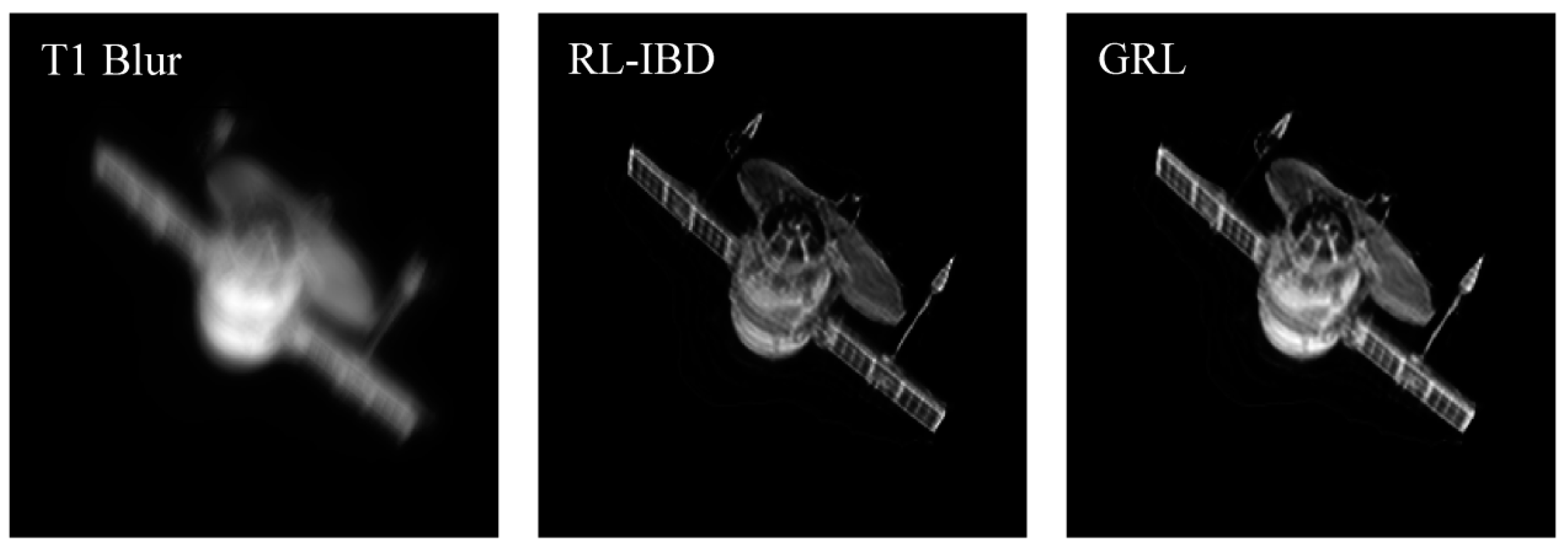
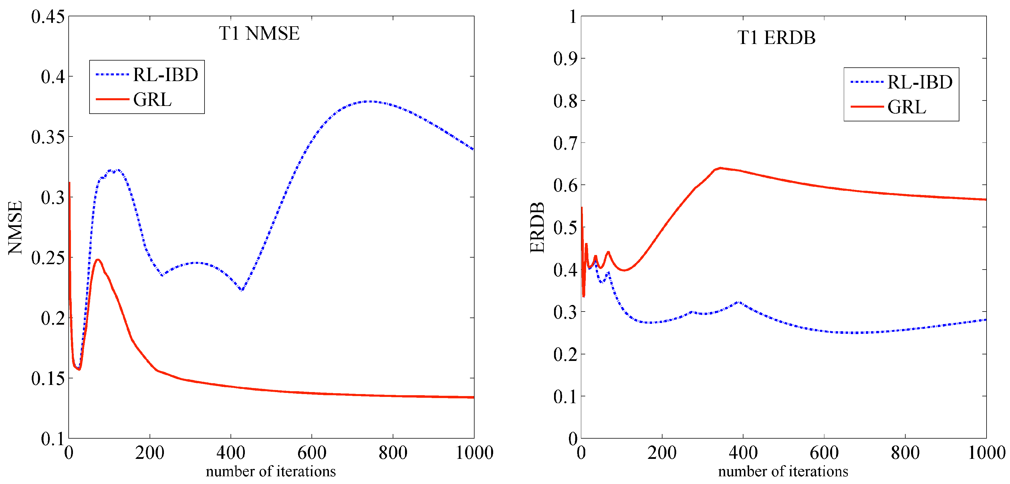
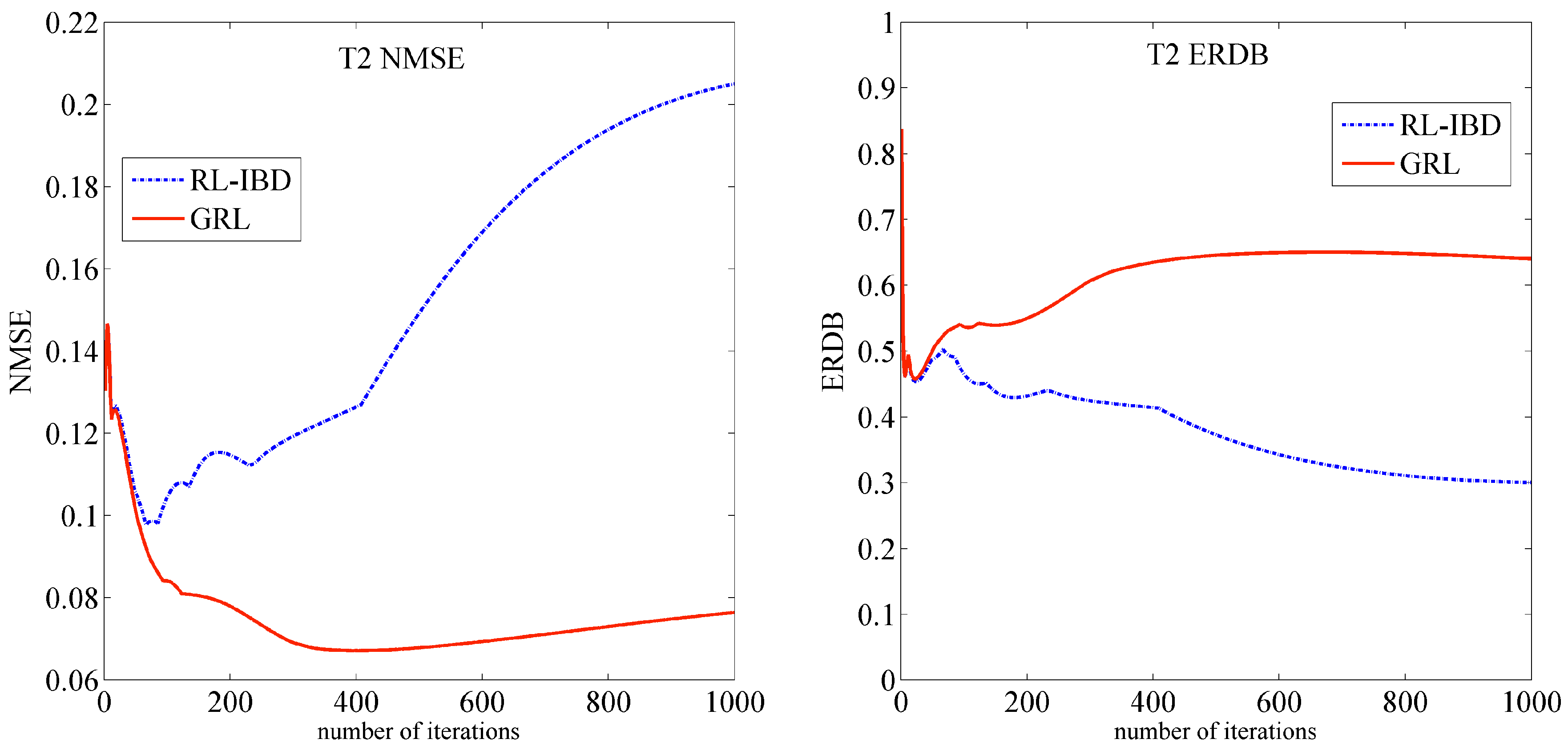
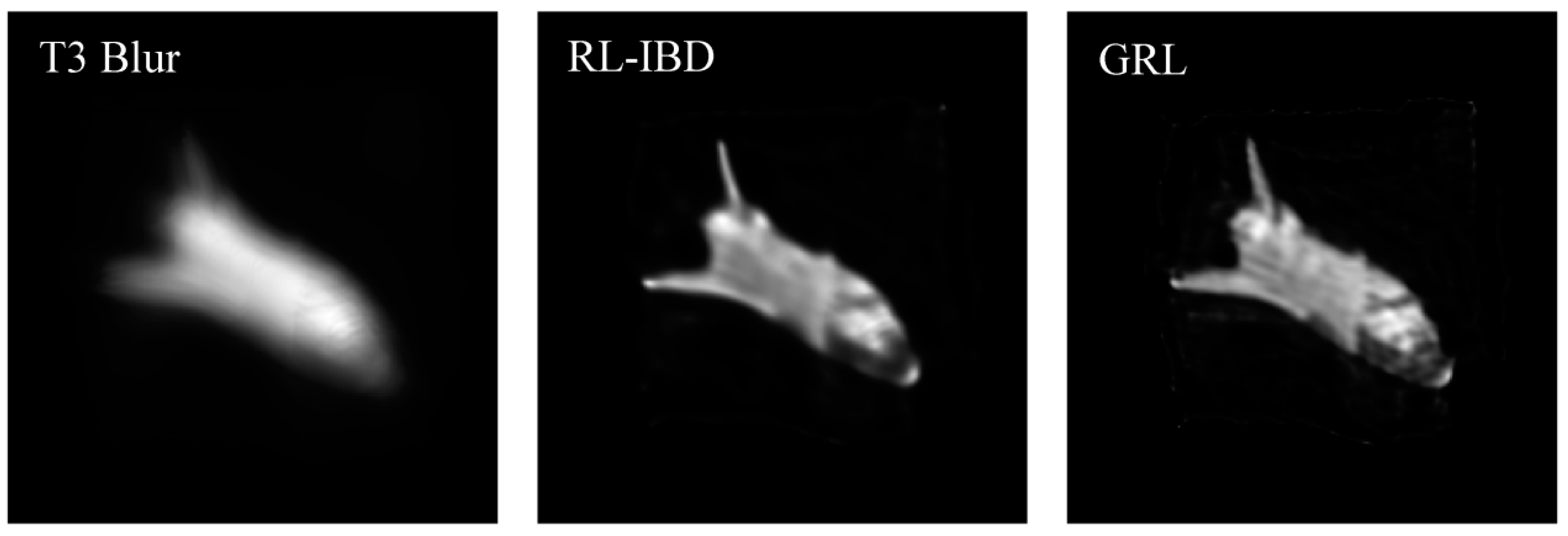
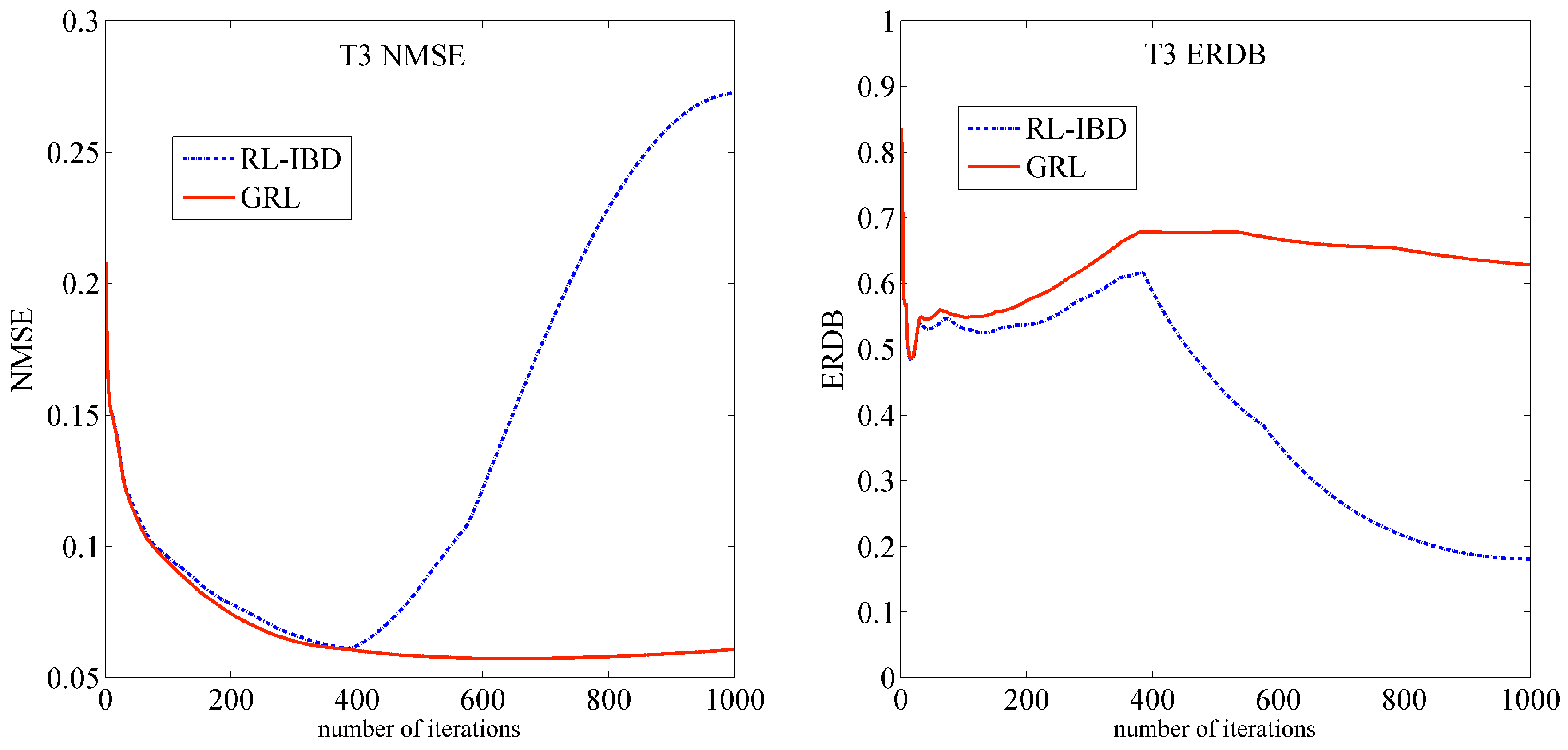
Figure 3, Figure 4, Figure 5, Figure 6, Figure 7 and Figure 8 compare the recovery results of the simulation targets T1, T2 and T3, as well as the NMSE and ERDB results versus the number of iterations. The turbulence intensities used to simulate the blur in T1, T2 and T3 images are $D/r_0=10, 8, 15$, respectively. The initial value of the regularization parameter is set to 0.05 for the GRL algorithm and the results are shown up to 1000 iterations. The time taken in minutes for the recovery of the three images is as follows: T1 [1.9535, 2.2097], T2 [2.4604, 2.6439], and T3 [1.1041, 1.3158], where the first entry in parentheses is the time consumption of the RL- IBD algorithm, and the second entry is that of the GRL algorithm. The computing environments used Windows 7+MATLAB 7.12, Intel i7 2.8 GHz CPU and 16 GB RAM.

From the visual point of view, the recovery results of the GRL algorithm are more detailed compared with the RL-IBD results, referring to the diffraction limited images. The edge shapes of the T1 target antenna and body, the detailed textures of solar panel and connecting units of the T2 target, as well as the tail region shape and structure of the T3 target are more accurately recovered.

The RL-IBD recovery framework combined with the Gaussian TV constraint presents more refined results by subjective assessment. It can be said that the Gaussian total variation constraint brings visual improvement of the recovery results, especially for the target edge region. Meanwhile, the time consumption of the algorithm after imposing the Gaussian TV constraint only increases by about 10% compared with the RL-IBD algorithm.

The NMSE and ERDB results of the three targets show that the RL-IBD deconvolution algorithm is always non-convergent. It sharpens the image after a certain number of iterations while continuously amplifying the noise. However, our GRL algorithm proposed in this work can guarantee the basic convergence property of the deconvolution process, and the experimental results show that it exhibits significantly improvement of convergence behavior. For moderate atmospheric turbulence intensity, i.e., a $D/r_0$ value of around 12, the GRL algorithm can ensure that the deconvolution output results become steady after approximately 400 iterations.

The NMSE values between the iterative outputs and the diffraction-limited images in the experiments are maintained below 0.08, and the ERDB values no longer fluctuate with increasing iterations. This behavior indicates that the gradient of the edge region increases while the overall image energy does not decrease considerably during the deconvolution process. However, the RL-IBD algorithm starts to become unstable after approximately 400 iterations at medium turbulence intensity, which is primarily attributed to that the unconstrained sharpening of the edge regions severely suppresses the gray intensity values of the flat regions in the image as the iteration going on. The image energy continuously decreases within a certain period, which can also be observed from the restoration results of the T1 and T2 targets in Figure 3 and Figure 5, respectively. It seems that the recovery results obtained by RL-IBD algorithm are visually darker than our GRL algorithm.

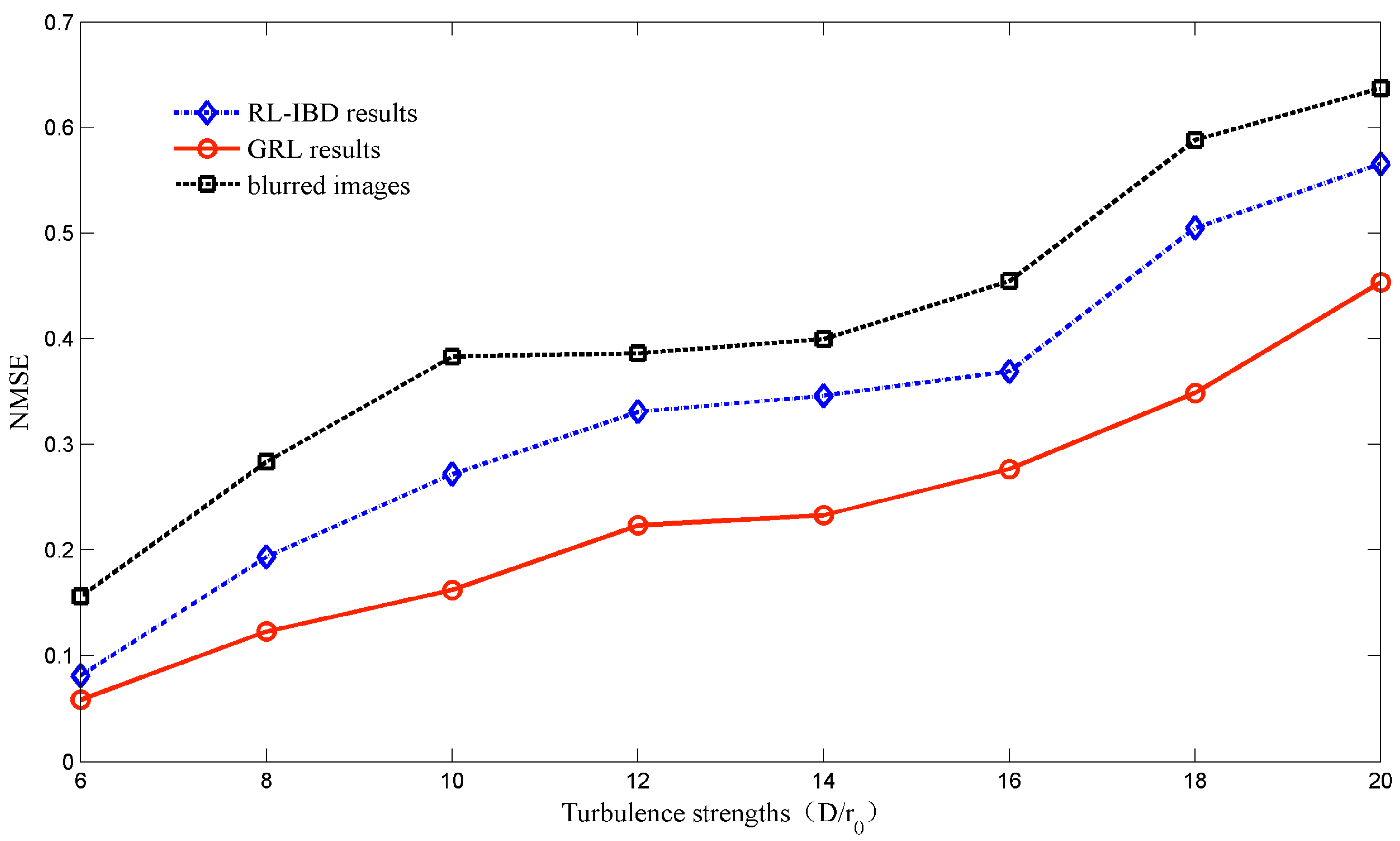
Further, the performance of the post-processing methods under different atmospheric turbulence intensities should also be considered. Figure 9 shows the recovery results obtained using the GRL and RL-IBD algorithms with different turbulence strengths. Note that the RL-IBD algorithm selects the outputs before the noise is amplified. An obvious improvement of the image sharpness can be seen from the NMSE values by our GRL algorithm under different turbulence conditions. This improvement occurs due to the addition of the Gaussian TV constraints. It can be noted from the figure that the GRL algorithm performs better accuracy for recovering degraded images with weak and moderate turbulence intensity from $D/r_0=6$ to $D/r_0=20$.

5. Conclusions and Discussion

This paper proposed an improved Richardson–Lucy iterative blind deconvolution algorithm for ground-based space targets adaptive optics images restoration. The main contributions of this work are as follows: First, a Gaussian gradient-based TV norm was defined, and a set of regularization parameter selection strategies was presented. This was subsequently used to propose a Gaussian TV regularized blind deconvolution algorithm. Second, we proposed to incorporate Gaussian TV constraints into the original RL-IBD algorithm, and then resulting in the Gaussian TV constrained RL-IBD blind recovery method.

The TV regularization method has high recovery accuracy and is theoretically convergent; however, it is computationally intensive and requires a large amount of time to reach the steady-state solution. On the other hand, the RL-IBD method has a simple design and is easy to deal with, but its recovery process is unstable and requires human intervention. The proposed algorithm combined the respective advantages of these methods to overcome their shortcomings. We verified the performance of our proposed algorithm by three sets of simulation experiments. It was experimentally verified to be effective in terms of accuracy, stability, and computational efficiency, and could recover qualified images degraded under less than moderate turbulence strengths. For image recovery with strong turbulence conditions, wave-front measurement data can be derived for estimating high-precision a priori information of the point spread function before deconvolution, which would be the future research work.

References

1. Hampson, K.M.; Turcotte, R.; Miller, D.T.; Kurokawa, K.; Males, J.R.; Ji, N.; Booth, M.J. Adaptive optics for high-resolution imaging. Nat. Rev. Methods Primers 2021, 1, 68. [Google Scholar] [CrossRef] [PubMed]
2. Sturdevant, R.W. From satellite tracking to space situational awareness: The USAF and space surveillance, 1957–2007. Air Power Hist. 2008, 55, 4–23. [Google Scholar]
3. Zhong, L.; Tian, Y.; Rao, C. Speckle image reconstruction of the adaptive optics solar images. Opt. Express 2014, 22, 29249–29259. [Google Scholar] [CrossRef] [PubMed]
4. Jefferies, S.M.; Hart, M. Deconvolution from wave front sensing using the frozen flow hypothesis. Opt. Express 2011, 19, 1975–1984. [Google Scholar] [CrossRef] [PubMed]
5. Guo, S.; Zhang, R.; Li, J.; Zou, J.; Xu, R.; Liu, C. Sequential deconvolution from wave-front sensing using bivariate simplex splines. Opt. Commun. 2015, 342, 73–78. [Google Scholar] [CrossRef]
6. Ayers, G.R.; Dainty, J.C. Iterative blind deconvolution method and its applications. Opt. Lett. 1988, 13, 547–549. [Google Scholar] [CrossRef] [PubMed]
7. Jefferies, S.M.; Christou, J.C. Restoration of astronomical images by iterative blind deconvolution. Astrophys. J. 1993, 415, 862. [Google Scholar] [CrossRef]
8. Gonsalves, R.A. Phase retrieval and diversity in adaptive optics. Opt. Eng. 1982, 21, 829–832. [Google Scholar] [CrossRef]
9. Hart, M.; Jefferies, S.; Hope, D.; Hege, E.K.; Briguglio, R.; Pinna, E.; Puglisi, A.; Quiros, F.; Xompero, M. Multiframe blind deconvolution for imaging in daylight and strong turbulence conditions. In Unconventional Imaging, Wavefront Sensing, and Adaptive Coded Aperture Imaging and Non-Imaging Sensor Systems; SPIE: San Diego, CA, USA, 2011; Volume 8165, pp. 113–118. [Google Scholar]
10. Zhu, X.; Milanfar, P. Removing atmospheric turbulence via space-invariant deconvolution. IEEE Trans. Pattern Anal. Mach. Intell. 2012, 35, 157–170. [Google Scholar] [CrossRef]
11. Babacan, S.D.; Wang, J.; Molina, R.; Katsaggelos, A.K. Bayesian blind deconvolution from differently exposed image pairs. IEEE Trans. Image Process. 2010, 19, 2874–2888. [Google Scholar] [CrossRef]
12. Lee, G.K.; Gelfand, S.B.; Fitz, M.P. Bayesian techniques for blind deconvolution. IEEE Trans. Commun. 1996, 44, 826–835. [Google Scholar]
13. Ruiz, P.; Zhou, X.; Mateos, J.; Molina, R.; Katsaggelos, A.K. Variational Bayesian blind image deconvolution: A review. Digit. Signal Process. 2015, 47, 116–127. [Google Scholar] [CrossRef]
14. Fétick, R.J.-L.; Mugnier, L.M.; Fusco, T.; Neichel, B. Blind deconvolution in astronomy with adaptive optics: The parametric marginal approach. Mon. Not. R. Astron. Soc. 2020, 496, 4209–4220. [Google Scholar] [CrossRef]
15. Perrone, D.; Favaro, P. Total variation blind deconvolution: The devil is in the details. In Proceedings of the IEEE Conference on Computer Vision and Pattern Recognition, Mandi, India, 16–19 December 2014; pp. 2909–2916. [Google Scholar]
16. Molina, R.; Mateos, J.; Katsaggelos, A.K. Blind deconvolution using a variational approach to parameter, image, and blur estimation. IEEE Trans. Image Process. 2006, 15, 3715–3727. [Google Scholar] [CrossRef] [PubMed]
17. Ma, L.; Zhang, R.; Qu, Z.; Lu, F.; Xu, R. Blind image deconvolution using sparse and redundant representation. Optik 2014, 125, 6942–6945. [Google Scholar] [CrossRef]
18. Dong, W.; Wang, Q.; Tao, S.; Tian, C. Blind multi-Poissonian image deconvolution with sparse log-step gradient prior. Opt. Express 2024, 32, 9061–9080. [Google Scholar] [CrossRef] [PubMed]
19. Qiao, C.; Chen, H.; Wang, R.; Jiang, T.; Wang, Y.; Li, D. Deep learning-based optical aberration estimation enables offline digital adaptive optics and super-resolution imaging. Photonics Res. 2024, 12, 474–484. [Google Scholar] [CrossRef]
20. Shi, J.; Zhang, R.; Guo, S.; Yang, Y.; Xu, R.; Niu, W.; Li, J. Space targets adaptive optics images blind restoration by convolutional neural network. Opt. Eng. 2019, 58, 093102. [Google Scholar] [CrossRef]
21. Chan, T.F.; Wong, C.K. Total variation blind deconvolution. IEEE Trans. Image Process. 1998, 7, 370–375. [Google Scholar] [CrossRef]
22. Shao, W.-Z.; Deng, H.-S.; Luo, W.-W.; Li, J.-Y.; Liu, M.-L. Revisiting reweighted graph total variation blind deconvolution and beyond. Vis. Comput. 2023, 40, 3119–3135. [Google Scholar] [CrossRef]
23. Richardson, W.H. Bayesian-based iterative method of image restoration. J. Opt. Soc. Am. 1972, 62, 55–59. [Google Scholar] [CrossRef]
24. Lucy, L.B. An iterative technique for the rectification of observed distributions. Astron. J. 1974, 79, 745. [Google Scholar] [CrossRef]
25. Rudin, L.I.; Osher, S.; Fatemi, E. Nonlinear total variation based noise removal algorithms. Phys. D Nonlinear Phenom. 1992, 60, 259–268. [Google Scholar] [CrossRef]
26. Lin, W.; Kuo, C.C.J. Perceptual visual quality metrics: A survey. J. Vis. Commun. Image Represent. 2011, 22, 297–312. [Google Scholar] [CrossRef]
27. Gong, G.; Zhang, H.; Yao, M. Construction model for total variation regularization parameter. Opt. Express 2014, 22, 10500–10508. [Google Scholar] [CrossRef] [PubMed]
28. Guo, S.; Zhang, R.; Yang, Y.; Xu, R.; Liu, C.; Li, J. Quality metric in matched Laplacian of Gaussian response domain for blind adaptive optics image deconvolution. Opt. Eng. 2016, 55, 043108. [Google Scholar] [CrossRef]
29. Biggs, D.S.C.; Andrews, M. Asymmetric iterative blind deconvolution of multiframe images. In Advanced Signal Processing Algorithms, Architectures, and Implementations VIII; SPIE: San Diego, CA, United States, 1998; Volume 3461, pp. 328–338. [Google Scholar]
30. Galaktionov, I.; Sheldakova, J.; Samarkin, V.; Toporovsky, V.; Kudryashov, A. Atmospheric Turbulence with Kolmogorov Spectra: Software Simulation, Real-Time Reconstruction and Compensation by Means of Adaptive Optical System with Bimorph and Stacked-Actuator Deformable Mirrors. Photonics 2023, 10, 1147. [Google Scholar] [CrossRef]
31. Galaktionov, I.; Sheldakova, J.; Toporovsky, V.; Kudryashov, A. Atmospheric turbulence generator: Software and hardware implementation of Kolmogorov phase screen simulation system. In Laser Resonators, Microresonators, and Beam Control XXVI; SPIE: San Francisco, CA, USA, 2024; Volume 12871, pp. 112–119. [Google Scholar]
32. Ferzli, R.; Karam, L.J. A no-reference objective image sharpness metric based on the notion of just noticeable blur (JNB). IEEE Trans. Image Process. 2009, 18, 717–728. [Google Scholar] [CrossRef]
33. Muller, R.A.; Buffington, A. Real-time correction of atmospherically degraded telescope images through image sharpening. J. Opt. Soc. Am. 1974, 64, 1200–1210. [Google Scholar] [CrossRef]
Figure 1. Flow chart of the proposed GRL deconvolution algorithm.
Photonics 11 00576 g001
Figure 2. Simulation of three typical space target diffraction limited images.
Photonics 11 00576 g002
Figure 3. Comparison of simulated T1 target recovery results.
Photonics 11 00576 g003
Figure 4. T1 target recovery results in terms of NMSE and ERDB.
Photonics 11 00576 g004
Figure 5. Comparison of simulated T2 target recovery results.
Photonics 11 00576 g005
Figure 6. T2 target recovery results in terms of NMSE and ERDB.
Photonics 11 00576 g006
Figure 7. Comparison of simulated T3 target recovery results.
Photonics 11 00576 g007
Figure 8. T3 target recovery results in terms of NMSE and ERDB.
Photonics 11 00576 g008
Figure 9. Accuracy comparison of two algorithms for target T1 image restoration versus varying turbulence strengths.
Photonics 11 00576 g009
Disclaimer/Publisher’s Note: The statements, opinions and data contained in all publications are solely those of the individual author(s) and contributor(s) and not of MDPI and/or the editor(s). MDPI and/or the editor(s) disclaim responsibility for any injury to people or property resulting from any ideas, methods, instructions or products referred to in the content.