Article

Generalized-Mode Averaging Technique for Wrapped Phase

1
National Key Laboratory of Optical Field Manipulaion Science and Technology, Chinese Academy of Sciences, Chengdu 610209, China
2
Institute of Optics and Electronics, Chinese Academy of Sciences, Chengdu 610209, China
3
University of Chinese Academy of Sciences, Beijing 100049, China
4
The Youth Creative Promotion Association, Chinese Academy of Sciences, Beijing 100864, China
*
Authors to whom correspondence should be addressed.
Photonics 2024, 11(6), 561; https://doi.org/10.3390/photonics11060561
Submission received: 25 April 2024 / Revised: 26 May 2024 / Accepted: 3 June 2024 / Published: 14 June 2024

Abstract

:
In this paper, a generalized-mode phase averaging technique is proposed to suppress air turbulence and random noise in optical shop testing. This approach eliminates the need to repeatedly unwrap and thus greatly improves processing efficiency. By removing the random tilt component of the wrapped phase, a set of wrapped phases that are corrupted by random vibrations can be unified into the same mode, some of which obey a circular distribution. Therefore, the circular mean technique can be used for wrapped phase averaging; only one unwrapping process is required for a set of wrapped phases. A criterion based on maximum likelihood estimation is proposed to determine scenarios for the use of this method. The effects of noise and air disturbances on this method are discussed. Finally, the effectiveness of the method is demonstrated by simulations and experiments.

1. Introduction

High-precision, large-diameter optics are widely used in a variety of scenarios and play an irreplaceable role. For example, the ELT telescope and the OWL of the LAMA program have primary mirrors with apertures of 39 m and 100 m, respectively [1].
The precise measurement of figure errors in large-diameter optical elements directly affects their manufacturing accuracy. However, the interferometric cavities of large-diameter components can be tens or even hundreds of meters long. In such a long testing optical path, environmental factors such as vibration and atmospheric turbulence are difficult to control, so how to carry out precision measurements of large-diameter components in a workshop environment has been a research hot spot.
The phase recovery of single-frame interferograms is immune to environmental perturbations; the Fourier method [2], spatial phase shifting [3], and spatial-carrier phase shifting [4] enable transient measurements. However, none of these methods can completely remove the effect of random noise from one or several measurements.
According to classical measurement theory, random noise can be suppressed by simply averaging the data from hundreds or thousands of measurements [5,6]. While this is feasible in the absence of phase jumps, a simple application of this method in the presence of phase wrapping will result in errors. In order to perform averaging, each phase needs to be unwrapped. On the one hand, random noise can be removed, but the time cost is greatly increased. The extension of the measurement period goes against the real-time requirements in industrial measurements. On the other hand, the deformation introduced by the support mechanism during long measurements will also affect the average results. Removal of random noise by only one wrapped phase has also been studied by many scholars. Various filters are used in this scenario [7]: sliding average filters, Gaussian filters, median filters, etc., can all be used in phase demodulation. Later, Qian used the windowed Fourier transform to demodulate the phase, which significantly reduced the effect of random noise [8,9]. Jiang designed an adaptive filter to estimate the orientation and curvature of the pattern to improve detection accuracy [10]. The use of deep learning for denoising has been a hot research topic in recent years, and a number of learning models have been proposed to address the limitations of traditional methods [11]. Meanwhile, in synthetic sub-aperture radars, the related theory of the von Mises distribution is used to measure the correlation of the spatial distribution between the Master and Slave interferograms, which effectively suppresses random noise in the process of minimizing the weighted circular variance. Later, Kim et al. proposed, based on previous geometric unwrapping [12], that random noise can be removed by circular averaging as long as the wrapped phases satisfy the von Mises distribution. Additionally, when processing the wrapped phase in an interferogram, self-mixing interferometry is a good option, as the interferometric fringe is in a distorted sinusoidal pattern [13,14,15]. For random noise, regardless of whether it conforms to a uniform or Gaussian distribution, its mean is 0. Theoretically, by arithmetically averaging the results a sufficient number of times, random noise can then be suppressed. A circular mean or angular mean is a mean designed for angles and similar cyclic quantities, such as times of the day and fractional parts of real numbers. This is necessary since most of the usual means may not be appropriate for angle-like quantities. For example, the arithmetic mean of 0° and 360° is 180°, which is misleading because 360° equals 0° modulo a full cycle. Wrapped phases fit this profile, so using circular averaging for wrapped phases is a more appropriate approach than arithmetic averaging. The advantage of this is that it is no longer necessary to unwrap each wrapped phase, thus saving time. However, the effect of environmental vibrations makes the distributional mode of wrapped phases vary greatly, which generally cannot be averaged directly [16]. Ohgan proposes to cluster the wrapped phase in order to split the data that do not satisfy the conditions of the circular distribution into multiple sets that do satisfy these conditions [17]. This method, which constructs data by similarity, reduces the number of unwrapping procedures to just a few.
However, this approach will still consume a lot of computation and memory resources. In the work of Ohgan et al., the similarity criterion is constructed from the distance between two neighboring wrapped phases. Hundreds of results will typically be captured, and each image can have a resolution of 1024 × 1024 or more, which is a huge drain on time and memory. We still hope that less expensive methods can be devised to realize the removal of random noise. In this paper, we propose a generalized-mode averaging technique to achieve circular averaging, which is more capable of greatly saving time consumption and memory overhead compared to clustering-based methods.

2. Principles

2.1. Von Mises (Circular Normal) Distribution

The von Mises distribution (also known as the circular normal distribution or the Tikhonov distribution) is a continuous probability distribution on a circle. It is an approximation of the encircling normal distribution, which is a circular analog of the normal distribution [18]. The free diffusion angle, θ, on a circle is a wrapped, normally distributed random variable whose unfolded variance grows linearly with time. The von Mises distribution is the maximum entropy distribution of circular data when the real and imaginary parts of the first circular moment are specified. The von Mises distribution is a special case of the von Mises–Fisher distribution on an N-dimensional sphere [19]. The probability density function of the von Mises–Fisher distribution for a random p-dimensional unit vector x is given by
f x , μ , κ = C p κ exp κ μ T x
C p κ = κ p 2 1 2 π p 2 I p / 2 1 κ
If p = 2, the distribution degenerates to the von Mises distribution. Figure 1 shows the situation at p = 2 and p = 3; by the way, the case at p = 3 is also known as the Fisher distribution. The probability density function (PDF) of the von Mises distribution for angle x is given by the following equation:
f x , μ , κ = e κ cos x μ 2 π I 0 κ

2.2. Generalized-Mode Averaging Technique

For the wrapped phase, ψ i ( x , y ) , where the subscript i denotes that it is the result of the i th measurement and ( x , y ) denotes its spatial distribution location, the point can be mapped to a unit circle by the following equation:
X i x , y = cos ψ i x , y , Y i x , y = sin ψ i x , y
If the phasic distribution at this location is highly concentrated and obeys the circular normal distribution well, the random noise can be removed by circular averaging [20]. The result can be obtained by taking its mean value through Equation (5).
ψ ¯ x , y = a r c t a n 2 1 k i = 1 k Y i x , y , 1 k i = 1 k X i x , y
Unfortunately, unprocessed wrapped phases do not naturally obey a circular distribution due to the environment. Ohgan et al. addressed this problem by means of clustering [17]. Although wrapped phases do not satisfy the circular averaging condition when considered over the entire time period, they may satisfy the von Mises distribution separately within groups if all the data are grouped. Classification can be carried out based on the similarity of image modes. It still needs to be unwrapped multiple times. Each grouping requires one instance of unwrapping, which still introduces temporal redundancy.
In this section, a generalized-mode phase averaging technique (GMAT) will be proposed, which not only reduces the number of unwrappings but also reduces memory usage.
An interferogram with an introduced carrier can be represented by Equation (6):
I i x , y = a x , y + b x , y cos f x i x + f y i y + φ x , y + A i r i x , y
where a ,   b ,   φ ,   f x ,   a n d   f y denote the background, modulation, phase, and carrier in the x and y directions, respectively, and Air denotes the phase change due to atmospheric turbulence. The phase obtained by the phase resolution algorithm will be wrapped in p i , p i , as shown in Equation (7).
ϕ i ¯ = W R A P P ( f x i x + f y i y + φ + A i r i )
where W R A P P denotes the wrapping operation, and the subscript i indicates that the current data belong to the ith measurement. Ideally, φ is a function of the spatial position only. f x i , f y i ,   a n d   A i r i are not only location-dependent but also time-dependent. These three variables directly affect the distribution of ϕ i ¯ . Figure 2 shows the wrapped phases of the different modes, and it is actually quite intuitive to see that a direct averaging of these images is forbidden. And on a statistical level, such data will never satisfy a circular distribution.
A few assumptions are first made here based on experience with practical measurements. The effect of vibrations is of a low order; specifically, the vibration introduces a tilt to the phase and only affects f x i   a n d   f y i [21]. The vibration is very rapid in terms of change and may be very different from frame to frame. In contrast, the aberration introduced by atmospheric turbulence is of a relatively high order and is slow-varying compared to the vibration. Second, the aberration analysis shows that the vibration is the main factor affecting the mode, while atmospheric turbulence has a secondary influence. The above assumptions can be summarized by Equation (8).
f x i x + f y i y A i r i , d f x i x + f y i y d A i r i
Starting from the above assumptions, since the vibration is the main factor affecting the modes, for all the data to be categorized into one group, it is only necessary to remove the tilt from the wrapped phases. From the gradient of the wrapped phase, it is easy to extract f x i and f y i . This is shown in Equations (9) and (10).
a b s ( ϕ i ¯ x / y ) = 2 p i ,   w h e n ϕ i x / y 0   a n d   ϕ i = ± 2 k p i ϕ i ¯ x / y = ϕ i x / y , o t h e r
where k is a positive integer, and ϕ i is the unwrapped phase. It can be seen that the gradient of the wrapped phase and the gradient of the unwrapped phase are consistent in most regions, and there are jumps only at individual points. It is only necessary to add or subtract 2 k p i from these jumps to wrap them back into [ p i , p i ] to obtain ϕ i x and ϕ i y . Thus, we obtain Equation (10)
ϕ i x = w r a p 2 P i ϕ i ¯ x , ϕ i y = w r a p 2 P i ϕ i ¯ y
Here, wrap2Pi denotes the operation of mapping back points beyond [ p i , p i ] . At this point, we have ϕ i ’s information. It is easy to know that the vibration is F = f x i x + f y i y . Subtracting F directly from ϕ i ¯ will introduce stepped misalignments, as shown in Figure 3.
The height of each step is approximated as 2 k p i , and only one more mapping operation is needed to remove the steps. Then, we obtain Formula (11).
ψ i = w r a p 2 p i ϕ i ¯ F
After obtaining all ψ i , according to Equation (5), it is possible to obtain ψ ¯ .

3. Simulation and Discussion

3.1. Analysis of Simple Models

In this section, the GMAT will be analyzed and simulated. Starting with the simplest case, assume no atmospheric turbulence and consider the effect of noise. The wrapping phase is given by
ϕ i ¯ = W R A P P f x i x + f y i y + φ + n i .
n i is additive random noise. Assuming that the noise intensity may also be variable between the two frames, we follow this principle in the simulation, and the signal-to-noise ratio (SNR) of the two frames is also different. We know from the analysis above that the vibrations are transient, and it may be useful to generate f x i and f y i randomly for all wrapped phases. Figure 4 illustrates individual wrapped phases from a set of data and the phases obtained by removing the tilt using the GMAT.
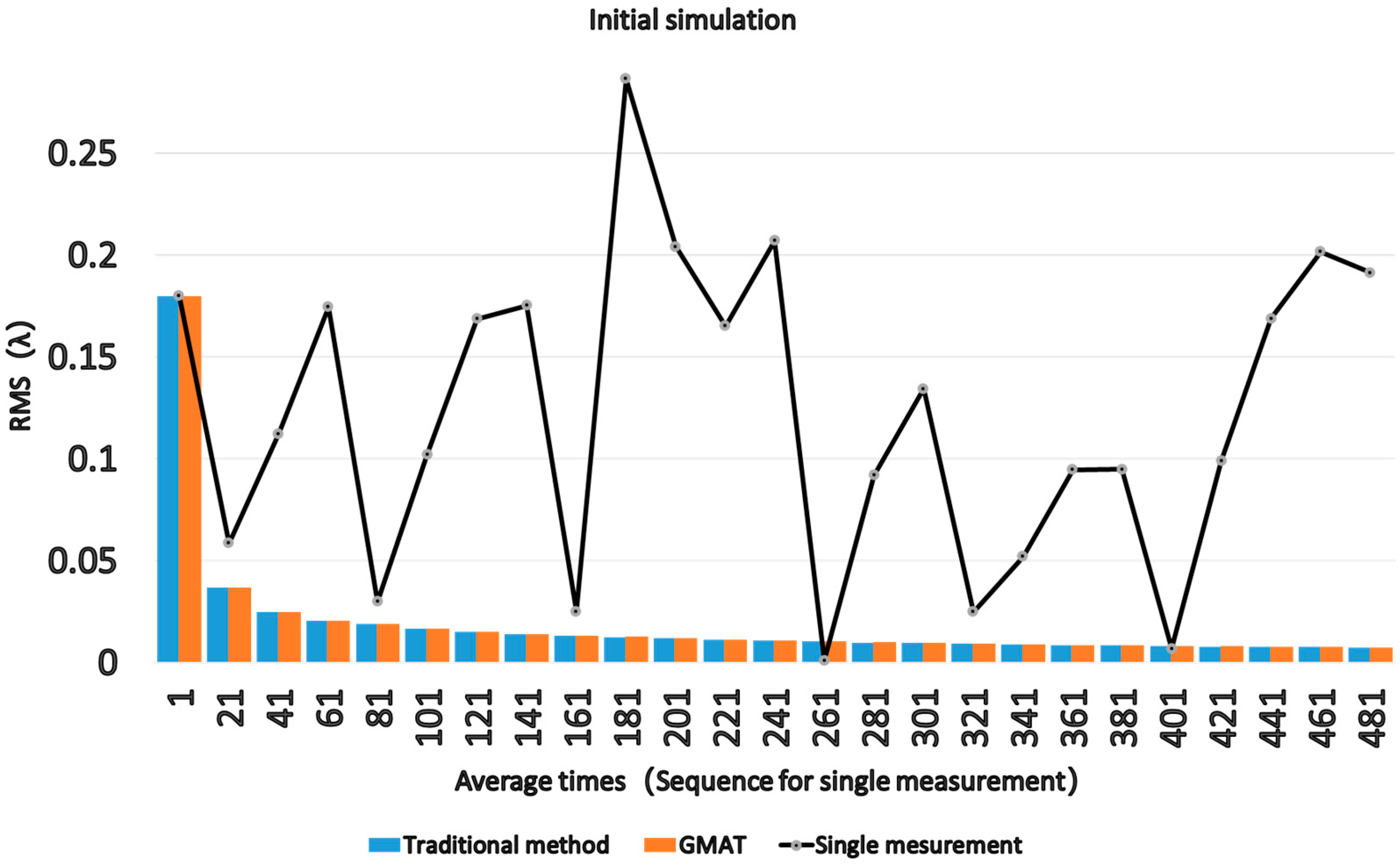
The root-mean-square error (RMSE) and the true values are shown in Figure 5. The blue column shows the results using the traditional method of unwrapping then averaging, and the red color shows the value from the GMAT. The black line shows the results of unwrapping individually. The vertical coordinate is the RMSE, the horizontal coordinate is the average time, and for the black curve, the horizontal coordinate represents the measurement sequence. In this initial configuration, the average SNR of the wrapped phase is 7.635 dB. S N R ¯ is calculated by the following equation:
S N R k = 10 lg i = 1 M j = 1 N ϕ k ¯ i , j 2 i = 1 M j = 1 N ϕ k ¯ i , j G i , j 2 S N R ¯ = k = 1 l S N R k l G k i , j = W R A P P f k x + f y k y + φ
As observed in Figure 5, the red and blue columns have almost the same length and converge gradually with the average times, while the single measurements are significantly random. On the other hand, after 200 averages, the effect of the averaging times is no longer as significant as the first two hundred times, and from the aspect of shortening the measurement process, it is sufficient to collect only 200 sets of data.
Next, the SNR is decreased. Table 1 shows the RMS errors for the GMAT and traditional methods for different SNRs and average times. Table 2 shows the relationship between the average times and the time cost.
It was observed that the conventional method still converges when the noise increases, but it converges to a relatively large value. At this point, it not only fails to remove the noise but also leads to errors. This is due to the fact that as the noise increases, the success rate of unwrapping decreases, and the errors occurring in unwrapping will accumulate and eventually lead to erroneous results. In addition, increasing the number of averages does not yield better results.
The noise will affect which value the circular averaging method eventually converges to and the efficiency of the convergence. Additionally, it can be illustrated from the simulation that the use of the GMAT in low-SNR conditions can help avoid serious effects due to wrongly unwrapping and is more favorable for solving the final phase.

3.2. Analysis of Atmospheric Turbulence

Next, air disturbances are taken into account, and Equation (12) is rewritten to obtain the following equation:
ϕ i ¯ = W R A P P f x i x + f y i y + φ   + n i + A i r i
For short periods, air perturbations are slowly varying and small in magnitude relative to vibrations [22]. It is useful to simulate the air disturbance with Zernike polynomials and to limit the amplitude of other aberrations to ensure that the vibration is the dominant factor affecting the mode. Although the air perturbations are slowly varying, they are random on long time scales. If the interval is long enough, the air disturbances at two time points may be completely different. Assuming that the perturbation between these two points varies linearly, we obtain a model for the air disturbance.
A i r k = A i r j + A i r i A i r j k j i j ,   j k i
where A i r i and A i r j are random aberrations generated with polynomials, and the distance i j is denoted as N . N can reflect the frequency of air changes. We assume that the time interval between each data acquisition is fixed and denote it as T 0 . The time interval between A i r j and A i r i is T, and the frequency of the air disturbance is denoted as f . We obtain Equation (16):
f = 1 T = 1 T 0 N
So, we can tell that N 1 f . The larger N is, the slower the air changes, and vice versa.
When N is 1, A i r is all randomized. The simulation results at this time are shown below. The first row in Figure 6 shows a portion of the wrapped phase, the second row shows the atmospheric perturbations added to it, and the third row shows the GMAT phase.
Figure 7 shows the convergence of the GMAT and conventional methods at different values of N. When N = 1, the GMAT achieves the same results as the traditional method. When N = 2, good average results can still be achieved. The GMAT starts to fail when N = 3 and fails completely when N = 10.
As N increases, the GMAT gradually fails, so in practice, the value of N should be minimized. The solution we give is to elongate the time between two data acquisitions. When the time is long enough, the turbulence between two acquisitions can be considered uncorrelated, and N is exactly 1.
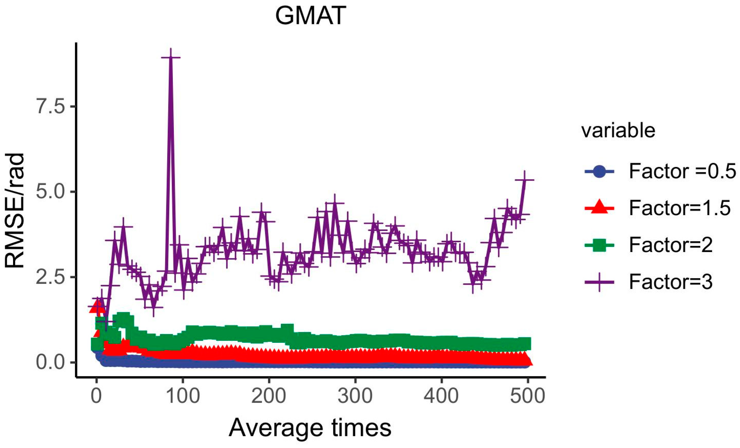
The effect that the magnitude of the air disturbance has on the GMAT is analyzed next. Using the configuration at N = 1 as a baseline, the magnitude of the perturbation is varied by multiplying it by a factor. Figure 8 shows the results of the GMAT when the factor = 0.5, = 1.5, = 2, and = 3, respectively.
With the vibrations removed, the main component of the wrapped phase should be φ, and if the air perturbation is so great that it obscures φ, the circular averaging method will fail. This agrees well with the simulation results; when the coefficient is 0.5, the perturbation is very small compared to φ, and the circular averaging result is very close to that of the conventional method. As the perturbation increases, circular averaging still works but becomes less effective. When the perturbation increases to a certain level, the perturbation becomes the main component, and the circular averaging method is completely ineffective.

3.3. Judgment of Whether We Can Use the GMAT

In order to accurately decide whether or not to use the GMAT, a criterion will be presented in this subsection. In Equation (3), µ is a mean which measures the azimuth, x , and is an average representation of the entire distribution;   κ is a measure of the degree to which the azimuth, x , is concentrated. As κ tends to zero, the distribution is dispersed to be insufficient to satisfy the existence of a mean value for the angle x . As κ tends to infinity, the azimuthal angle is highly concentrated, and it approximates a Gaussian distribution with a mean of μ and a variance of 1 / κ .
f x κ 2 π e κ x μ ^ 2 2
The CDF of the von Mises distribution is displayed in Figure 9 as a straight line when κ = 0, at which point it is completely uniform.
Since the data are dispersed when κ   tends to 0, which does not satisfy the condition for the existence of an angular mean, and perfectly normally distributed when it tends to infinity, it is perfectly acceptable to use this as a criterion to determine whether the GMAT can be applied with wrapped phase data.
Theoretically, there exists a one-dimensional sequence of times at each spatial location, and a maximum likelihood estimation of the von Mises distribution can be performed on this set of data; the parameter estimation operator for κ is given here.
R = 1 n i = 1 n cos x i 2 + i = 1 n sin x i 2 1 2
κ 2 R + R 3 + 5 6 R 5 , w h e n   R < 0.53 0.4 + 1.39 R + 0.43 1 R , w h e n   0.53 < R < 0.85 1 R 3 4 R 2 + 3 R , o t h e r
Since circular averaging will fail when κ is too small, we naturally want κ to be as large as possible. κ is calculated for all positions, and a threshold is set such that those less than this threshold are considered bad points and those greater than this threshold are considered good points. The GMAT is determined to be unapplicable when there are too many bad points. In practice, the application does not need to be solved for all positions; only some of the representative positions need to be extracted.

4. Experiment

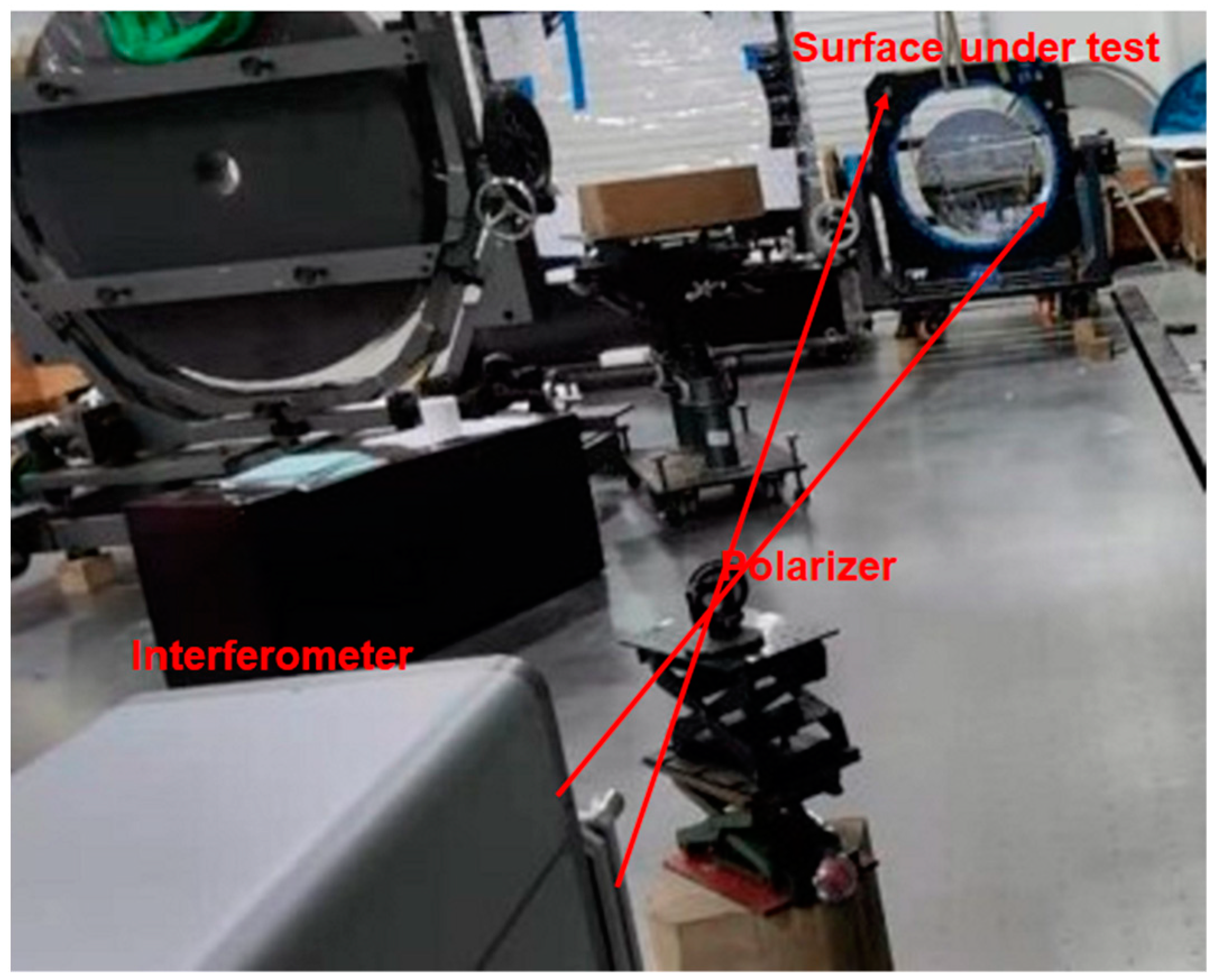
Experiments were carried out on one hundred frames of wrapped phases that were actually measured. Figure 10 shows the physical environment in which the experiment was conducted.
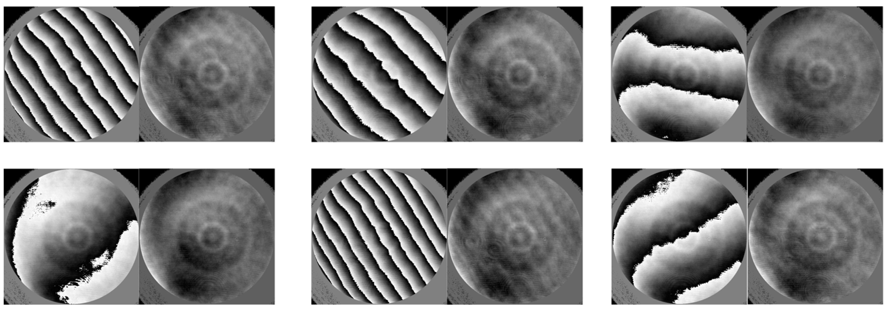
Figure 11 shows some of these and their GMAT-processed phases. The horizontal coordinate in Figure 12 represents the average times, while the vertical coordinate is the residual RMS between the current average times and the results obtained by averaging one hundred times using the traditional method. After GMAT processing, the wrapped phases have identical modes. The average κ value obtained using fifty points is 10.636. On this basis, it can be argued that the GMAT makes all phases up to the prerequisite of performing circular averaging.
Figure 13 shows some of GMAT-processed phases with wrapping included. The RMS of the average phase is shown in Figure 14. The GMAT achieved almost the same results as the traditional method, which demonstrates the validity of it.
Next, we will show the case where there is a wrapping. The blue line deviates slightly from the red line, but we are still able to achieve good results. κ is now 1.59, which is still a good value. In scenarios where the GMAT cannot be applied, κ is usually less than 0.5.

5. Conclusions

The GMAT is able to suppress random noise with only one unwrapping, which greatly reduces the computation time and memory overhead. The more data that participate in the averaging, the more time costs are saved.
Noise and air disturbances can affect the effectiveness of the GMAT. The effect of the SNR on the GMAT was specifically investigated, and the results showed that within a certain SNR range, the GMAT is able to achieve good results. On the other hand, the amplitude and frequency of airflow disturbances can seriously affect the effectiveness of the GMAT.
The judgments presented in this paper can determine which situations are appropriate for the GMAT. For example, in the case of strong airflow effects, the calculated value of κ will be small, and using the GMAT at this point will give rise to the wrong result.

Author Contributions

Conceptualization, Z.T. and F.L.; writing—original draft preparation and experimental work, Z.T.; writing—review and editing, Z.T.; supervision and experimental work, F.L. and Y.W. All authors have read and agreed to the published version of the manuscript.

Funding

This work was supported by the National Key Research and Development Program under Fund No. 2022YFF0712900 and Sichuan Science and Technology Program under Fund No. 22CXRC0017.

Institutional Review Board Statement

Not applicable as the study did not involve human subjects or animals.

Informed Consent Statement

Not applicable as the study did not involve human subjects or animals.

Data Availability Statement

Data underlying the results presented in this paper are not publicly available at this time but may be obtained from the authors upon reasonable request.

Acknowledgments

The authors would like to thank Xiaojun Chen for her helpful discussions.

Conflicts of Interest

The authors declare no conflicts of interest.

References

  1. Liu, F.; Wu, Y.; Chen, Q.; Liu, H.; Yan, F.; Zhang, S.; Wan, Y.; Fan, W. Overview of advanced manufacturing technology of large-aperture aspheric mirror. Opto-Electron. Eng. 2020, 47, 200203. [Google Scholar]
  2. Takeda, M.; Ina, H.; Kobayashi, S. Fourier-transform method of fringe-pattern analysis for computer-based topography and interferometry. J. Opt. Soc. Am. 1982, 72, 156–160. [Google Scholar] [CrossRef]
  3. Smythe, R.; Moore, R. Instantaneous phase measuring interferometry. Opt. Eng. 1984, 23, 361–364. [Google Scholar] [CrossRef]
  4. Kujawinska, M.; Wojciak, J. Spatial-carrier phase-shifting technique of fringe pattern analysis. In Proceedings of the Industrial Applications of Holographic and Speckle Measuring Techniques, Hague, The Netherlands, 11–15 March 1991. [Google Scholar]
  5. Malacara, D. (Ed.) Optical Shop Testing; John Wiley & Sons: Hoboken, NJ, USA, 2007; Volume 59. [Google Scholar]
  6. Ghiglia, D.C.; Pritt, M.D. Two-Dimensional Phase Unwrapping: Theory, Algorithms, and Software, 1st ed.; Wiely-Interscience: Hoboken, NJ, USA, 1998. [Google Scholar]
  7. Aebischer, H.A.; Waldner, S. A simple and effective method for filtering speckle-interferometric phase fringe patterns. Opt. Commun. 1999, 162, 205–210. [Google Scholar] [CrossRef]
  8. Kemao, Q. Two-dimensional windowed Fourier transform for fringe pattern analysis: Principles, applications and implementations. Opt. Lasers Eng. 2007, 45, 304–317. [Google Scholar] [CrossRef]
  9. Agarwal, N.; Chenxing, W.; Qian, K. Windowed Fourier ridges for demodulation of carrier fringe patterns with nonlinearity: A theoretical analysis. Appl. Opt. 2018, 57, 6198–6206. [Google Scholar] [CrossRef] [PubMed]
  10. Jiang, H.; Ma, Y.; Su, Z.; Dai, M.; Yang, F.; He, X. Speckle-interferometric phase fringe patterns de-noising by using fringes’ direction and curvature. Opt. Lasers Eng. 2019, 119, 30–36. [Google Scholar] [CrossRef]
  11. Yan, K.; Yu, Y.; Huang, C.; Sui, L.; Qian, K.; Asundi, A. Fringe pattern denoising based on deep learning. Opt. Commun. 2019, 437, 148–152. [Google Scholar] [CrossRef]
  12. Kim, O.; Rhee, H.; Lee, Y. Dual-path Phase Unwrapping Algorithm Based on Geodesic Curvature for Interferometric Fringe Analysis. J. Korean Phys. Soc. 2020, 76, 202–209. [Google Scholar] [CrossRef]
  13. Baharmast, A.; Kostamovaara, J.T. High-speed wide dynamic range linear mode time-of-flight receiver based on zero-crossing timing detection. Opt. Eng. 2016, 55, 104102. [Google Scholar] [CrossRef]
  14. Liu, B.; Ruan, Y.; Yu, Y. All-Fiber Laser-Self-Mixing Sensor for Acoustic Emission Measurement. J. Light. Technol. 2021, 39, 4062–4068. [Google Scholar] [CrossRef]
  15. Sun, X.; Wang, H.; Liu, B. Measurement of microsurface topography using a self-mixing optical configuration. Opt. Eng. 2018, 57, 051503. [Google Scholar] [CrossRef]
  16. Malacara, Z.; Manuel, S. Interferogram Analysis for Optical Testing; CRC Press: Boca Raton, FL, USA, 2018. [Google Scholar]
  17. Kim, O.; Bong, J.L.; Lee, Y.W.; Yang, H.S. Phase retrieval by pattern classification and circular mean for robust optical testing. Opt. Lasers Eng. 2021, 137, 106304. [Google Scholar] [CrossRef]
  18. Watson, G.S. Distributions on the circle and sphere. J. Appl. Probab. 1982, 19, 265–280. [Google Scholar] [CrossRef]
  19. Fisher, R.A. Dispersion on a sphere. Proc. R. Soc. London. Ser. A Math. Phys. Sci. 1953, 217, 295–305. [Google Scholar] [CrossRef]
  20. Fisher, N.I.; Toby, L.; Embleton, B.J.J. Statistical Analysis of Spherical Data; Cambridge University Press: Cambridge, UK, 1993. [Google Scholar]
  21. Vargas, J.; Quiroga, J.A.; Álvarez-Herrero, A.; Belenguer, T. Phase shifting interferometry based on induced vibrations. Opt. Express 2011, 19, 584–596. [Google Scholar] [CrossRef] [PubMed]
  22. Wang, C.; Liu, J.; Liu, S.; Zheng, Z.; Zhang, H.; Zhang, G. New method for detecting air turbulence. J. Appl. Opt. 2007, 28, 406–411. [Google Scholar] [CrossRef]
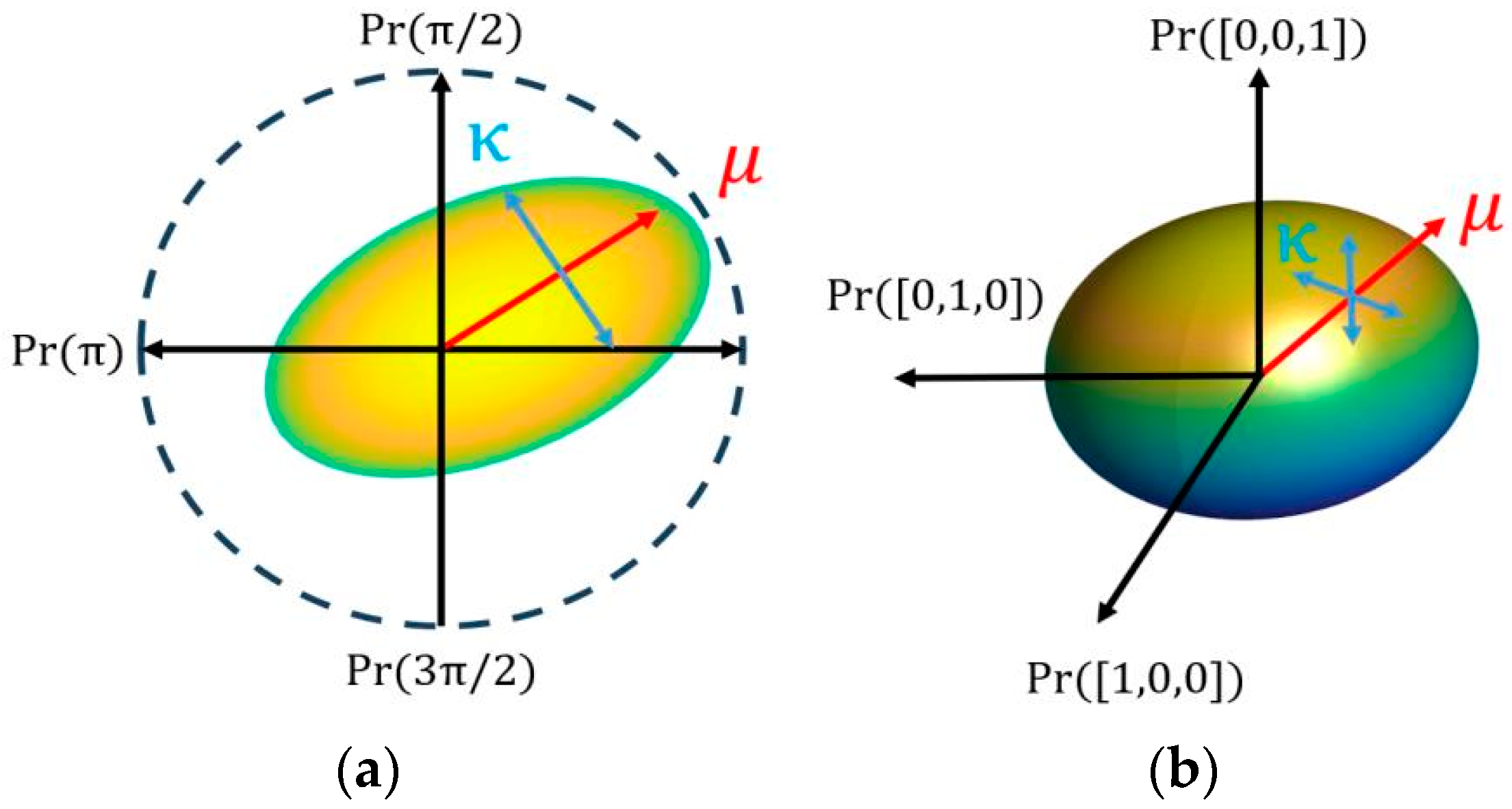
Figure 1. von Mises–Fisher distribution: (a) von Mises distribution; (b) Fisher distribution.
Photonics 11 00561 g001
Figure 2. Wrapped phases of the different modes.
Photonics 11 00561 g002
Figure 3. The process of obtaining the GMAT phase.
Photonics 11 00561 g003
Figure 4. Wrapped phases and GMAT phases.
Photonics 11 00561 g004
Figure 5. Results of initial simulation.
Photonics 11 00561 g005
Figure 6. Simulation results: the first row is the wrapped phase, the second row is the atmospheric perturbation, and the third row is the GMAT phase.
Photonics 11 00561 g006
Figure 7. Results of simulation with different values of N.
Photonics 11 00561 g007
Figure 8. Results of simulation with different factors.
Photonics 11 00561 g008
Figure 9. CDF of the von Mises distribution.
Photonics 11 00561 g009
Figure 10. Experimental environment.
Photonics 11 00561 g010
Figure 11. The case when no wrapping is included in the GMAT phase.
Photonics 11 00561 g011
Figure 12. The result when no wrapping is included in the GMAT phase.
Photonics 11 00561 g012
Figure 13. The case when wrapping is included in the GMAT phase.
Photonics 11 00561 g013
Figure 14. The result when wrapping is included in the GMAT phase.
Photonics 11 00561 g014
Table 1. Simulation results under different noises.
Averaging Times2050100150200
GMAT (SNR)RMS (wave length)
1.579 dB0.0220.0150.0110.0090.007
−1.732 dB0.1850.1290.0950.0830.078
−3.841 dB1.7062.3210.2550.2010.187
Traditional method (SNR)RMS (wave length)
1.579 dB0.0730.0490.0320.0260.023
−1.732 dB2.0361.3550.9190.7970.765
−3.841 dB3.5462.6641.9921.7321.722
Table 2. Computational time.
Averaging Times1251015
Time cost (s)
GMAT2.3842.3872.4022.4742.655
Traditional method2.3724.8411.75522.03434.640
Disclaimer/Publisher’s Note: The statements, opinions and data contained in all publications are solely those of the individual author(s) and contributor(s) and not of MDPI and/or the editor(s). MDPI and/or the editor(s) disclaim responsibility for any injury to people or property resulting from any ideas, methods, instructions or products referred to in the content.