Compressed Sensing Image Reconstruction with Fast Convolution Filtering

Abstract

Image reconstruction is a crucial aspect of computational imaging. The compressed sensing reconstruction (CS) method has been developed to obtain high-quality images. However, the CS method is commonly time-consuming in image reconstruction. To overcome this drawback, we propose a compressed sensing reconstruction method with fast convolution filtering (F-CS method), which significantly increases reconstruction speed by reducing the number of convolution operations without image fill. The experimental results show that by using the F-CS method, the reconstruction speed can be increased by a factor of 7 compared to the conventional CS method. Moreover, the F-CS method proposed in this paper is compared with the back-propagation reconstruction (BP) method and super-resolution reconstruction (SR) method, and it is validated that the proposed method has a lower computational resource cost for high-quality image reconstruction and exhibits a much more balanced capability.

1. Introduction

Computational imaging has been rapidly developed from coherent diffractive imaging in recent years due to its high flexibility and reduced limitation of optical components [1,2,3,4], with wide application prospects for biomedical imaging, virtual reality, and remote sensing, etc. As an indispensable aspect, image reconstruction is of great importance for computational imaging and other image-related applications [5,6,7,8,9], which can transform collected signals into visual images with increased resolution and noise reduction. Furthermore, image reconstruction should be able to meet a variety of imaging requirements such as fast imaging, high-resolution imaging, and low-dose imaging.

As a new type of signal sampling and reconstruction theory, compressed sensing (CS) was proposed in 2006 [10]. The main content of the CS theory is the reconstruction of large dimensional signals from a small number of samples by means of the signal sparsity, which overcomes the limitation imposed by the Nyquist–Shannon theorem. CS employs sparsity of the original signal to realize reconstruction with only a few non-zero coefficients on a suitable basis [11]. On the premise of ensuring reconstruction accuracy, the CS method can effectively reduce the sampling complexity and data storage amount [12]. Compared with the conventional sampling method, the CS method greatly improves the sampling efficiency. It is especially suitable for signal processing with high dimensions, high complexity, and a large data amount.

Due to the advantages of the CS theory, in recent years, scholars have conducted extensive research on it and proposed various CS-based reconstruction methods. Needell [13] developed a total variation minimization algorithm, which can reconstruct images by minimizing the total variation in all image blocks. Iterative threshold algorithms [14] were proposed to gradually approximate and reconstruct the signal by iteratively calculating the main coefficients in the original signal; while evaluating the difference between the reconstructed signal and the original signal in each iteration, the reconstruction accuracy can be increased by continuously reducing the gap with sparse original signals. The orthogonal matching pursuit (OMP) algorithm was born by analyzing the part of the observation matrix that has the highest correlation with the original sparse signal. This further improves the accuracy of signal reconstruction [15]. Kulkarni [16] developed the classical algorithm ReconNet based on a convolutional neural network, and it can directly reconstruct the original images into compressed sensing measurements enhancing the image reconstruction efficiency. Next, Yao [17] proposed the deep residual network (DR²-Net) on the basis of ReconNet, which applied the residual network to the compressed sensing image reconstruction. Du [18] launched the full convolutional measurement network (FCMN), and Sun [19] proposed the DPA-Net method combined with the attention mechanism to optimize image reconstruction. All these efforts have driven the improvement of the CS reconstruction method.

At present, the compressed sensing reconstruction methods are generally able to reconstruct images of high quality and have flexible usage conditions. However, these methods also have an obvious problem of low reconstruction efficiency. The reconstruction process involves numerous steps and requires a significant amount of time and computational resources.

To address the above issue, this study proposes a compressed sensing reconstruction method with fast convolution filtering (F-CS method) to greatly increase the reconstruction speed. Section 2 introduces the principle and optimization of the F-CS method. Experiments are conducted for validation by comparing the F-CS method with various conventional reconstruction methods, as described in Section 3. The experimental results are investigated and demonstrate that our method significantly enhances reconstruction speed.

2. Principle and Optimization

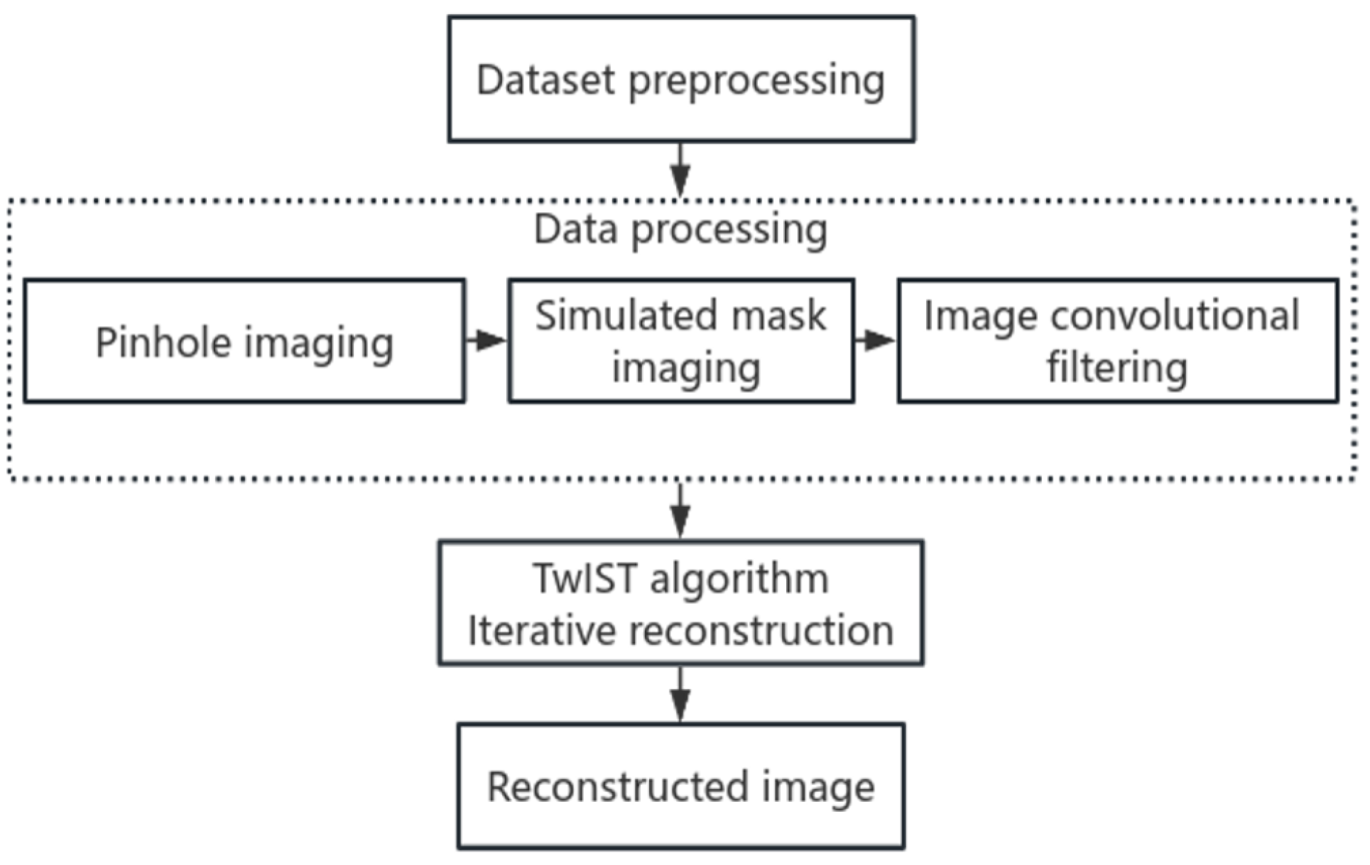
2.1. Principle of Compressed Sensing Reconstruction

The compressed sensing reconstruction algorithm is developed based on data collection according to the Nyquist–Shannon sampling theorem and fast Fourier transform. Utilizing the nature of discreteness, a pulse function $\delta \left(t\right)$ with a sampling period of $T_s$ and a length of n can be used to represent the periodic sampling function $P\left(t\right)$ by [20]

$$P\left(t\right)=\sum _{n=-\infty }^{+\infty }\delta \left(t-n{T}_s\right).$$

(1)

The sampling of an original signal $x\left(t\right)$ is conducted by using $P\left(t\right)$, and thereby the discrete signal $x_s\left(t\right)$ can be expressed as

$$x_s\left(t\right)=\sum _{n=-\infty }^{+\infty }x\left(t-n{T}_s\right).$$

(2)

With ${\omega }_s=2\pi /T_s$, if the Fourier transform of $x\left(t\right)$ is $F\left(\omega \right)$, the Fourier transform $F_s\left(\omega \right)$ of $x_s\left(t\right)$ can be described by

$$F_s\left(\omega \right)=\frac{1}{T}\sum _{n=-\infty }^{+\infty }F\left(\omega -n{\omega }_s\right).$$

(3)

A Fourier transform domain is used for sparsifying the signal, which is necessary for the compressed sensing reconstruction. In this case, a certain orthogonal transformation basis needs to be introduced to make the original signal sparse. For the original signal $x\in R^N$, $\psi$ is assumed as a set of orthogonal bases $\psi =[{\psi }_1,{\psi }_2\dots {\psi }_N]$ in $R^N$. Then, x can be described as

$$x=\sum _{i=1}^N{\psi }_i{\alpha }_i=\psi \alpha .$$

(4)

$\alpha =[{\alpha }_1,{\alpha }_2\dots {\alpha }_N]$ is the vector of the transformation coefficient and is the sparse representation of the signal x on the orthogonal transformation basis. We introduce the measurement matrix $\Phi \in R^{M\times N}$ with $M\ll N$. The measured values of compressed sensing are expressed as $y\in R^M$. Thus,

$$y=\Phi x.$$

(5)

Considering the expansion of x, it can be written as

$$y=\Phi \psi \alpha .$$

(6)

The compressed sensing reconstruction requires that the measurement matrix meets the restricted isometry property (RIP). That is, any M column vector in the measurement matrix can form a non-singular matrix. Therefore, the RIP can ensure the measurement matrix does not map different sparse signals into the same transformation domain. It means the original signal space corresponds to the unique sparse space, and different observations can be achieved for a high-quality reconstruction of the image. If $k=1,2,3,\dots ,n$ and the isometric coefficient ${\delta }_k$ of the measurement matrix is minimum, the RIP can be expressed by

$$\left(1-{\delta }_k\right){∥x∥}_2^2\ll {∥\Phi x∥}_2^2\ll \left(1+{\delta }_k\right){∥x∥}_2^2.$$

(7)

When the process runs to this step, the reconstruction image can be achieved by inputting the measured values y of compressed sensing into the reconstruction algorithm. The original signal $x\in R^N$ is reversibly solved via the measured value $y\in R^M$ and the orthogonal transformation basis $\psi$. However, the values obtained through reverse solving may not be unique, and regularization terms for sparsity constraints and, thus, for reducing the number of solutions need to be introduced. The regularization can be realized by L1 norm regularization [21]. When meeting the RIP condition, sparse signals $\alpha$ can be obtained by finding the minimum L1 norm. Inverse transformation is then performed to achieve the reconstruction signal $\widehat{x}$. The process yields

$$\underset{x}{\min }{∥\alpha ∥}_{1}s.t.y=\Phi \widehat{x}=\Phi \psi \alpha ,$$

(8)

where ${∥\alpha ∥}_1$ indicates its L1 norm.

2.2. Optimization of Compressed Sensing Reconstruction

A compressed sensing reconstruction method was developed with a simulation algorithm using a Fourier zone aperture (FZA) for single lens imaging. In the process of image reconstruction, this method can not only simulate the imaging process of the original image on the detector but also show the distance between the image and the lens. The reconstruction process is shown in Figure 1.

The beginning of compressed sensing reconstruction is preprocessing of data, which reads the images in the dataset and inputs the image data into the data processing module group.

The first module of compressed sensing data processing is the pinhole imaging module, which enables the distance effect of the original image in front of the lens to be simulated. Assuming the object is placed in front of the FZA at a distance of $z_1$ and the distance between the FZA and the image sensor is $z_2$, if the height of the object is $h_o$ and the imaging height is $h_I$, the magnification $M_I$ of the pinhole imaging is

$$M_I=\frac{h_I}{H_o}=\frac{z_2}{z_1}.$$

(9)

As the discrete signal $x_s$, the input original image $I(\dot{x},\dot{y})$ is then interpolated to $I(\tilde{x},\tilde{y})$.

The second module of data processing is a simulation mask imaging module, which is mainly to imitate the image projected by the FZA mask. It can stack with the original image, so that each pixel and its neighborhood has a unique feature mark. If the innermost region radius of the FZA is $r_1$ and the radial distance from the aperture center is r, a mask factor matrix can be given by

$$K(\tilde{i},\tilde{j})=\sum \sum \frac{1}{2}\left[1+cos\frac{\pi r^2}{r_1^2}\right].$$

(10)

Next, the mask factor matrix $K(\tilde{i},\tilde{j})$ is used as the convolution kernel to convolve with the image $I(\tilde{x},\tilde{y})$, where $(\tilde{i},\tilde{j})$ and $(\tilde{x},\tilde{y})$ represent the spatial coordinates of the convolution kernel and the image, respectively. The gray value variation in each pixel in the image can thus be calculated. However, the conventional convolution is time-consuming and occupies considerable computational resources. Therefore, here, a two-dimensional fast convolution filtering method is introduced for the first time into compressed sensing reconstruction to replace the conventional convolution and, thus, to optimize reconstruction speed.

When the size of the input image $I(\tilde{x},\tilde{y})$ is $H_I\times W_I$ and the size of the convolution kernel $K(\tilde{i},\tilde{j})$ is $H_K\times W_K$, the principle of the fast convolution filtering can be written as

$$O(\tilde{x},\tilde{y})=\sum \sum K(\tilde{i},\tilde{j})\times I(\tilde{x}+\tilde{i}-H_K/2,\tilde{y}+\tilde{j}-W_K/2),$$

(11)

in which $\sum \sum$ represents the multiplication and summation operation of all elements of the convolution kernel and the corresponding pixels in the input image. The coordinates $(\tilde{x}+\tilde{i}-H_K/2,\tilde{y}+\tilde{j}-W_K/2)$ are the corresponding positions of the convolution kernel on the input image. That is to say, this convolution operation multiplies each element of the convolution kernel with the corresponding pixel. Therefore, the number of computations is $H_I\times W_I\times H_K\times W_K$. Then, all the results are summed to obtain the pixel values of the corresponding positions in the output image.

For conventional convolution operations, the input image boundary should be filled to ensure the sizes of the input and output images remain consistent. Besides $H_K\times W_K$ multiplication operations at each pixel, each multiplication operation must be multiplied by $H_K\times W_K$ weights of the convolution kernel, and the results are accumulated. Thereby, the computation count of traditional convolution operations is $H_I\times W_I\times H_K\times W_K\times (H_K+W_K)$. Obviously, compared to the conventional convolution, the optimized fast convolution has much higher computation speed, which will be validated by the following experimental results.

Finally, a two-step iterative shrinkage/thresholding (TwIST) algorithm [22] is used for the image signal reconstruction. The TwIST algorithm can improve the convergence speed and provide L1 norm regularization. The convolution filtered image data are used as input to the TwIST algorithm, and the TwIST algorithm iteratively approximates the original image by alternating two steps during the iterative process. The first step is to update the coefficient vector by iteratively using the proximal operator. The second step is to sparsify the coefficient vectors by applying a threshold function. This reversible sparsification process guarantees the obtained solutions are sparse and, thus, ensures the quality of the image reconstruction. Consequently, a compressed sensing reconstruction with fast convolution filtering (F-CS) is developed.

3. Experimental Results and Discussion

In the experiments, the performance of F-CS is compared with that of the compressed sensing reconstruction (CS) without fast convolution, back-propagation reconstruction (BP) [23] and super-resolution reconstruction (SR) [24]. As the reference method, BP is an effective technique used in the field of image reconstruction, particularly in the context of computed tomography imaging. It involves the iterative process of refining an initial image reconstruction by propagating the error backward through the imaging system. SR is used in image reconstruction to enhance the resolution of an image beyond its original resolution. It aims to generate a high-resolution image from one or more low-resolution images or from a single low-resolution image. All the image reconstruction algorithms involved in this paper are implemented by using Python with a computer (Intel(R) Core(TM) i7-9750H CPU @ 2.60 GHz, RAM 8.00 GB, GPU NVIDIA GeForce GTX 1650).

The LabelMe-12-50k dataset (url: www.kaggle.com/datasets/dschettler8845/labelme-12-50k, accessed on 20 April 2023) is employed to test the applicability of the reconstruction methods for various images ensuring the training accuracy of relevant models. This dataset is a subset of the LabelMe dataset developed by Massachusetts Institute of Technology (MIT). It contains a total of 50,000 images, including 40,000 for training and 10,000 images for testing. $50\%$ of the image subjects in the training and test sets are in center positions, while the remaining $50\%$ are in randomly selected image regions. In addition, each image is annotated with the semantic level and instance level including up to 12 categories of humans, animals, vehicles, architecture, and landscapes, as well as accurate information such as bounding boxes and masks. Note that the images are selected for direct visualization comparisons in this paper due to their sharp light and dark areas as well as distinctive subjects.

3.1. Design of Evaluation Criteria

In order to objectively evaluate the performance of different methods, the resolution, mean square error ($MSE$), peak signal-to-noise ratio ($PSNR$), and structural similarity ($SSIM$) are used as evaluation indicators for comparative analysis. $MSE$ is commonly used in various fields such as statistics, machine learning, signal processing, and image processing to assess the accuracy of models or algorithms. A lower MSE indicates better predictive performance, as it signifies smaller deviations between predicted and actual values. SSIM is utilized to evaluate the image similarity with brightness, contrast and structure. The similarity of two images is higher with a higher $SSIM$. PSNR is based on the maximum possible value $MAX$ and mean square error of image pixels, which reads

$$PSNR=20\times lg\left(\frac{MAX}{\sqrt{MSE}}\right).$$

(12)

The image distortion is smaller with a higher $PSNR$. The usage rate of CPU, RAM, and GPU will be evaluated for the analysis of the occupation of computational resources.

The mean option score (MOS) [25] is used as the subjective evaluation index to quantify the reconstruction effect of diverse methods. The specific evaluation operation is that 20 examiners should use 1 to 5 points to score the image quality with the premise of unknown image version. The image quality is better with a higher score, and finally the mean score is taken as the subjective evaluation index.

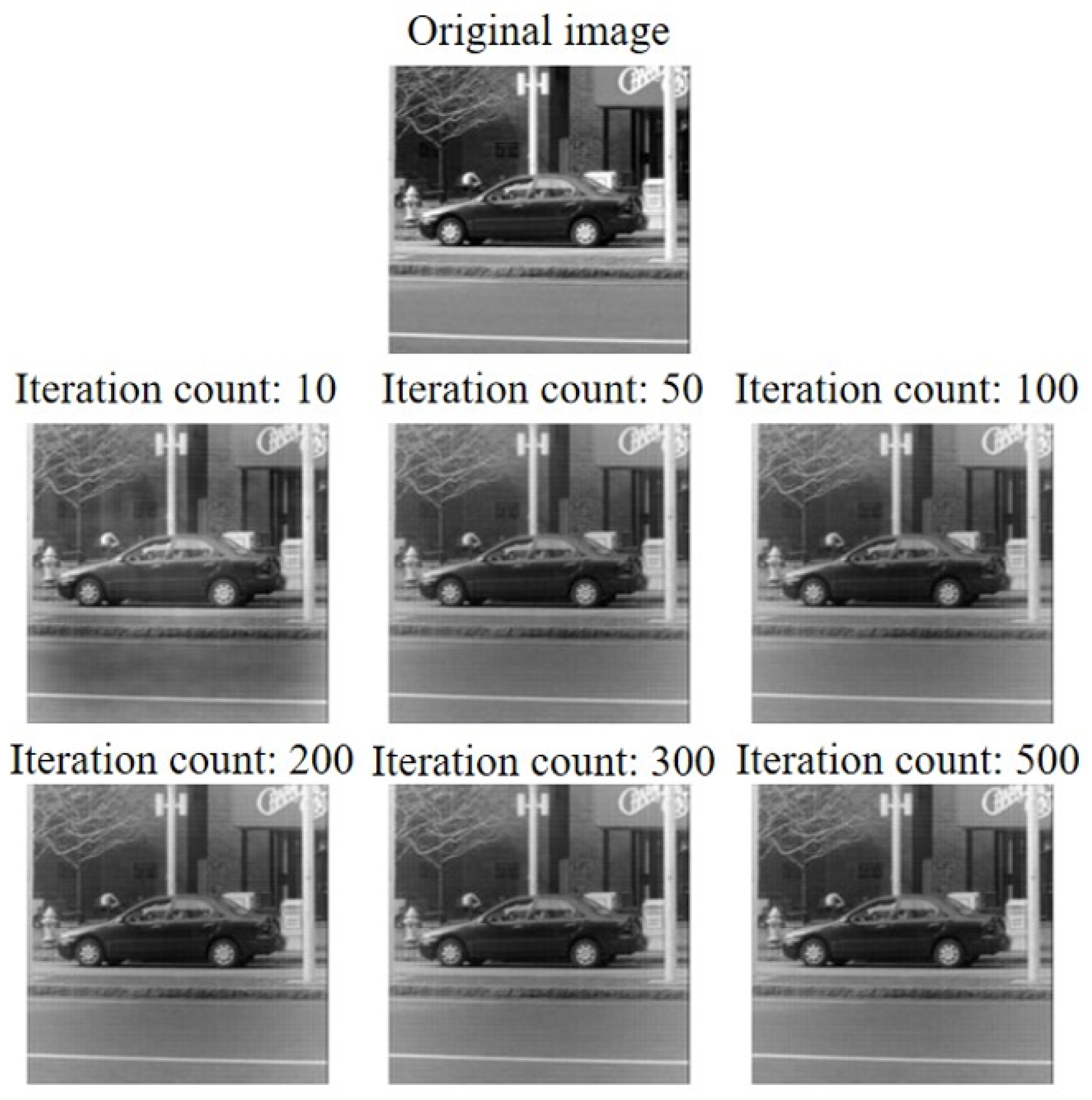
3.2. Performance of Compressed Sensing Reconstruction with Fast Convolution Filtering

In compressed sensing image reconstruction, the quality of image reconstruction is largely determined by iterations. Too few iterations will cause the algorithm not to converge to optimum, while too many iterations is time-consuming. The experimental results of image reconstruction for different numbers of iterations are shown in Figure 2.

It depicts that the image reconstructed with 10 iterations is far from the original image in terms of clarity and brightness, which indicates too few iterations. With 200 or 300 iterations, the reconstruction images almost show no difference from the image at 500 iterations, and they are closer to the original image.

In order to intuitively compare reconstruction quality, the $MSE$, $PSNR$, and $SSIM$ of the reconstruction images and original images with varying numbers of iterations were evaluated. The results are listed in

Table 1. Evaluation parameters of image reconstruction for different numbers of iterations.

Iterations	10	50	100	200	300	500
$MSE$	932.75	675.22	659.60	613.53	555.17	456.28
$PSNR$ (dB)	18.43	19.84	19.94	20.25	20.69	21.54
$SSIM$	0.79	0.82	0.82	0.82	0.83	0.84

.

As can be seen from the results, $MSE$ gradually decreases as the iterations increase, but the decrease rate gradually slows down, while $PSNR$ and $SSIM$ gradually improve, and the quality of the reconstruction images constantly becomes better.

In order to further verify the capability of the F-CS method, three datasets containing different sample sizes were reconstructed by using the F-CS method and the CS method. To highlight the changes in reconstruction speed, the image data were preprocessed. We randomly selected several images from the image database and divided them into three datasets with different sample sizes. The images were preloaded from the same dataset into a file (.npz) for a simple direct reading, and the image reconstruction process was then carried out. The experimental results are shown in

Table 2. Evaluation parameters of image reconstruction with the F-CS and CS methods.

CS	Sample Size	Resolution	$\mathit{MSE}$	$\mathit{PSNR}$ (dB)	$\mathit{SSIM}$	Time (s)
	1	$256\times 256$	3517.651	12.668	0.562	35.407
	20	$256\times 256$	3545.595	12.921	0.523	689.741
	50	$256\times 256$	3221.781	13.445	0.530	1797.955
F-CS	Sample Size	Resolution	$\mathit{MSE}$	$\mathit{PSNR}$ (dB)	$\mathit{SSIM}$	Time (s)
	1	$256\times 256$	3541.930	12.638	0.573	4.831
	20	$256\times 256$	3524.768	12.952	0.533	89.822
	50	$256\times 256$	3186.801	13.495	0.541	229.565

.

The evaluation parameters of the reconstruction results indicate that due to the optimization of the fast convolution filtering in F-CS method, the time of reconstruction has been greatly reduced. The reconstruction speed is increased by about factor 7 compared to the CS method. Meanwhile, the other image quality parameters are also improved. These validate that the proposed F-CS method is effective to enhance the image reconstruction efficiency and quality.

3.3. Comparison of Objective Indicators between Different Reconstruction Methods

The objective comparison analysis of the F-CS, BP, SR methods is conducted using the uniform criteria. Three standard datasets are divided by the number of images, which have small, medium and large quantities. The performances of the three methods are tested with the standard datasets. The reconstruction results of the same original image by utilizing the three methods are illustrated in Figure 3.

It can be seen that compared with the BP result, the F-CS result shows much higher image reconstruction quality. The SR method also offers an effective reconstruction, but it is difficult to conduct a visual comparison with the F-CS method. Therefore, nine objective evaluation parameters of the reconstruction results were computed and are listed in

Table 3. Evaluation parameters of image reconstruction with the F-CS, BP, and SR methods.

F-CS	Sample Size	Resolution	$\mathit{MSE}$	$\mathit{PSNR}$ (dB)	$\mathit{SSIM}$	Time (s)	CPU Usage Rate	RAM Usage Rate	GPU Usage Rate
	1	$128\times 128$	2845.28	13.56	0.74	5.15
	20	$128\times 128$	1868.85	18.57	0.83	101.16	15.1%	12.9%	0%
	50	$128\times 128$	1381.65	18.11	0.83	254.15
BP	Sample Size	Resolution	$\mathit{MSE}$	$\mathit{PSNR}$ (dB)	$\mathit{SSIM}$	Time (s)
	1	$128\times 128$	6114.53	10.27	0.37	0.06
	20	$128\times 128$	4889.76	12.27	0.48	1.53	7.0%	11.0%	0%
	50	$128\times 128$	4480.22	12.29	0.51	3.48
SR	Sample Size	Resolution	$\mathit{MSE}$	$\mathit{PSNR}$ (dB)	$\mathit{SSIM}$	Time (s)
	1	$128\times 128$	166.61	25.91	0.78	2.82
	20	$128\times 128$	272.85	25.86	0.89	43.80	17.4%	67.2%	15%
	50	$128\times 128$	509.01	22.89	0.75	122.36

for comparison.

The evaluation parameters reveal that the BP method offers a relatively low image reconstruction quality in the test, which can be due to the twin image effect. On the other hand, it is very obvious that the reconstruction speed of the BP method is very high. Therefore, the BP method is suitable for the situations where a large number of images need to be reconstructed quickly and the requirement of reconstruction quality is low.

Regarding the SR method, the $MSE$ of pixels is small and has a high $PSNR$, and its reconstruction process has a significant inhibitory effect on the noise. However, due to numerous parameters in model training, the SR method is resource-consuming and has high RAM and GPU usage in the image reconstruction.

The F-CS method exhibits high structural similarity when reconstructing a same dataset. Although it is relatively time-consuming, the reconstruction speed of the F-CS method has already been significantly increased compared with the conventional CS method as mentioned in Section 3.2. In comparison to the SR method, the F-CS method does not require the construction of high complexity models, which saves computational resources. This makes it much easier achieve image reconstruction meeting high-resolution requirements. Meanwhile, as the limitations, the $MSE$ and $PSNR$ of the F-CS-based image reconstruction still need to be improved compared to those when using the SR method.

Consequently, the F-CS method proposed in this paper greatly improves the speed of image reconstruction compared to the CS methods that do not use the fast convolution [13,14,15]. Compared with the BP method [23], using the F-CS method can significantly improve the reconstruction quality. Compared to the AI-driven methods [16,17,18,19,24], the F-CS method enables large amounts of RAM and GPU resources to be saved and more conveniently obtains high-quality reconstruction images without training model. Thus, the F-CS method exhibits much balanced performances in terms of reconstruction speed and quality, as well as consumption of computational resources.

3.4. Comparison of Subjective Indicators between Different Reconstruction Methods

The mean option score (MOS) is used as a subjective evaluation index for comparing the image reconstruction quality. Twenty images to be evaluated are in the form of Figure 3. The positions of the reconstruction images on each comparison map are disrupted, and the reconstruction category logo is erased while retaining only the logo of the original images. Twenty judges were asked to anonymously score the quality of each reconstruction image using five score grades of 1–5. The 20 judges are all young people aged 20–23. They completed the scoring separately in sequence. There was no communication during the scoring process, and all images were displayed on the same computer. All scoring results were summarized to obtain the average score for each image reconstructed by using the three methods, as shown in

Table 4. Mean option score of reconstruction image quality.

Reconstruction Image	1	2	3	4	5	6	7	8	9	10	11	12	13	14	15	16	17	18	19	20
F-CS	3.3	3.7	3.7	3.55	3.55	3.45	3.65	4.75	3.5	3.65	3.3	3.35	3.4	3.55	3.55	3.35	3.4	3.45	3.45	4.35
BP	1.6	3.55	3.7	1.5	3.55	3.6	3.3	1.7	1.4	1.35	1.5	3.55	1.65	1.4	3.6	1.5	3.55	1.45	1.45	3.45
SR	4.6	4.4	3.45	3.45	3.45	3.4	4.65	3.45	3.55	3.45	3.5	3.55	3.3	3.75	4.5	3.55	3.35	3.55	3.4	3.35

.

Through data statistics, the mean option scores of the reconstruction images by using the F-CS, BP, and SR methods are 3.60, 2.42, and 3.68, respectively. It can be seen that from the perspective of human eye observation, the reconstruction quality of the BP method is still low, and the reconstruction quality of the SR method is slightly 0.08 points higher than that of the F-CS method, which is very close to the analysis results achieved under objective standards.

From the comparative analysis of the subjective and objective evaluations, it is revealed that the combination of subjective and objective evaluations can more comprehensively reflect the quality of image reconstruction.

4. Conclusions

In this paper, a compressed sensing reconstruction method with fast convolution filtering (F-CS method) is proposed. The fast convolution filtering can greatly reduce the number of convolution operations and, thus, increase the reconstruction speed. The experimental results indicate, compared to the CS method that does not use the fast convolution, that the image reconstruction speed of the F-CS method is increased by a factor of 7. Furthermore, the objective and subjective evaluations shows that the F-CS method has a lower computational resource cost for high-quality image reconstruction compared with the BP and SR methods.

In further work, the F-CS method will be applied to computational imaging such as laser speckle imaging and biomedical imaging. The fast convolution filtering can also be used in other signal reconstruction methods that are limited by the convolution speed.

References

1. Miao, J.; Charalambous, P.; Kirz, J.; Sayre, D. Extending the methodology of X-ray crystallography to allow imaging of micrometre-sized non-crystalline specimens. Nature 1999, 400, 342–344. [Google Scholar] [CrossRef]
2. Marchesini, S.; He, H.; Chapman, H.N.; Hau-Riege, S.P.; Noy, A.; Howells, M.R.; Weierstall, U.; Spence, J.C. X-ray image reconstruction from a diffraction pattern alone. Phys. Rev. B 2003, 68, 140101. [Google Scholar] [CrossRef]
3. Rodenburg, J.M. Ptychography and related diffractive imaging methods. Adv. Imaging Electron Phys. 2008, 150, 87–184. [Google Scholar]
4. Zheng, G.; Horstmeyer, R.; Yang, C. Wide-field, high-resolution Fourier ptychographic microscopy. Nat. Photonics 2013, 7, 739–745. [Google Scholar] [CrossRef] [PubMed]
5. Gao, Z.; Radner, H.; Büttner, L.; Ye, H.; Li, X.; Czarske, J. Distortion correction for particle image velocimetry using multiple-input deep convolutional neural network and Hartmann-Shack sensing. Opt. Express 2021, 29, 18669–18687. [Google Scholar] [CrossRef] [PubMed]
6. Zhang, H.; Kuschmierz, R.; Czarske, J.; Fischer, A. Camera-based speckle noise reduction for 3-D absolute shape measurements. Opt. Express 2016, 24, 12130–12141. [Google Scholar] [CrossRef] [PubMed]
7. Zhang, H.; Kuschmierz, R.; Czarske, J. Miniaturized interferometric 3-D shape sensor using coherent fiber bundles. Opt. Lasers Eng. 2018, 107, 364–369. [Google Scholar] [CrossRef]
8. Kuschmierz, R.; Scharf, E.; Ortegón-González, D.F.; Glosemeyer, T.; Czarske, J.W. Ultra-thin 3D lensless fiber endoscopy using diffractive optical elements and deep neural networks. Light Adv. Manuf. 2021, 2, 415–424. [Google Scholar] [CrossRef]
9. Zhang, H. Laser interference 3-D sensor with line-shaped beam based multipoint measurements using cylindrical lens. Opt. Lasers Eng. 2022, 159, 107218. [Google Scholar] [CrossRef]
10. Candès, E.J.; Romberg, J.; Tao, T. Robust uncertainty principles: Exact signal reconstruction from highly incomplete frequency information. IEEE Trans. Inf. Theory 2006, 52, 489–509. [Google Scholar] [CrossRef]
11. Pilastri, A.L.; Tavares, J.M.R. Reconstruction algorithms in compressive sensing: An overview. In Proceedings of the 11th Edition of the Doctoral Symposium in Informatics Engineering (DSIE-16), Porto, Portugal, 3 February 2016. [Google Scholar]
12. Donoho, D.L. Compressed sensing. IEEE Trans. Inf. Theory 2006, 52, 1289–1306. [Google Scholar] [CrossRef]
13. Needell, D.; Ward, R. Stable image reconstruction using total variation minimization. SIAM J. Imaging Sci. 2013, 6, 1035–1058. [Google Scholar] [CrossRef]
14. Zhu, T. New over-relaxed monotone fast iterative shrinkage-thresholding algorithm for linear inverse problems. IET Image Process. 2019, 13, 2888–2896. [Google Scholar] [CrossRef]
15. Pati, Y.C.; Rezaiifar, R.; Krishnaprasad, P.S. Orthogonal matching pursuit: Recursive function approximation with applications to wavelet decomposition. In Proceedings of the 27th Asilomar Conference on Signals, Systems and Computers, Pacific Grove, CA, USA, 1–3 November 1993; pp. 40–44. [Google Scholar]
16. Kulkarni, K.; Lohit, S.; Turaga, P.; Kerviche, R.; Ashok, A. Reconnet: Non-iterative reconstruction of images from compressively sensed measurements. In Proceedings of the IEEE Conference on Computer Vision and Pattern Recognition, Las Vegas, NV, USA, 27–30 June 2016; pp. 449–458. [Google Scholar]
17. Yao, H.; Dai, F.; Zhang, S.; Zhang, Y.; Tian, Q.; Xu, C. Dr2-net: Deep residual reconstruction network for image compressive sensing. Neurocomputing 2019, 359, 483–493. [Google Scholar] [CrossRef]
18. Du, J.; Xie, X.; Wang, C.; Shi, G.; Xu, X.; Wang, Y. Fully convolutional measurement network for compressive sensing image reconstruction. Neurocomputing 2019, 328, 105–112. [Google Scholar] [CrossRef]
19. Sun, Y.; Chen, J.; Liu, Q.; Liu, B.; Guo, G. Dual-path attention network for compressed sensing image reconstruction. IEEE Trans. Image Process. 2020, 29, 9482–9495. [Google Scholar] [CrossRef]
20. Lesnikov, V.; Naumovich, T.; Chastikov, A. Analysis of Periodically Non-Uniform Sampled Signals. In Proceedings of the 2022 24th International Conference on Digital Signal Processing and its Applications (DSPA), Moscow, Russian, 30 March–1 April 2022; pp. 1–4. [Google Scholar]
21. Li, C. An Efficient Algorithm for Total Variation Regularization with Applications to the Single Pixel Camera and Compressive Sensing. Master’s Thesis, Rice University, Houston, TX, USA, 2010. [Google Scholar]
22. Bioucas-Dias, J.M.; Figueiredo, M.A. A new TwIST: Two-step iterative shrinkage/thresholding algorithms for image restoration. IEEE Trans. Image Process. 2007, 16, 2992–3004. [Google Scholar] [CrossRef]
23. Devaney, A.J. A filtered backpropagation algorithm for diffraction tomography. Ultrason. Imaging 1982, 4, 336–350. [Google Scholar] [CrossRef] [PubMed]
24. Park, S.C.; Park, M.K.; Kang, M.G. Super-resolution image reconstruction: A technical overview. IEEE Signal Process. Mag. 2003, 20, 21–36. [Google Scholar] [CrossRef]
25. Kumar, B.; Singh, S.P.; Mohan, A.; Anand, A. Performance of quality metrics for compressed medical images through mean opinion score prediction. J. Med. Imaging Health Inform. 2012, 2, 188–194. [Google Scholar] [CrossRef]
Figure 1. Scheme of a compressed sensing image reconstruction.
Photonics 11 00323 g001
Figure 2. Reconstruction images with various iterations.
Photonics 11 00323 g002
Figure 3. Reconstruction images with the F-CS, BP, and SR methods.
Photonics 11 00323 g003