1. Introduction
In laser communication, the phenomenon of turbulence in the atmosphere has serious interference with the laser beam, which in turn affects the signal-to-noise ratio and bit error rate in laser communication [
1]. This is due to the fact that atmospheric turbulence causes variations in the intensity and phase of the laser light, and these variations seriously affect the imaging quality of the beacon spot and the communication spot, leading to a reduction in pointing accuracy and communication quality [
2].
In order to reduce the effect of atmospheric turbulence on the beam in laser communication, an adaptive optics tracking system is generally used to realize high-precision capture and tracking of the beacon light [
3]. The adaptive optics tracking system allows the imaging quality of the laser beam to be enhanced by eliminating errors introduced by atmospheric turbulence. This results in a more accurate beacon light and thus improved tracking accuracy [
4]. In the beacon spot capture stage of an adaptive optics tracking system, a threshold segmentation algorithm is traditionally used to eliminate interference and identify the beacon spot before calculating its center of mass to achieve localization. The traditional threshold segmentation algorithm is fast in calculation. And the lower the interference conditions, the more accurate the calculation. However, when the communication background is complex or there is an interfering light source in the background, the recognition accuracy of the traditional algorithm for the beacon light decreases drastically due to the reduction in the differentiation of the pixel values between the beacon spot and the background, which leads to a reduction in the accuracy of capture and localization [
5]. In order to achieve high-precision recognition of beacon spot in the presence of interference, the experiment chooses to use a semantic segmentation algorithm to recognize beacon spots. Semantic segmentation [
6] technology can classify each pixel point in the field of view and effectively discriminate the object category. In the face of interference, the semantic segmentation algorithm can segment the beacon spot at the pixel point level, accurately recognizing the beacon spot among the many interferences and greatly improving the accuracy of capture [
7].
In 2015, Long et al. used full convolution to build a model [
8]. When the network is constructed, the portion that captures valid information about the target is handled by the full convolution, and the inverse convolution is used to fill in the detailed features and extend the size. Subsequently, the U-Net [
9] model is built. The layout of the model is left–right symmetric, and the left structure is built by convolution and pooling to refine the target features; the right-hand side structure uses inverse convolution to supplement target information. Meanwhile, the model splices different layers of semantic feature layers in order to strengthen the segmentation ability. The SegNet [
10] loss function selects the cross-entropy function to minimize the difference between the predicted and true values, thus making the segmentation more accurate. The subsequent development of PSPNet [
11] conceived by Zhao et al., utilizes techniques such as global pooling, pooling cores of different sizes, and PSP modules in the model to enhance performance.
The DeepLab [
12] network has superior performance. DeepLabV1 pursues accuracy by expanding the receptive field, which it does by using the newly conceived atrous convolution. Also, the choice of a bilinear interpolation upsampling method allows for high-precision image restoration. In order to improve the accuracy, a conditional random field strategy is adopted. DeepLabV2 [
13] proposes ASPP for accurate recognition of objects of different sizes. DeepLabV3 [
14] improves the atrous convolution of different scales in V2, and the backbone network is changed into Resnet. It introduces batch normalization operations in the ASPP module. DeepLabV3+ [
15] chooses Xception [
16] for the backbone while continuing to improve the segmentation by adopting the conditional random field strategy.
In summary, in order to achieve a highly accurate capture of beacon spots under interference conditions, this experiment uses the DeepLabV3+ algorithm to realize the accurate capture of beacon spots. When the benchmark model is used to segment the beacon spot, the network has poor learning ability for such small targets. Secondly, the amount of parameters of the benchmark model is too large and not easy to run when deployed to mobile devices. The following changes are made to the benchmark model to achieve faster and better capture of beacon spots:
- (1)
The experiment improves the original ASPP module and inserts the CBAM [
17] to enhance the model performance.
- (2)
When MobileNetV2 [
18] is used as the backbone, the inference is faster and does not decrease the accuracy, which is more suitable for deployment to embedded devices and helps to accomplish real-time capture.
- (3)
Focus loss [
19] is introduced during model training to solve the problem of reduced segmentation accuracy due to the imbalance of positive and negative samples in data samples.
2. Preliminary Comparison of Threshold Segmentation Algorithm and DeepLabV3+ Algorithm Recognition
When using a traditional threshold segmentation algorithm for recognizing beacon spots, it is usually necessary to differentiate the gray intensity of the target and the background significantly. When the threshold value is not properly selected or there is an interference source present, there will be obvious segmentation errors. The experiment selects manual threshold adjustment and a big law adaptive adjustment threshold for the segmentation of beacon spots with interference sources. In
Figure 1, the white light in the figure is the interference light source, and the small circular light spot is the beacon spot. The results show that the threshold segmentation algorithm is very likely to have segmentation errors when facing interference, resulting in the beacon spot target not being captured.
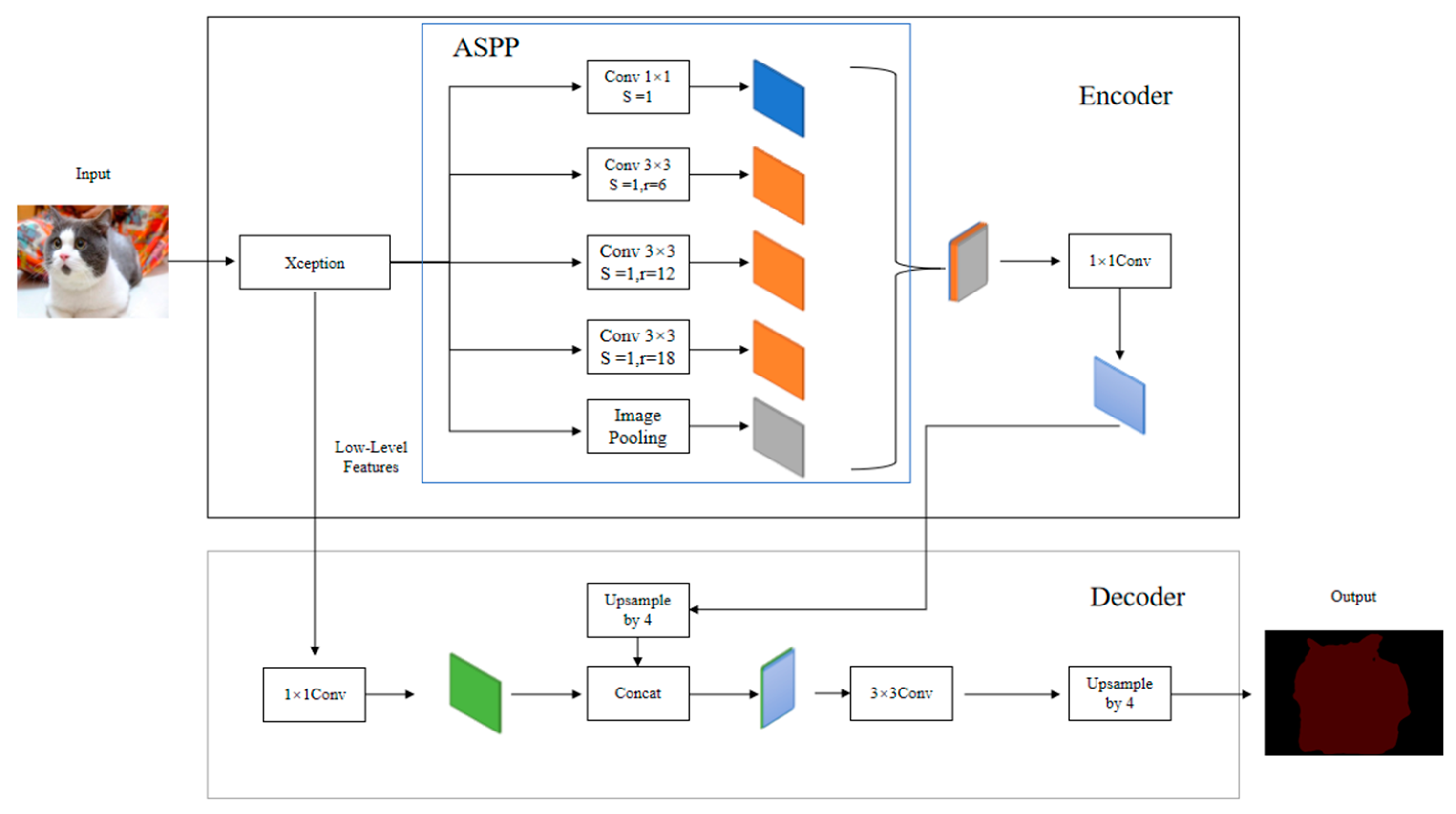
The DeepLabV3+ algorithm can recognize targets in complex environments. The encoder part shown in
Figure 2 is responsible for passing the input information to the Xception backbone for obtaining different levels of feature information. The ASPP module is then utilized for reinforcement learning of the high-level information. In the decoder, the extracted low-level features are first processed to reduce the number of channels. At the same time, the reinforced information output in the encoder is recovered in size, and then the two features are spliced and fed into the 3 × 3 convolution to extract the key information. Then, the feature map is upsampled and enlarged 4 times to obtain the prediction map. In the
Figure 2, Conv denotes convolution. S is the step size, and r is the dilation rate.
After the model segmentation, the model realizes the accurate classification of the beacon spot in the complex background so as to extract the beacon spot target in the image.
Figure 3 shows the effect of using the benchmark DeepLabV3+ model to detect the beacon spot in the interference situation. Its segmentation capability is superior to traditional thresholding segmentation techniques. However, the benchmark model still has errors in the detection of small target light spots under interference and takes a long time, which needs to be further improved.
3. Improvement Measures
3.1. MobileNetV2 Network
When fast target identification is required, the backbone can use MobileNetV2 to speed up model inference. The MobileNet network focuses on the application in microcomputers, and its structure is lightweight and efficient. MobileNetV1 proposes the method of channel-by-channel convolution and then point-by-point convolution to speed up the computation, which is named depthwise separable convolution. The newly proposed MobileNetV2 found that the loss of ReLU in V1 is due to low-dimensional information, and these losses are likely to cause most of the convolution kernels to be 0. So, it adds a linear bottleneck layer between different layers. The model adds inverse residual blocks to better utilize the information. The structure of the V2 version consists of convolutional blocks, inverse residual blocks, and average pooling, and the main layout flow is shown in
Table 1, where
t is the coefficient of expansion,
c is the number of channels,
n denotes the repetition factor of an operation,
denotes the step size when an operation is performed for the first time, and
is 1 for all the repeated portions later on, and m_Out is the number of channels in the model classification output [
20]. Bottleneck denotes the inverse residual module. “—” indicates that the model does not have this operation.
3.2. CBAM Attentional Mechanisms
The benchmark model is not precise in recognizing such tiny objects as beacon spots, and the application of the attention mechanism can realize the precise recognition of beacon spots by focusing on the target features. CBAM is one of the common ones. Its structure is shown in
Figure 4.
![Photonics 11 00451 i001]()
represents the multiplication operation.
Figure 5 shows the steps for realizing channel attention, where Output represents the output channel weights. A pooling operation is performed to remove redundant features. Maxpool denotes maximum pooling, and Avgpool denotes average pooling. The input feature layer passes through a parallel pooling layer and then learns features through a shared fully connected layer (Shared MLP), and then the two outputs are summed pixel by pixel (
), and after Sigmoid function activation, the weights are output.
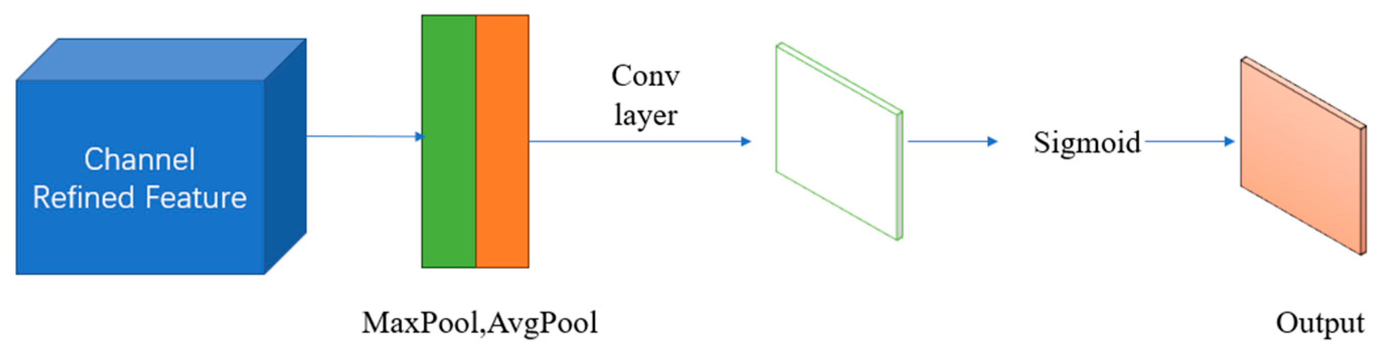
The steps of spatial attention realization are shown in
Figure 6, where Conv layer represents the reduced dimensional convolution. The input features are first subjected to maximum pooling and average pooling, and then the results are spliced. After that, it is subjected to dimensionality reduction, and the activation function is used to obtain a pixel-by-pixel weighted layer.
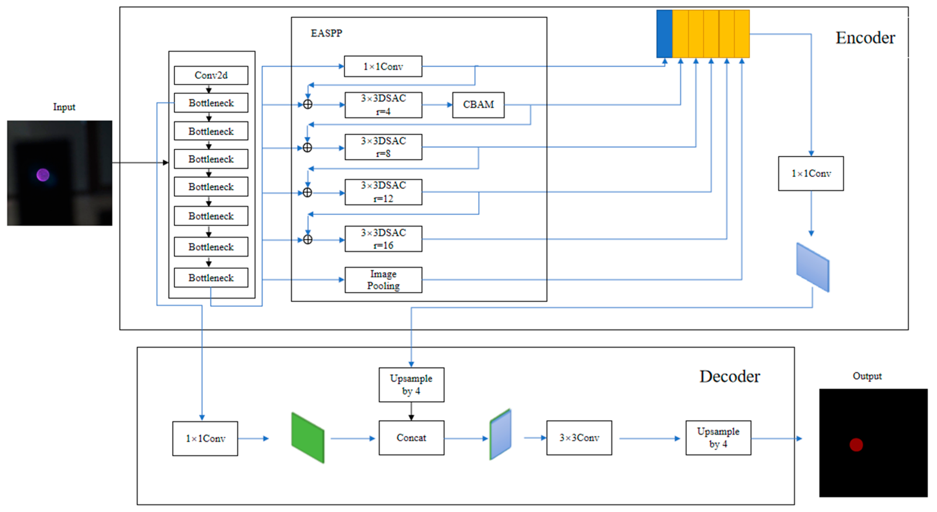
3.3. Improved ASPP Module
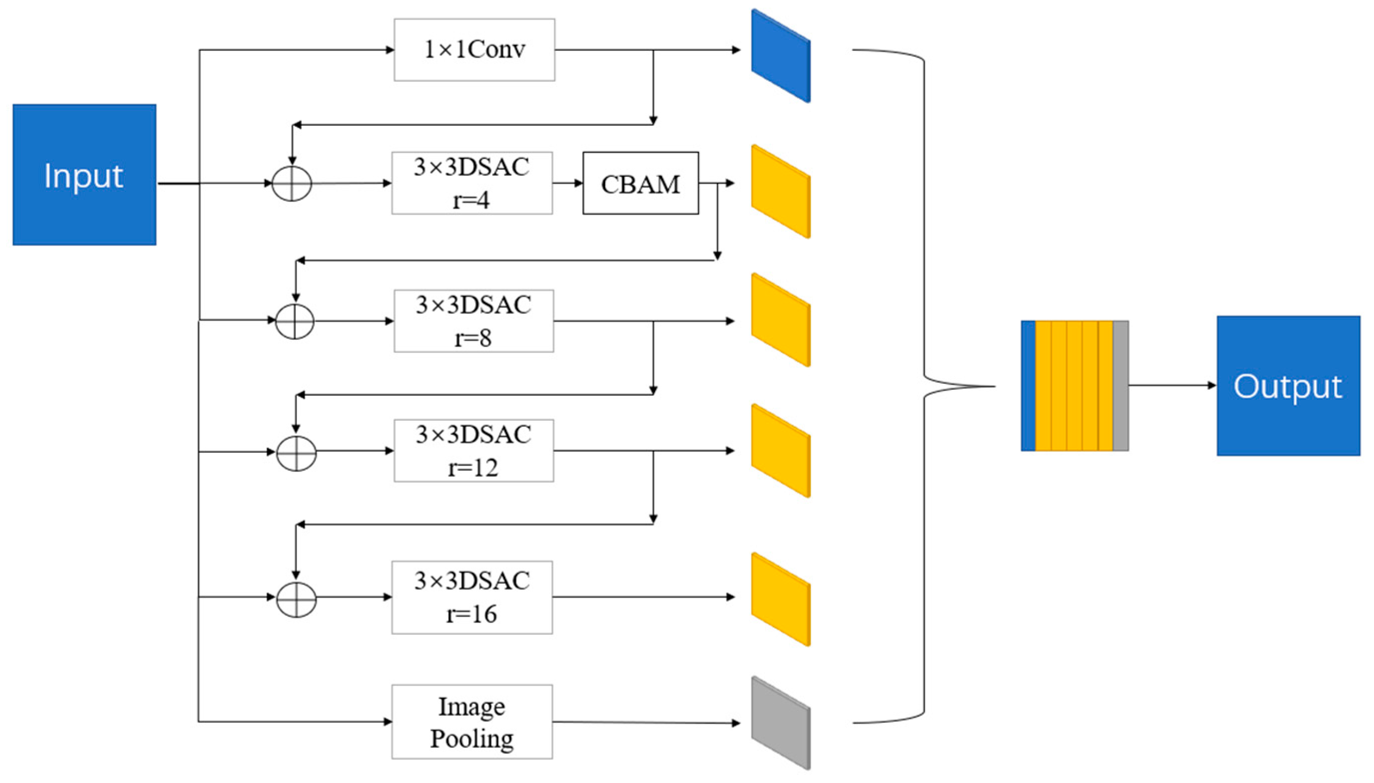
The feature layer in the original ASPP structure after atrous convolution is fused with shallow features to extend the receptive field for model learning. The original convolution in the module is rewritten as a depthwise separable convolution with a dilation rate to reduce the computational burden. And it is named Depthwise Separable Atrous Convolution (DSAC). Compared with the original dilation rate of 6, 12, and 18, since the large step size will damage the extraction of small targets, the dilation rate is adjusted to 4, 8, 12, and 16, and the dilation rate step size is reduced to minimize the features lost to small targets. Meanwhile, in order to make the small target features more accurate and the coordinate information more precise, the CBAM is inserted after the convolution with a dilation rate of 4. The new model is named Efficient ASPP (EASPP), as shown in
Figure 7, where r represents the dilation rate and
represents the fusion on a channel-by-channel basis.
The design of EASPP helps to expand the receptive field, which is the range of pixel points in the feature layer after convolution corresponding to the range of pixel points before convolution [
21]. The method of receptive field calculation is shown as follows:
When
,
where
and
is the value of the convolution kernel,
denotes the number of layers.
refers to the
-th layer receptive field, and
denotes the
+ 1-th layer receptive field.
is the product of the step sizes of all previous layers.
denotes the step value of layer
.
The step value of the original ASPP module is always 1. Equation (3) shows the method for calculating the size of the convolution kernel for an atrous convolution, where
denotes the dilation rate:
DeppLabV3+ has a dilation rate of (6, 12, 18), so the maximal receptive field is
where
and
.
Through the fusion of feature layers, the co-utilization of information between each branch is achieved, and the reinforced feature layers of ASPP also achieve interdependence, which helps to give the model a wider receptive field and can make better use of the input information.
3.4. Focal Loss Function
Conventional models generally choose the cross-entropy loss function with the expression Equation (5):
In the binary classification task, the expression is
is the labeled value, and is the inferred value.
The samples collected in practice are prone to the phenomenon of uneven data distribution, thus impairing the performance of the model. For simple samples, to reduce the proportion of loss weights, the focus loss function can be introduced during training for compensation. The expression of the focal loss function is
where
is the adjustable factor.
This leads to the equation
The coefficients of the focal loss function are . When the sample belongs to the case of easily divisible positive samples , tends to 0. This reduces the proportion of this sample in the loss function at this time. When samples are misclassified, , , at this point, the results do not have much impact on the loss. Thus, the focal loss function can effectively reduce the proportion of simple samples in the loss function, as well as being resistant to misclassified samples.
3.5. Improved Overall Framework
Figure 8 is the model composition diagram of this paper. In the encoder, the input is learned by the backbone and fed into EASPP. EASPP is an augmentation of the original module, which first adjusts the dilation rates to 4, 8, 12, and 16 so that large and small targets have corresponding dilation values. Its inputs and outputs are then spliced together as a way to obtain a larger receptive field. Then, the CBAM is set after the convolutional layer with a dilation rate of 4. This makes the fringe information of the beacon spot more visible. The key information is then integrated to obtain the final effective feature map. In the decoder part, the output of the first time in MobileNetV2 after the inverse residual block is used as the low-level feature information and is subjected to a reduction in the number of channels. The high-level features obtained in the encoder are reduced in size and fused with the low-level features, followed by convolution to adjust the effective features. At the end of the network, the resulting feature image is quadruple-upsampled to output the segmentation result map.
4. Comparison of Training Results and Analysis
4.1. Experimental Environment and Dataset
For this experiment, we chose Ubuntu 20.04 OS, Pytorch framework, and a GeForce RTX 3090 graphics card in order to validate the structure of this network, and we learned the enhanced dataset of PASCAL VOC 2012 [
22] as one of the validation criteria. Secondly, in order to meet the needs of the project, the actual performance was verified by building a light spot dataset.
4.2. Experimental Evaluation Indicators
(mean intersection over union) and
(mean pixel accuracy) are commonly used to evaluate model performance [
23]. Equations (10) and (11) are the calculation formulas:
where
is the number of classes within the dataset, i is the true value, j is the inferred value,
is the number of pixels with both labeled and inferred values of class i, and
is the number of pixels with labeled values of class i and inferred values of class j.
4.3. PASCAL VOC Dataset Comparison Test
The experimental controls mainly include UNet, PSPNet, DeepLabv3+ where the backbone network is MobileNetV2, DeepLabV3+ benchmark network, and the improved model of this study.
Table 2 shows the data for the comparative analysis of content.
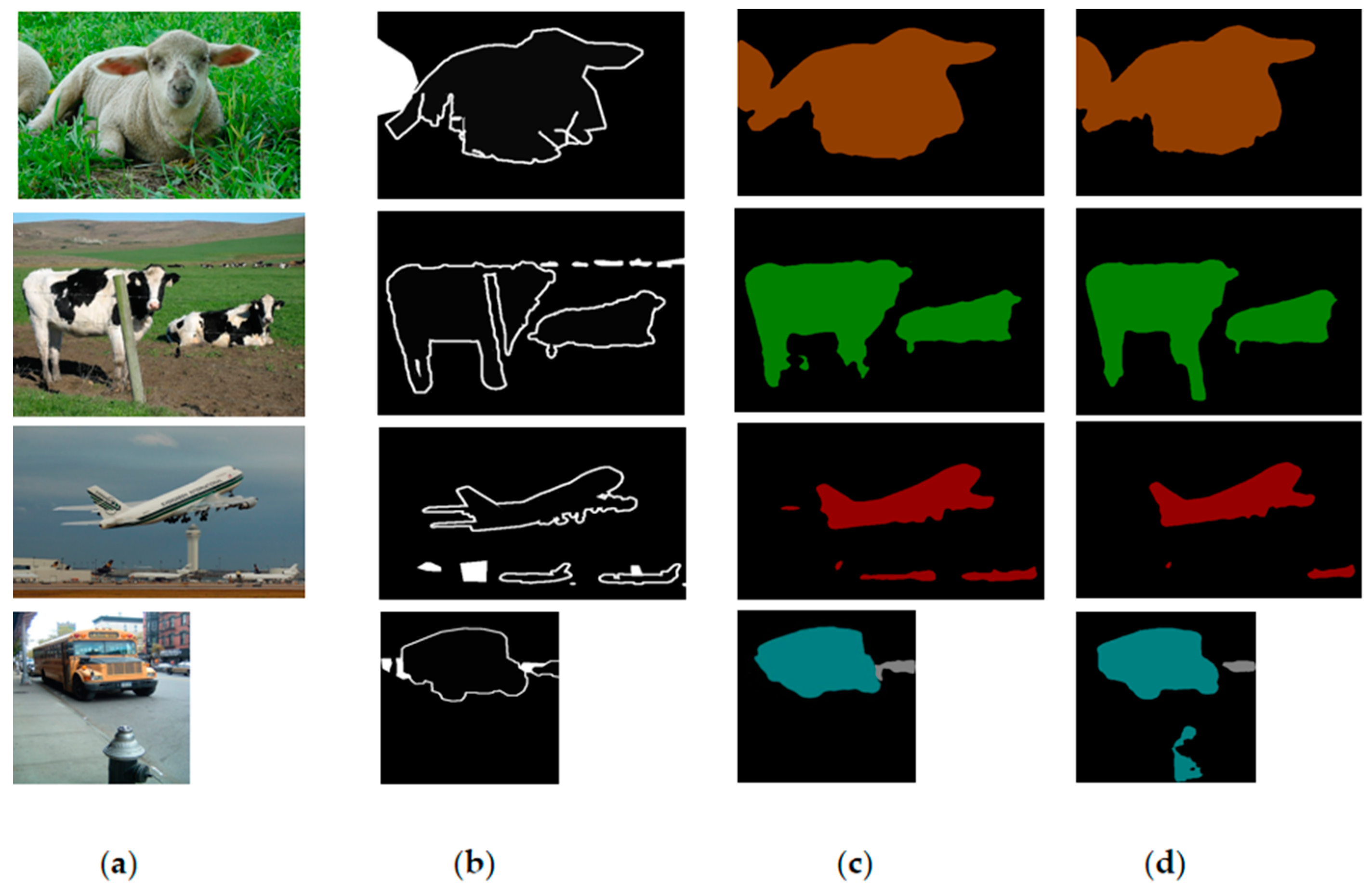
Figure 9 shows the identification of this model against the benchmark model on the dataset.
Table 2 shows that the model in this paper has a lower number of parameters and high segmentation accuracy, although the mIoU is reduced by 2.09 and the MPA is reduced by 2.67 compared to the benchmark model with Xception, but the total number of parameters is reduced to nearly 1/13 of that of the benchmark model. Compared with the fourth group, not only is the number of parameters reduced but also the mIoU and the MPA are improved by 2.25 and 1.76, respectively. PSPnet performs the best, with both mIoU and MPA exceeding those of the other models, but the quantity of parameters is higher than that of the model in this paper, and Unet performs the least effectively.
Figure 9 shows some of the prediction result plots of this paper’s model structure against the benchmark model structure on the PASCAL dataset. On some dataset images, the model in this paper is more accurate than the benchmark model. The fourth row even misclassifies the fire hydrant, while this paper’s model can accurately segment the location of the school bus.
The main reason is that the model in this paper adopts a cascade approach to fuse the contextual semantics, thus broadening the receptive field of model learning. Meanwhile, more dilation rates obtain more information at different scales, and the information is utilized more efficiently. Secondly, in the first row of the figure, the segmentation contour obtained from this paper’s model is more rounded, and the details are more accurate than those of the benchmark model. The comparison result graph proves that this paper’s network pays more attention to the segmented objects and obtains more accurate edge information when segmenting the image.
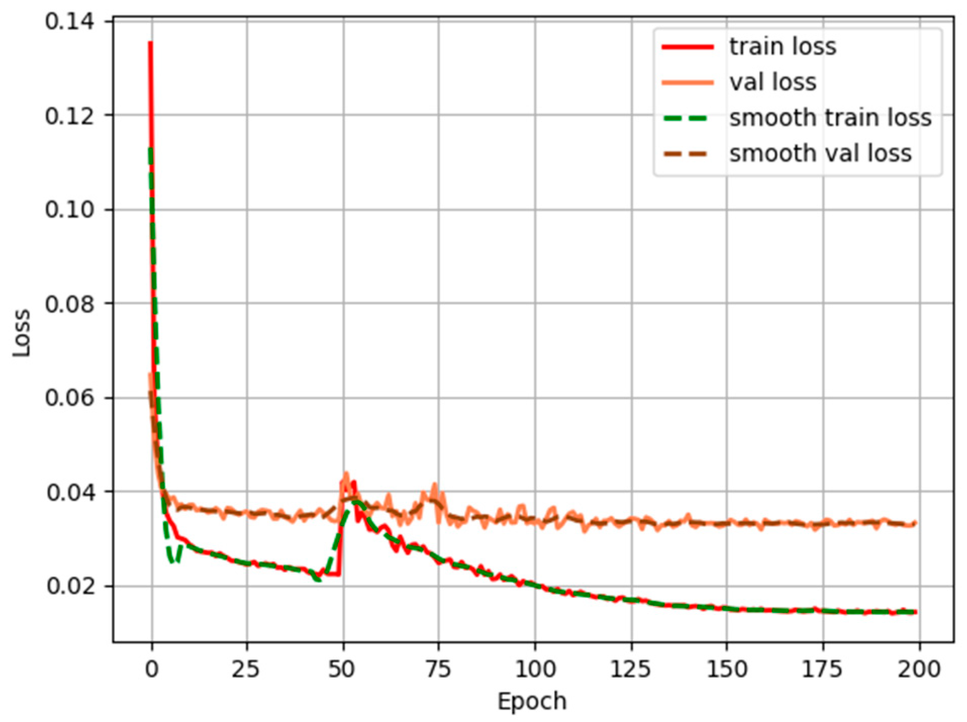
In
Figure 10, although the direction of the loss function fluctuates, it shows a decreasing convergence trend and finally remains stable. The training loss function is finally stable at 0.014, the validation loss function is finally stable at 0.032.
4.4. Beacon Spot Dataset Comparison
A self-constructed beacon spot dataset was used for training the model to recognize targets. An industrial camera was used to capture light spots at different locations with different backgrounds, and a total of 2000 images were collected. The dataset consists of three parts, which are divided according to the standard of 7:2:1, with the training set accounting for seventy percent, the testing set accounting for twenty percent, and the validation set accounting for ten percent. In order to prevent the model from overfitting, the beacon spot dataset images were enhanced and expanded; the image enhancement included the adjustment of brightness and contrast, and the expansion process was mainly ±10° rotation operation on the training set.
Figure 11 illustrates a portion of the beacon spot image.
Several models were selected for the experiment for comparison with the improved model on the light spot dataset, and the data are recorded in
Table 3. The mIoU of this model is 1.33 higher than the benchmark model, and the segmentation time is only nearly one-half of that of the benchmark model. The mIoU is 2.19 higher than that of DeepLabv3+ where the backbone network is MobileNetV2. The mIoU is 1.42 higher compared to the Unet model. The data show that the model in this paper has the strongest ability to recognize beacon spots compared to other models.
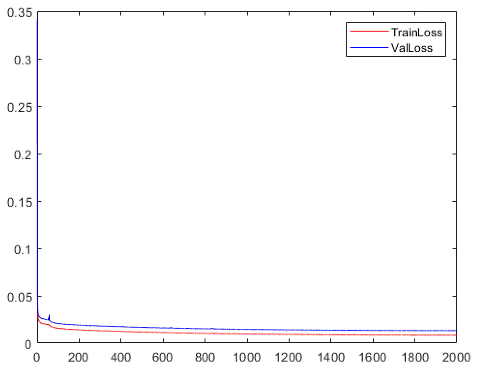
As shown in
Figure 12, the loss value decreases rapidly in the first few rounds and then slowly decreases and stabilizes. In the first round, the loss value is 0.33, and then it keeps decreasing. The validation loss function has small fluctuations but recovers quickly until it finally stabilizes around 0.015. This shows that the model can converge well on the light spot dataset and achieve the stabilization effect.
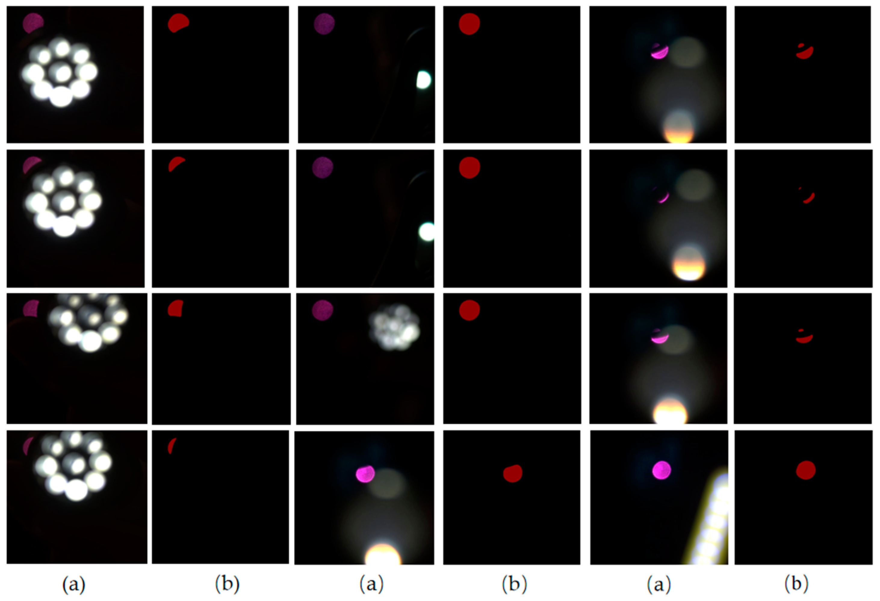
4.5. Beacon Spot Recognition Immunity Test
The reliability of the present algorithm was tested by interfering with the beacon spot using different shapes and intensities of interfering light.
Figure 13 shows part of the experimental segmentation diagram. It can be seen in the figure that in the face of different degrees of interference, even if the beacon spot is blocked, the model can still identify the pixels belonging to the beacon spot and realize high-precision segmentation. This is mainly due to the fact that the EASPP module makes model learning more efficient, and the CBAM allows for more accurate learning of small targets such as beacon spots.
4.6. Ablation Experiment
In order to confirm the usefulness of the EASPP module and the insertion of the CBAM attention module proposed in this paper for model performance enhancement, the conclusions of this paper were verified by comparative ablation experiments with the DeepLabV3+ model whose backbone network is MobileNetV2.
Table 4 shows the different combinations of ablation experiments set up, and
Table 5 records the comparison of experimental data on the PASCAL dataset for the ablation experimental group. In
Table 5, the effect of adding the EASPP module is significant, the mIoU of the model goes up by 1.36, and the MPA goes up by 0.56. The number of model parameters is reduced by 1.606 M, and the segmentation time is reduced by 2 ms. After the CBAM is added on top of Combination ②, the mIoU improves by 0.89, the MPA improves by 1.2, and the number of parameters increases by 0.022 M, but there is almost no effect on the segmentation elapsed time. This suggests that the EASPP module and the introduction of CBAM can effectively reduce the segmentation time and better recognize the target.
4.7. Algorithmic Pseudo-Code
Before the experiment starts, the experimenter sets up the number of times the model will be trained, the batch size, the learning rate, the optimizer, and so on, and then starts the training.
Input: Dataset, initialize network parameter weights.
- (1)
The experiment starts by loading the training dataset and batch parameters and adjusting the learning rate.
- (2)
The experiment will freeze the backbone network MobileNetV2 and train the EASPP feature extraction module of this paper.
- (3)
The loss values are calculated based on the predicted values of the model and the labeled values of the training set.
- (4)
The model begins the backpropagation process, at which point the model is updated based on the gradient of the loss values.
- (5)
The model starts unfreezing training and repeats (3) and (4) until the network finally converges.
- (6)
The model saves the parameters obtained from training.
Output: Trained weights.
5. Discussion and Conclusions
In adaptive optics capture and tracking systems for optical communication, the capture and localization of the beacon spot are essential. Traditional segmentation methods are weak in response to interference, and this paper uses a semantic segmentation algorithm to enhance the reliability when recognizing beacon spots. The algorithm model is DeepLabV3+ and adjusted according to the needs of the project. MobileNetV2 is used as the backbone part of recognizing the beacon spot so as to reduce the number of operations. Next, the ASPP module is adjusted by setting the dilation rate in it to 4, 8, 12, and 16 and splicing the inputs and outputs of the ASPP structure to obtain a larger convolutional receptive field and strengthen the ability to learn the beacon spot features. And the new structure is named EASPP. Then, using CBAM, more attention is paid to the extraction of such small targets as beacon spots, while the DSAC module is utilized to enhance the computing speed, and the focus loss function is introduced into the training so as to improve the performance.
Experimental tests revealed that the improved DeepLabV3+ network achieved mIoU and MPA values of 98.76 and 99.38, respectively, on the spot dataset, with each beacon spot image segmentation taking 12 ms. The improved DeepLabV3+ network achieved mIoU and MPA values of 74.88 and 83.79, respectively, on the enhanced dataset of PASCAL VOC 2012, with each image segmentation taking 10 ms. The number of parameters in the improved model is only 4.234 M, which is close to 1/13 of that of the benchmark model. It is derived from ablation experiments that the EASPP module proposed in this paper reduces the parameters and at the same time effectively improves the model performance. And the inserted CBAM provides an effective performance enhancement with a small computational burden.
We tested a selection of images from the PASCAL dataset, and the improved model has more accurate segmentation results and sharper edge features compared to the baseline model. The model in this paper is able to recognize the beacon spot under the interference environment, whether there is strong light interference or the beacon light is blocked. This is mainly due to the various improvements of the model in this paper, so that the performance of the model has been effectively improved, and more attention can be paid to the segmentation of such small objects as beacon spots. The improved DeepLabV3+ can effectively remove the complex background environment, realize accurate and fast recognition of beacon spots in optical communication, and improve the communication quality.
Applying the algorithms of this paper to practical engineering requires deploying the algorithms to embedded devices. NVIDIA’s Jetson series devices can be selected, and TensorRT technology can be used to realize fast inference on embedded devices to complete the capture and tracking of beacon spots.
Author Contributions
Conceptualization, J.L. and X.N.; data curation, J.L.; formal analysis, J.L. and X.N.; funding acquisition, X.N.; investigation, X.Y. and C.L.; methodology, J.L. and X.N.; project administration, X.N.; resources, X.N. and X.Y.; software, J.L.; supervision, X.N.; validation, J.L. and X.N.; visualization, J.L. and X.N.; writing—original draft, J.L.; writing—review and editing, J.L. and X.N. All authors have read and agreed to the published version of the manuscript.
Funding
National Natural Science Foundation of China Youth Fund Grant Program, grant number 62205032; National Natural Science Foundation of China, grant number 62275033; Science and Technology Research Program of Jilin Provincial Department of Education, grant number JJKH20220749KJ; Jilin Science and Technology Development Program Project, grant number 20210201139GX.
Institutional Review Board Statement
Not applicable.
Informed Consent Statement
Not applicable.
Data Availability Statement
The original contributions presented in the study are included in the article, further inquiries can be directed to the corresponding author.
Conflicts of Interest
The authors declare no conflicts of interest.
Abbreviations
| Abbreviation | Full Name |
| ASPP | Atrous Spatial Pyramid Pooling |
| CBAM | Convolutional Block Attention Module |
| DSAC | Depthwise Separable Atrous Convolution |
| EASPP | Efficient ASPP |
| mIoU | Mean Intersection over Union |
| mPA | Mean Pixel Accuracy |
References
- Farell, T.C. The effect of atmospheric optical turbulence on laser communications systems: Part 1, theory. In Sensors and Systems for Space Applications XII; SPIE: Bellingham, WA, USA, 2019; Volume 11017. [Google Scholar] [CrossRef]
- Xing, J.B.; Xu, G.L.; Zhang, X.P. Effect of the atmospheric turbulence on laser communication system. Acta Photonica Sin. 2005, 34, 1850–1852. [Google Scholar]
- Chen, M. Research on Key Technology of Star-Ground Laser Communication Ground Station Based on Large Aperture Telescope. Ph.D. Thesis, University of Chinese Academy of Sciences (Institute of Optoelectronic Technology, Chinese Academy of Sciences), Beijing, China, 2019. [Google Scholar]
- Wang, B.F. Research on Laser Precision Tracking Technology Based on Adaptive Optics. Master’s Thesis, Graduate School of Chinese Academy of Sciences (Xi’an Institute of Optical Precision Machinery), Xi’an, China, 2015. [Google Scholar]
- Fu, J.H.; Wang, J.P.; Wen, L.H.; Shi, Z.Z. Brightfield stem cell image segmentation method based on improved threshold and edge gradient. Electron. Meas. Technol. 2020, 43, 109–114. [Google Scholar]
- Shi, H.D.; Hou, J.; Chen, M.J.; Yi, J.; Hu, J. Improved Segmentation Method of DeepLabv3+ Face Mask. Radio Eng. 2023, 53, 957–967. [Google Scholar]
- Girshick, R. Fast R-CNN. In Proceedings of the 2015 IEEE International Conference on Computer Vision, Santiago, Chile, 7–13 December 2015; IEEE Press: New York, NY, USA, 2015; pp. 1440–1448. [Google Scholar]
- Long, J.; Shelhamer, E.; Darrell, T. Fully Convolutional Networks for Semantic Segmentation. In Proceedings of the 2015 IEEE Conference on Computer Vision and Pattern Recognition, Boston, MA, USA, 7–12 June 2015; pp. 3431–3440. [Google Scholar]
- Ronneberger, O.; Fischer, P.; Brox, T. U-Net: Convolutional Networks for Biomedical Image Segmentation. In Proceedings of the International Conference on Medical Image Computing and Computer-Assisted Intervention, Munich, Germany, 5–9 October 2015; pp. 234–241. [Google Scholar]
- Badrinarayanan, V.; Kendall, A.; Cipolla, R. SegNet: A Deep Convolutional Encoder-Decoder Architecture for Image Segmentation. IEEE Trans. Pattern Anal. Mach. Intell. 2017, 39, 2481–2495. [Google Scholar] [PubMed]
- Zhao, H.; Shi, J.; Qi, X.; Wang, X.; Jia, J. Pyramid Scene Parsing Network. In Proceedings of the 2017 IEEE Conference on Computer Vision and Pattern Recognition, Honolulu, HI, USA, 21–26 July 2017; pp. 2881–2890. [Google Scholar]
- Chen, L.C.; Papandreou, G.; Kokkinos, I.; Murphy, K.; Yuille, A.L. Semantic Image Segmentation with Deep Convolutional Nets and Fully Connected CRFs. arXiv 2014, arXiv:1412.7062. [Google Scholar]
- Chen, L.C.; Papandreou, G.; Kokkinos, I.; Murphy, K.; Yuille, A.L. DeepLab: Semantic Image Segmentation with Deep Convolutional Nets, Atrous Convolution, and Fully Connected CRFs. IEEE Trans. Pattern Anal. Mach. Intell. 2017, 40, 834–848. [Google Scholar] [PubMed]
- Chen, L.C.; Papandreou, G.; Schroff, F.; Adam, H. Rethinking Atrous Convolution for Semantic Image Segmentation. arXiv 2017, arXiv:1706.05587. [Google Scholar]
- Chen, L.C.; Zhu, Y.; Papandreou, G.; Schroff, F.; Adam, H. Encoder-Decoder with Atrous Separable Convolution for Semantic Image Segmentation. In Proceedings of the 2018 European Conference on Computer Vision (ECCV), Munich, Germany, 8–14 September 2018; pp. 801–818. [Google Scholar]
- Chollet, F. Xception: Deep Learning with Depthwise Separable Convolutions. In Proceedings of the 2017 IEEE Conference on Computer Vision and Pattern Recognition, Honolulu, HI, USA, 21–26 July 2017; pp. 1251–1258. [Google Scholar]
- Woo, S.; Park, J.; Lee, J.Y.; Kweon, I.S. CBAM: Convolutional Block Attention Module. In Proceedings of the 2018 European Conference on Computer Vision (ECCV), Munich, Germany, 8–14 September 2018; pp. 3–19. [Google Scholar]
- Sandler, M.; Howard, A.; Zhu, M.; Zhmoginov, A.; Chen, L.C. MobileNetV2: Inverted Residuals and Linear Bottlenecks. In Proceedings of the 2018 IEEE Conference on Computer Vision and Pattern Recognition, Salt Lake City, UT, USA, 18–23 June 2018; pp. 4510–4520. [Google Scholar]
- Lin, T.Y.; Goyal, P.; Girshick, R.; He, K.; Dollár, P. Focal Loss for Dense Object Detection. In Proceedings of the 2017 IEEE International Conference on Computer Vision, Venice, Italy, 22–29 October 2017; pp. 2980–2988. [Google Scholar]
- Gong, K.; Cheng, Y.H.; Hou, F.F.; Fan, X.Y.; Wang, Y.J. Pedestrian and vehicle detection algorithm based on Mobilenetv2-YOLOv4 model. Comput. Inf. Technol. 2023, 31, 1–5+37. [Google Scholar]
- Zhou, Y.; Pei, S.H.; Cheng, H.Y.; Yan, Y.Z. A defect generation algorithm for solar cells combining multiple receptive fields and attention. Pattern Recognit. Artif. Intell. 2023, 36, 366–379. [Google Scholar]
- Xu, W.; Wang, H.; Qi, F.; Lu, C. Explicit Shape Encoding for Real-time Instance Segmentation. In Proceedings of the 2019 IEEE/CVF International Conference on Computer Vision, Seoul, Republic of Korea, 27 October–2 November 2019; pp. 5168–5177. [Google Scholar]
- Xie, G.B.; He, L.; Lin, Z.Y.; Zhang, W.L.; Chen, Y. Lightweight optical remote sensing image road extraction based on L-DeepLabv3+. Laser J. 2024, 45, 111–117. Available online: http://kns.cnki.net/kcms/detail/50.1085.TN.20230529.1620.004.html (accessed on 2 May 2024).
| Disclaimer/Publisher’s Note: The statements, opinions and data contained in all publications are solely those of the individual author(s) and contributor(s) and not of MDPI and/or the editor(s). MDPI and/or the editor(s) disclaim responsibility for any injury to people or property resulting from any ideas, methods, instructions or products referred to in the content. |
© 2024 by the authors. Licensee MDPI, Basel, Switzerland. This article is an open access article distributed under the terms and conditions of the Creative Commons Attribution (CC BY) license (https://creativecommons.org/licenses/by/4.0/).


 represents the multiplication operation.
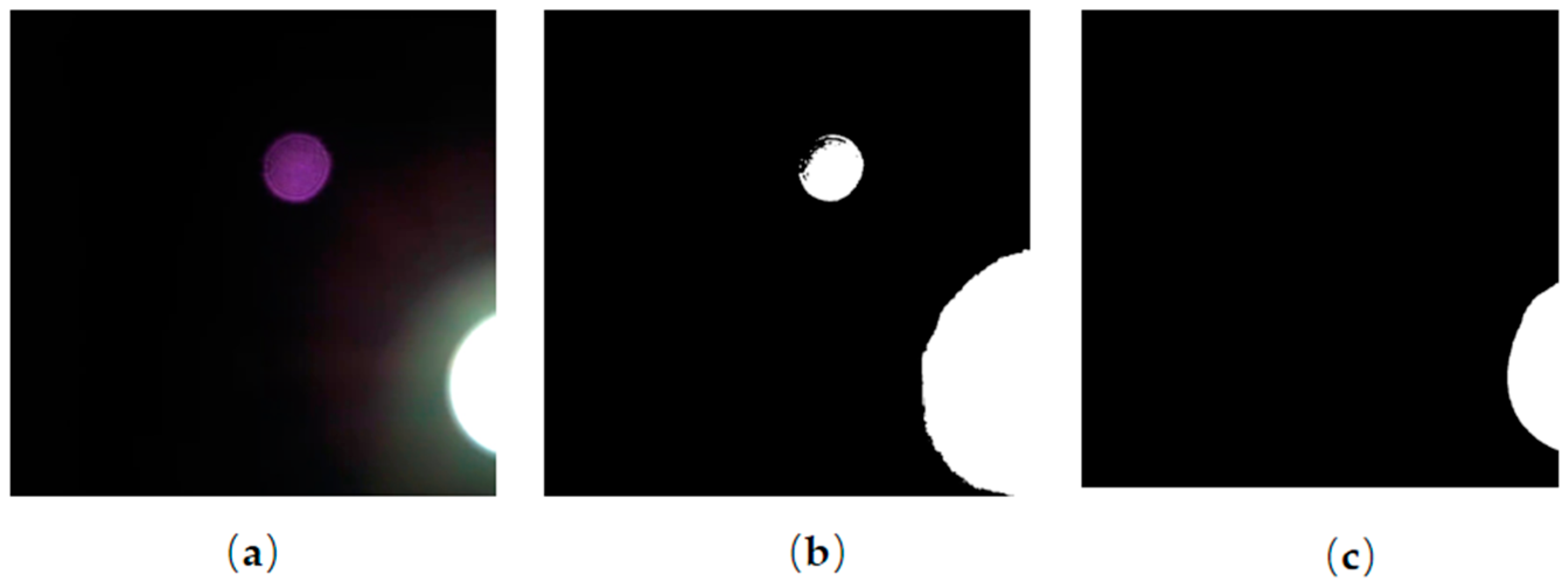


