Weak Value Amplification of Photons in Optical Nonlinear Medium, Opto-Mechanical, and Spin-Mechanical Systems

Abstract

A measurement of an observable A performed on a quantum system that is initially prepared in a state ${\rho }_i$, followed by a probabilistic procedure that leaves the system in a final state ${\rho }_f$, a process often referred as state postselection (or filtering process), can yield, on average, anomalous measurement results, i.e., values that may exceed the eigenvalue range of the observable being measured or be complex numbers. There is, therefore, an amplification effect of the average measurement result, i.e., the effect of the system on the measurement device is increased. When the coupling between the system and the measurement device satisfies some weakness conditions, the amplification effect occurs due to the weak value of the operator A. In this article, the amplification effect due to the postselection process is reviewed, and theoretical proposals and experiments published in the recent literature on the field are commented on. The emphasis is made on interactions occurring in optical nonlinear media and opto-mechanical and spin-mechanical systems, in which the amplification of number operators takes place.

1. Introduction

The weak values of an observable were introduced by Aharanov, Albert, and Vaidman in 1988 [1]. In general, weak values are complex numbers that appear when the outcomes of independent repetitions of an experiment are averaged. In order for weak values to emerge, the experiments should include two key ingredients: weak measurements (weak interactions between the measurement apparatus and the measured system) and postselection (a certain class of filtering process). In this operational or statistical sense, weak values are analogous to expectation values. However, they may be complex quantities or lie outside the eigenvalue range of the observable, in which case the weak values are said to be anomalous. In these situations, the effect of the measured system on the measurement apparatus is therefore amplified, which is often referred to as weak value amplification.

This effect has been used in metrology for the estimation of small effects such as beam deflections [2], frequency shifts [3], phase shifts [4], Doppler shifts [5], longitudinal phase shifts [6], angular rotations [7] or temperature shifts [8]. Possibly, one of the first applications of weak values in precision metrology was the observation of the Spin Hall effect of light, where a beam displacement in the order of angstroms was detected [9]. Similarly, in an experiment performed by Dixon, Starling, Jordan, and Howell [10], a tilted mirror (controlled by a piezoelectric actuator) produces a displacement of the transverse position of a light beam of the order of μm. Attenuating the light beam, from an initial intensity in the range of mW down to $10-{10}^2$μW, by means of a Sagnac interferometer and analyzing only the output light at one of the exit ports of the interferometer (a nearly dark port), the displacement was enlarged by factors of over 100. The amplification effect enabled the measurement of the angular displacement of the mirror down to 400 pm, therefore allowing for the indirect measurement of the linear travel of the piezo actuator, which was on the order of fm (comparable to the radius of a single proton).

From a more fundamental perspective, and given that a weak measurement barely perturbs the system under observation, weak values have been useful to analyze quantum experiments that lead to paradoxes when analyzed in a counterfactual manner [11,12,13].

In this article, we will review experimental verifications of weak value amplification and theoretical proposals in which the amplified variable corresponds to a photon number operator. When the weak value of such an operator is anomalous, the effect of the photons on the measurement device is amplified or enlarged, i.e., “a few photons” may behave as “many photons” do (at least, with regard to their effect on the measurement apparatus). Additionally, when the experiment is based on single photons, the number operator may be regarded as a projection operator in the single photon subspace. Since the expectation value of a projector corresponds to the probability of reading the +1 eigenvalue of the projector, an anomalous weak value of a projector may be considered to be negative (or complex) probability [14]. On the other hand, weak values can be expressed as the expectation value under a quasi-probability distribution, called the (extended) Kirkwood-Dirac distribution [15]. It has been proven that negative values of the Kirkwood-Dirac distribution have metrological advantages as compared to classical protocols [16]. Therefore, the amplification of number operators is of both practical and fundamental interest.

This article is structured as follows. In Section 2, the weak value amplification effect and, in general, amplification by postselection is described. As was pointed out previously, weak values emerge when weak measurements are combined with a procedure called postselection. All these aspects are commented on in the first section. Then, in Section 3, a nonlinear quantum optics experiment is described, in which an anomalous weak value of a photonic number operator allows the enlargement of the phase imprinted by a single photon on a classical beam. Then, in Section 4 and Section 5, an experiment and theoretical proposals on the amplification of number operators via weak values or postselection in opto-mechanical and spin-mechanical systems are commented. Finally, in Section 6, the main ideas described in the article are summarized, and further discussion of metrological aspects is included.

2. Weak Value Amplification Effect

The “play” takes place in a “measurement scenario”, in which two particles take part. One particle is the measurement device, or meter (M), that interacts with a system (S). Then, some meter variable is observed in order to gain information about the system. Both particles are described quantum mechanically, i.e., there is one Hilbert space associated with the system, ${\mathcal{H}}_S$, and another space associated with the measurement device, ${\mathcal{H}}_M$. The total Hilbert space is the tensor product space ${\mathcal{H}}_{SM}={\mathcal{H}}_S\otimes {\mathcal{H}}_M$. In many experiments, both “particles” are different degrees of freedom of the same particle. In other experiments, they are indeed two distinct particles.

Let the free evolution of the system and the meter be dictated by the Hamiltonians $H_S$ and $H_M$, respectively. During the measurement, both particles interact through a Hamiltonian, $H_{SM}$. The total Hamiltonian is, therefore, $H=H_S+H_M+H_{SM}$. It will be assumed that the measurement will be a measurement of a system observable, $A_S$, and that information about this variable will be gained by the observation of a meter variable, $R_M$. For example, in the standard Stern-Gerlach experiment, $A_S$ represents the spin along the z-direction of an atom (the measured observable), while $R_M$ represents the momentum of the atom in the z direction (the variable of the measurement device that allows the gaining of information about the spin). These operators have spectral representations

$$\begin{array}{c}\hfill A_S=\sum _{a\in \mathrm{Spec}\left(A_S\right)}a|a\rangle \langle a|\mathrm{and}{R}_M=\sum _{r\in \mathrm{Spec}\left(R_M\right)}r|r\rangle \langle r|,\end{array}$$

(1)

where $\mathrm{Spec}(★)$ denotes the spectrum of the operator ★. If one of the variables has a continuous spectrum, then the sum should be replaced by an integral. When it is needed for better clarity, subscripts S and M will be used to label system and meter states and observables, respectively. However, when it is obvious, the subscripts will be omitted to avoid too heavy notations.

In general, the measurement device starts in a pure state ${|\psi \rangle }_M$, and the system in a mixed state ${\rho }_S$, i.e., the initial joint state of the system and the measurement device will be a product state ${|\psi \rangle }_M{\langle \psi |}_M\otimes {\rho }_S$. Expectation values computed over the initial state of the measurement device, which, as has been already pointed out, is initially uncorrelated with the system, will be denoted with the subscript i. For example, ${\langle R_M\rangle }_i\equiv {\langle \psi |}_M{R}_M{|\psi \rangle }_M$. Of course, such expectation values depend only on the features of the meter and provide no information about the system.

The standard measurement scheme considered here will be the so-called von Neumann protocol for measurements [17,18]. In this scheme, the interaction Hamiltonian is $H_{SM}=g\delta \left(t\right)A_S{O}_M$, where $O_M$ is some meter variable that couples to the system variable $A_S$ during the measurement. For example, in a measurement of the spin of an atom (along the z-direction), $O_M$ is the transverse position of the atom (in the z-direction). The function $\delta \left(t\right)$ is a Dirac delta function, centered at time $t=0$, that represents the instant at which the measurement takes place. The parameter g is the strength of the coupling between the system and the measurement device. Since the measurement is instantaneous, the effect of $H_S$ and $H_M$ can be neglected, and the evolution operator that describes the measurement process is $U=\exp \{-ig{A}_S{O}_M\}$.

Consequently, the joint state of the system and the meter evolves from the initial product state, before the measurement, to the (in general) entangled state $U{|\psi \rangle }_M{\rho }_S{\langle \psi |}_M{U}^{†}$, after the measurement. When the meter variable $R_M$ is observed and the result r is obtained, the system disentangles from the meter, evolving to the un-normalized conditional state

$$\begin{array}{c}\hfill {\tilde{\rho }}_S{|}_r={\langle r|}_{M}U{|\psi \rangle }_M{\rho }_S{\langle \psi |}_M{U}^{†}{|r\rangle }_M,\forall r\in \mathrm{Spec}\left(R_M\right).\end{array}$$

(2)

The operators ${\langle r|}_{M}U{|\psi \rangle }_M$ are called measurement operators, and will be denoted as $M_r$. Thus, the state ${\tilde{\rho }}_S{|}_r$ can be compactly written as $M_r{\rho }_S{M}_r^{†}$. The norm of this state, $\mathrm{Tr}{M}_r^{†}{M}_r{\rho }_S$, represents the probability to read the result r, which will be denoted as $P\left(r\right)$. The operators $E_r=M_r^{†}{M}_r$ are positive operators that resolve the unity, i.e., ${\sum }_r{M}_r^{†}{M}_r={\mathbb{1}}_S$, defining a positive operator valued measure (POVM). The operators $E_r$ are called probability operators or effects [19].

The unconditional system state after the measurement, i.e., the state after averaging over all possible measurement results, is

$$\begin{array}{c}\hfill {\rho }_{S,\mathrm{un}}=\sum _r{M}_r{\rho }_S{M}_r^{†}.\end{array}$$

(3)

The ensemble average of the measurement results (r), computed under the distribution $P\left(r\right)=\mathrm{Tr}\{M_r^{†}{M}_r{\rho }_S\}$, is given by

$$\begin{array}{c}\hfill {\langle R_M\rangle }_f\equiv \sum _{r\in \mathrm{Spec}\left(R_M\right)}rP\left(r\right)=\mathrm{Tr}\{{\langle \psi |}_M{e}^{ig{A}_S{O}_M}{R}_M{e}^{-ig{A}_S{O}_M}{|\psi \rangle }_M{\rho }_S\}.\end{array}$$

(4)

In a weak measurement, the coupling strength between the system and the meter is weak enough to expand the measurement operators to first order with respect to g,

$$\begin{array}{c}\hfill M_r\equiv {\langle r|}_{M}U{|\psi \rangle }_M\approx \langle r||\psi \rangle {\mathbb{1}}_S-ig\langle r|O_M|\psi \rangle A_S,\forall r\in \mathrm{Spec}\left(R_M\right).\end{array}$$

(5)

In this regime, the unconditional system state (3) can be expressed as

$$\begin{array}{c}\hfill {\rho }_{S,\mathrm{un}}\approx {\rho }_S+ig{\langle O_M\rangle }_i[{\rho }_S,A_S],\end{array}$$

(6)

while the ensemble average of the measurement results (4) becomes

$$\begin{array}{ccc}\hfill {\langle R_M\rangle }_f& \approx & {\langle R_M\rangle }_i+ig{\langle [O_M,R_M]\rangle }_i\mathrm{Tr}\left\{A_S{\rho }_S\right\}.\hfill \end{array}$$

(7)

Expression (6) shows that after the weak measurement, on average, the system is barely perturbed. Moreover, it may remain (on average) unperturbed every time ${\langle O_M\rangle }_i=0$, or when the initial system state commutes with the observable being measured. On the other hand, expression (7) shows that, although the system may remain unperturbed after the measurement, there is still some information about the system that may be gathered by observing $R_M$ (as long as this variable does not commute with $O_M$).

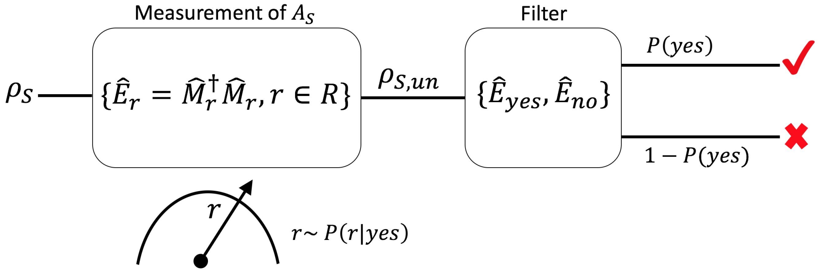
Now, suppose that a filtering process is immediately applied after the measurement (i.e., it will be assumed that the system does not evolve between the measurement and the filtering process). In our context, a filter is a (second) quantum measurement with two outputs: the “yes answer” occurs when the particle passes through the filter, and the “no answer” in the opposite case. In this last scenario, the particles are discarded. Therefore, after the filtering process, the size of an ensemble will be reduced. The effects of the filter will be denoted as $E_{yes}$ and $E_{no}$, and satisfy the completeness relation $E_{yes}+E_{no}=\mathbb{1}$. The first measurement, followed by the filtering process, is illustrated in Figure 1.

Figure 1. A quantum system in an initial state ${\rho }_S$ is subjected to a measurement of the observable $A_S$. The measurement is described by a set of effects $E_r$. In a single instance, the measurement produces an outcome r, a random variable that distributes according to $P\left(r\right)\equiv \mathrm{Tr}\left\{E_r{\rho }_S\right\}$. Then, the system is subjected to the action of a filter, a second quantum measurement with two outcomes: “yes” and “no”. The idea is to consider $r|yes$, i.e., the results of the first measurement conditioning on the successful operation of the filter, a random variable that distributes according to (10).

Figure 1. A quantum system in an initial state ${\rho }_S$ is subjected to a measurement of the observable $A_S$. The measurement is described by a set of effects $E_r$. In a single instance, the measurement produces an outcome r, a random variable that distributes according to $P\left(r\right)\equiv \mathrm{Tr}\left\{E_r{\rho }_S\right\}$. Then, the system is subjected to the action of a filter, a second quantum measurement with two outcomes: “yes” and “no”. The idea is to consider $r|yes$, i.e., the results of the first measurement conditioning on the successful operation of the filter, a random variable that distributes according to (10).

The probability of a particle successfully passing through the filter is

$$\begin{array}{c}\hfill P\left(yes\right)=\mathrm{Tr}\left\{E_{yes}{\rho }_{S,\mathrm{un}}\right\}=\mathrm{Tr}\left\{{\langle \psi |}_M{e}^{ig{A}_S{O}_M}{E}_{yes}{e}^{-ig{A}_S{O}_M}{|\psi \rangle }_M{\rho }_S\right\},\end{array}$$

(8)

while the probability that the filter fails is $1-P\left(yes\right)$. On the other hand, the joint probability to read the value r in the first measurement and then to successfully filter the particle is

$$\begin{array}{c}\hfill P(r,yes)=\mathrm{Tr}\left\{E_{yes}{M}_r{\rho }_S{M}_r^{†}\right\}.\end{array}$$

(9)

The probability of observing the value r in the initial measurement, given that the filter has been successful, can be derived by applying the rule for conditional probabilities,

$$\begin{array}{c}\hfill P(r|yes)=\frac{P(r,yes)}{P\left(yes\right)}.\end{array}$$

(10)

The ensemble average of the measurement results, computed under the conditional distribution $P(r|yes)$, is

$$\begin{array}{c}\hfill {\langle R_M\rangle }_f{|}_{yes}\equiv \sum _{r\in \mathrm{Spec}\left(R_M\right)}rP(r|yes)=\frac{\mathrm{Tr}\left\{{\langle \psi |}_M{e}^{ig{A}_S{O}_M}(E_{yes}\otimes R_M)e^{-ig{A}_S{O}_M}{|\psi \rangle }_M{\rho }_S\right\}}{\mathrm{Tr}\left\{{\langle \psi |}_M{e}^{ig{A}_S{O}_M}{E}_{yes}{e}^{-ig{A}_S{O}_M}{|\psi \rangle }_M{\rho }_S\right\}}.\end{array}$$

(11)

This expression should be compared with expression (4), the average measurement result without applying the filter. Please note that both the numerator and denominator depend on the coupling constant g. Expanding the expression up to the first order with respect to g gives the average result of a weak measurement followed by a filtering process,

$$\begin{array}{c}\hfill {\langle R_M\rangle }_f{|}_{yes}\approx {\langle R_M\rangle }_i+ig{\langle [O_M,R_M]\rangle }_i\mathcal{R}+2g\mathrm{Cov}(O_M,R_M)\mathcal{I},\end{array}$$

(12)

where $\mathrm{Cov}(O_M,R_M)={\langle \{O_M,R_M\}\rangle }_i/2-{\langle R_M\rangle }_i{\langle O_M\rangle }_i$ is the covariance between the apparatus variable $R_M$ and $O_M$, while $\mathcal{R}$ and $\mathcal{I}$ are real numbers defined as

$$\begin{array}{c}\hfill \mathcal{R}=\frac{\mathrm{Tr}(\{E_{yes},A_S\}{\rho }_S)}{2\mathrm{Tr}{E}_{yes}{\rho }_S},\mathcal{I}=\frac{\mathrm{Tr}([E_{yes},A_S]{\rho }_S)}{2i\mathrm{Tr}{E}_{yes}{\rho }_S}.\end{array}$$

(13)

As will be seen in the next sections, in general, the first-order expansion of expression (11) requires that $g\ll \delta$ or $g\ll \epsilon$. The parameter $\delta$ is some parameter associated with the extraction of information, i.e., condition $g\ll \delta$ “allows” a first-order expansion of the positive part of the measurement operator and will be responsible for the term that depends on $\mathcal{R}$. On the other hand, the parameter $\epsilon$ is associated with the measurement back-action (the application of forces that produce random changes in variables that do not commute with $A_S$), i.e., $g\ll \delta$ enables a first-order expansion of the unitary part of the measurement operator and is responsible for the term that contains $\mathcal{I}$. Therefore, the term $\mathcal{R}$ is associated with the extraction of information and $\mathcal{I}$ to the measurement back-action effect [20].

When $E_{yes}=|f\rangle \langle f|$ is a rank one projector into the space spanned by the (normalized) vector $|f\rangle$, and the initial system state is a pure state ${\rho }_S=|i\rangle \langle i|$, then $\mathcal{R}$ and $\mathcal{I}$ become, respectively, the real and imaginary parts of the weak value of $A_S$, defined as

$$\begin{array}{c}\hfill A_w=\frac{\langle f|A_S|i\rangle }{\langle f||i\rangle }.\end{array}$$

(14)

In this case, the average shift of the “meter needle”, ${\langle R_M\rangle }_f{|}_{yes}-{\langle R_M\rangle }_i$, depends on the real and imaginary parts of the weak value; $ig{\langle [O_M,R_M]\rangle }_{i}Re\left(A_w\right)+2g\mathrm{Cov}(O_M,R_M)Im\left(A_w\right)$, a result that was derived by Jozsa [21].

Expression (12) should be compared to (7), where the average shift is proportional to the average value of $A_S$. Now, with the use of a filter, the shift can be enlarged since $\mathcal{R}$ and $\mathcal{I}$ can lie outside the eigenvalue range of $A_S$. There will be, therefore, an amplification effect due to the filtering. For example, if $A_S$ is a number operator, then the effect of the system on the measurement device can be amplified as if the system was made up of “more particles” than the ones that actually are in ${\rho }_S$.

3. Amplification of Photons in a Kerr Medium

The concepts introduced in the previous section are now employed to describe an experiment made by Hallaji, Feizpour, Dmochoswski, Sinclair, and Steinberg (HFDSS) in 2017 [22]. The experiment is based on a theoretical proposal made by Feizpour, Xing, and Steinberg (FXS) in 2011 [23]. First, the theoretical proposal is described, followed by comments regarding the experiment.

The system begins in a pure quantum state with a definite number of photons, $N=1$ (single photon state),

$$\begin{array}{c}\hfill {\rho }_S=|i\rangle \langle i|,|i\rangle =\frac{1}{\sqrt{2}}({|1\rangle }_1{|0\rangle }_2-{|0\rangle }_1{|1\rangle }_2).\end{array}$$

(15)

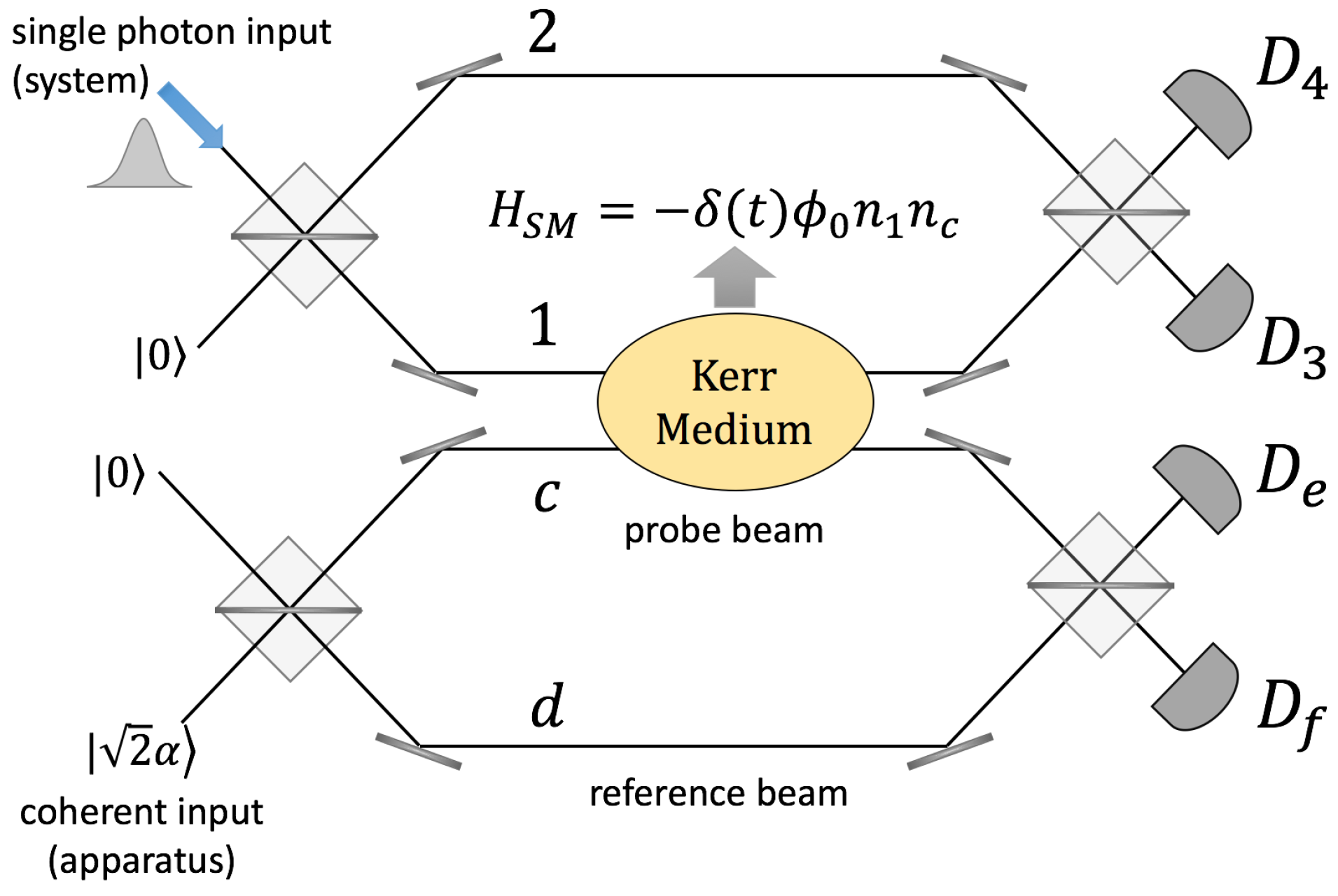
Modes 1 and 2 are propagation modes along paths 1 and 2 of the interferometer, as shown in the upper interferometer of Figure 2. This superposition of modes, or path-entangled state, is prepared by sending a single photon across a 50–50 beam splitter at the entry of the interferometer (while the other input port is in the vacuum state). Only one mode of the system interacts with a coherent beam, which propagates along the arm c of a second interferometer (lower interferometer in Figure 2). The nonlinear interaction between the beam and the single photon occurs in a Kerr medium and is described by the unitary operator $U={\exp }^{i{\varphi }_0{n}_1{n}_c}$. The parameter ${\varphi }_0\ll 1$ is the phase shift generated by a single photon on the probe beam, while $n_1$ is the number operator for mode 1 (a system variable) and $n_c$ the number of photons in mode c (an apparatus variable). In Figure 2, one can note that there is also a reference beam that propagates along arm d of the second interferometer. This beam does not interact with the system and allows the extraction of the phase shift by reading the difference of photons at detectors $D_e$ and $D_f$. Consequently, the “measurement device” has a two-mode structure and is initially prepared in the pure state

$$\begin{array}{c}\hfill {|\psi \rangle }_M={|\alpha \rangle }_c{|i\alpha e^{i\theta }\rangle }_d.\end{array}$$

(16)

Figure 2. Description of the experiment performed by HFDSS [22,23]. The upper interferometer is associated with the system (a single photon), while the lower interferometer is associated with the measurement device. Both the system and the measurement device have a two-mode structure. Modes 1 and c interact in a Kerr medium. Detectors $D_3$ and $D_4$ are used to post-select a final system state, while detectors $D_e$ and $D_f$ are used to read the phase generated on the classical beam. Note: this figure was completely redrawn by the authors of this article, taking Figure 1 of [23] and Figure 1 of [22] as references.

Figure 2. Description of the experiment performed by HFDSS [22,23]. The upper interferometer is associated with the system (a single photon), while the lower interferometer is associated with the measurement device. Both the system and the measurement device have a two-mode structure. Modes 1 and c interact in a Kerr medium. Detectors $D_3$ and $D_4$ are used to post-select a final system state, while detectors $D_e$ and $D_f$ are used to read the phase generated on the classical beam. Note: this figure was completely redrawn by the authors of this article, taking Figure 1 of [23] and Figure 1 of [22] as references.

Both the probe and reference beams are coherent states. The reference beam has an additional phase ($\theta$) to enhance the sensitivity of the measurement. The difference of photons at detectors $D_e$ and $D_f$, normalized by ${2|\alpha |}^2$ (the total number of photons in the probe and reference beams), can be expressed in terms of the fields inside the second (lower) interferometer,

$$\begin{array}{c}\hfill R_M=\frac{c^{†}d+c{d}^{†}}{{2|\alpha |}^2}.\end{array}$$

(17)

At this point, the average measurement result (4) can be evaluated, considering $g=-{\varphi }_0$, $A_S=n_1\otimes {\mathbb{1}}_2$, $O_M=n_c\otimes {\mathbb{1}}_d$, and $R_M$ together with ${|\psi \rangle }_M$ and ${\rho }_S$ as given by expressions (17), (16) and (15), respectively. Given that the phase shift per photon ${\varphi }_0\ll 1$, the result is

$$\begin{array}{c}\hfill {\langle R_M\rangle }_f=-sin\left(\theta \right)+\frac{1}{2}cos\left(\theta \right){\varphi }_0.\end{array}$$

(18)

This expression is equivalent to (7). The first term (from left to right) represents the phase difference between the probe and reference beams when there is no interaction with the system, a term that has been denoted as ${\langle R_M\rangle }_i$. The second term is the product between the coupling constant (in this case, $-{\varphi }_0$), the commutator $i{\langle [O_M,R_M]\rangle }_i$ (in this case, equal to $-cos\left(\theta \right)$) and $\mathrm{Tr}\left\{A_S{\rho }_s\right\}=1/2$, the average number of photons in path 1 of the (upper) interferometer. In summary, when the measurement is weak, and no filter is used (all the measurement results are considered), the average displacement of the “meter needle” is ${\varphi }_0$ multiplied by the average number of photons in path 1 of the interferometer. Now, we examine the effect of applying a filter.

The idea is to consider the phase measurement results only in those cases when detector $D_4$ clicks. Given that the initial system state (15) is a single photon state, in ideal conditions, one click of any of the two detectors ($D_4$ or $D_3$) reveals the detection of one photon (regardless of whether the detectors are capable of resolving the number of photons) and, also, both detectors cannot fire simultaneously. Therefore, detecting a photon at $D_4$ defines the following measurement and effect operators for the “yes” event:

$$\begin{array}{c}\hfill M_{yes}={|0\rangle }_3{|0\rangle }_4{\langle 0|}_3{\langle 1|}_4,E_{yes}=M_{yes}^{†}{M}_{yes}=a_4^{†}{|0\rangle }_3{|0\rangle }_4{\langle 0|}_3{\langle 0|}_4{a}_4.\end{array}$$

(19)

Subscripts $3,4$ denote propagation modes along paths 3 and 4, respectively, at the outside of the upper interferometer (see Figure 2). Consequently, in terms of the concepts illustrated in Figure 1, the first (weak) measurement occurs in the Kerr medium, while the filter constitutes a second (strong) quantum measurement of the presence (or absence) of a photon at the exit port 4, which is revealed by a click (or no-click) event at detector $D_4$.

The field operators for modes outside the interferometer can be expressed in terms of the fields inside the interferometer. In particular, $a_4^{†}=t{a}_1^{†}+r{a}_2^{†}$, where r and t are the reflectivity and transmissivity of the beam splitter located at the output of the interferometer, respectively. These values satisfy $r^2+t^2=1$ and are chosen to be real and positive. Therefore, $E_{yes}=|f\rangle \langle f|$, where $|f\rangle =t{|1\rangle }_1{|0\rangle }_2+r{|0\rangle }_1{|1\rangle }_2$. In this sense, the final state $|f\rangle$ is post-selected, although there are no photons once the photon is detected. The beam splitter is allowed to be unbalanced, which is described by the parameter $\delta \equiv (t-r)/\sqrt{2}$. When $\delta \ll 1$, the beam splitter is slightly unbalanced.

The probability of successful filtering (or postselection) can be obtained using expression (8). Given that ${\varphi }_0\ll 1$, the result is

$$\begin{array}{c}\hfill P\left(yes\right)={\delta }^2+\frac{1}{2}(1-{\delta }^2)\left\{1-e^{-{|\alpha |}^2{\varphi }_0^2/2}cos({|\alpha |}^2{\varphi }_0)\right\}.\end{array}$$

(20)

Additionally, the following three conditions will be assumed; (a) $|\alpha |{\varphi }_0\ll 1$, (b) $\delta \ll 1$, and (c) ${|\alpha |}^2{\varphi }_0$ is close to some multiple of $2\pi$, i.e., ${|\alpha |}^2{\varphi }_0=2\pi n+\epsilon$ with $\epsilon \ll 1$. In this regime, $P\left(yes\right)\approx {\delta }^2+{|\alpha |}^2{\varphi }_0^2/4+{\epsilon }^2/4$ will be a small value, and therefore, a large amplification effect is expected. Assuming the previous conditions, the ensemble average of the measurement results (11) becomes

$$\begin{array}{c}\hfill {\langle R_M\rangle }_f{|}_{yes}=\frac{-sin\left(\theta \right)\left[{\delta }^2+{(|\alpha |}^2{\varphi }_0^2/4)-(\epsilon {\varphi }_0/4)+({\epsilon }^2/4)\right]+(\delta /2)cos\left(\theta \right){\varphi }_0}{{\delta }^2+{|\alpha |}^2{\varphi }_0^2/4+{\epsilon }^2/4}.\end{array}$$

(21)

The regime for weak value amplification occurs when an additional condition is required: (d) ${\delta }^2\gg {|\alpha |}^2{\varphi }_0^2+{\epsilon }^2$. This condition requires that information extraction be predominant compared to the disturbance generated by the measurement. Therefore, amplification associated with the real part of the weak values is expected. Indeed, under this additional condition, the average result of the weak measurements is

$$\begin{array}{c}\hfill {\langle R_M\rangle }_f{|}_{yes}=-sin\left(\theta \right)+\frac{1}{2\delta }cos\left(\theta \right){\varphi }_0.\end{array}$$

(22)

This result should be compared with (12). From left to right, the first term is ${\langle R_M\rangle }_i$, while the second is the product between the coupling constant ($-{\varphi }_0$), the commutator $i{\langle [O_M,R_M]\rangle }_i=-cos\left(\theta \right)$, and the real part of the weak value of $n_1$ (14),

$$\begin{array}{c}\hfill n_{1,w}=\frac{\langle f|n_1|i\rangle }{\langle f|i\rangle }=\frac{1}{2}+\frac{1}{2\delta }\approx \frac{1}{2\delta }.\end{array}$$

(23)

Without the filter, the shift of $R_M$ was proportional to the average number of photons in path 1. With the filter, the shift is proportional to the real part of the weak value of the photon number in path 1. By making $\delta$ small, the weak value is increased together with the amplification effect. Two important observations are in order. First, the amplification by weak values has a limit imposed by condition d. When this condition does not hold, there is still amplification (but not due to weak values). Second, as the weak value is increased, the postselection probability, $P\left(yes\right)\approx {\delta }^2$, decreases. Consequently, fewer events (fewer data) will be available for the estimation of ${\langle R_M\rangle }_f{|}_{yes}$ (the nonlinear effect of the photon over the beam).

In the experiment, the system starts in a two-mode coherent state rather than in a state with a well-defined number of photons (15),

$$\begin{array}{c}\hfill {\rho }_S=|i\rangle \langle i|,|i\rangle ={|\tilde{\alpha }/\sqrt{2}\rangle }_1{|\tilde{\alpha }/\sqrt{2}\rangle }_2.\end{array}$$

(24)

The measurement device, on the other hand, begins in a similar state to (16), ${|\psi \rangle }_M={|\alpha \rangle }_c{|\alpha \rangle }_d$, and $R_M$ (17) is the same as in the theoretical proposal. In the experiment, both system modes (and not just mode 1, as in the theoretical analysis) interact with the probe beam by means of a sample of laser-cooled Rb atoms in a magneto-optical trap. The evolution operator that describes the measurement process is $U=\exp \left\{i{\varphi }_1{n}_1{n}_c+i{\varphi }_2{n}_2{n}_c\right\}$, where ${\varphi }_1$ (${\varphi }_2$) is the phase shift for mode 1 (2), ${\varphi }_1>{\varphi }_2$, and $n_1$ ($n_2$) is the photon number in mode 1 (2). In order to apply the expressions introduced in the previous section, we take $g=-1$, $A_S={\varphi }_1{n}_1+{\varphi }_2{n}_2$ and $O_M=n_c$. Without applying the filter, expression (7) gives ${\langle R_M\rangle }_f={|\tilde{\alpha }|}^2\overline{\varphi }$, where $\overline{\varphi }\equiv ({\varphi }_1+{\varphi }_2)/2$, showing that the average measurement result is the phase shift per photon, $\overline{\varphi }$, times the average number of photons in the system beam. When the filter is applied, only the measurement results when one photon is detected at $D_4$ should be taken into account. The effect operator for the filter is $E_{yes}={|1\rangle }_4{\langle 1|}_4\otimes {\mathbb{1}}_3$, which tells that a single photon has been detected in $D_4$ but provides no information about the rest of the photons (${\mathbb{1}}_3$ denotes the identity operator acting on the space for mode 3). This operator can be expressed in terms of modes inside the interferometer,

$$\begin{array}{c}\hfill E_{yes}=\left[sin\left(\theta \right)a_1^{†}+cos\left(\theta \right)a_2^{†}\right]\sum _{m=0}^{\infty }|\psi \left(m\right)\rangle \langle \psi \left(m\right)|\left[sin\left(\theta \right)a_1+cos\left(\theta \right)a_2\right],\end{array}$$

(25)

where $|\psi \left(m\right)\rangle ={\displaystyle \sum _{k=0}^m}{c}_k{|k\rangle }_1{|m-k\rangle }_2$ and $c_k=\{m!/[k!(m-k)!]\}{[cos\left(\theta \right)]}^k{[-sin\left(\theta \right)]}^{m-k}$. The terms $sin\left(\theta \right)=-(1+\delta )/\sqrt{2}$ and $cos\left(\theta \right)=(1-\delta )/\sqrt{2}$ are the transmissivity and reflectivity of the output beam splitter, respectively, and $\delta \ll 1$ is a small parameter that characterizes the slight imbalance of the beam splitter. With the action of the filter, the average result of the weak measurement is obtained by applying expression (12) together with (13),

$$\begin{array}{c}\hfill {\langle R_M\rangle }_f{|}_{yes}=\overline{\varphi }(|\tilde{\alpha }{|}^2+1)+\frac{1}{2\delta }\Delta \varphi ,\end{array}$$

(26)

where $\Delta \varphi ={\varphi }_1-{\varphi }_2$ is called the differential phase shift per photon. The first term, $\overline{\varphi }(|\tilde{\alpha }{|}^2+1)$, is the “expected phase shift” plus one “extra photon” due to the detection, an idea that was previously implemented in [24]. The second term represents the effect of a single photon that undergoes weak value amplification. As $\delta$ decreases, the amplification grows, just as in the previous case. However, now the filtering probability (8) is $|\tilde{\alpha }{|}^2{\delta }^2$ (instead of ${\delta }^2$). Therefore, as $\delta$ is decreased, the number of photons in the system can be increased in order to keep the probability approximately constant (in the experiment, it is around $19\%$, not including the effect of background photons). The differential phase shift can be estimated by considering the cases in which detector $D_4$ does not click. In this scenario, $E_{\mathrm{no-click}}={\displaystyle \sum _{m=0}^{\infty }}|\psi \left(m\right)\rangle \langle \psi \left(m\right)|$ and ${\langle R\rangle }_f{|}_{\mathrm{no-click}}={|\tilde{\alpha }|}^2\overline{\varphi }$ (the same as without the filter). Therefore, the difference ${\langle R\rangle }_f{{|}_{yes}-{\langle R\rangle }_f|}_{\mathrm{no-click}}=\overline{\varphi }+\Delta \varphi /\left(2\delta \right)$ is a function of $\delta$ to which experimental data can be compared. The differential phase shift was estimated to be $8.7\pm 0.6$ $\mathsf{\mu }$rad. The idea of extracting a single photon weak value using coherent states is generalized in [25].

4. Amplification of Photons in Opto-Mechanical Systems

In opto-mechanical systems, the idea consists of amplifying the “momentum-kick” given by a single photon to a micro-nano mechanical oscillator using a filter or a postselection procedure, i.e., to enlarge the radiation pressure effect of a single photon. There have been different theoretical proposals [26,27,28,29,30,31,32,33], and here we focus the analysis on a “standard” opto-mechanical system inserted in one of the arms of a Mach-Zehnder interferometer (labeled as arm 1), while a conventional Fabry-Pérot cavity is inserted in the other arm (labeled as arm 2). The setup is shown in Figure 3. It was proposed by Pepper et al. [34] to generate opto-mechanical superpositions when used together with a second (Franson) interferometer.

The opto-mechanical system consists of an optical (or microwave) cavity with one vibrating mirror. The Hamiltonian for the opto-mechanical system and the conventional cavity is

$$\begin{array}{c}\hfill H=\hslash \omega (a_1^{†}{a}_1+a_2^{†}{a}_2)+\hslash \Omega b^{†}b-\hslash g_0{a}_1^{†}{a}_1(b+b^{†}).\end{array}$$

(27)

The field operators $a_i$ ($a_i^{†}$) are cavity modes (with frequency $\omega$) for the opto-mechanical ($i=1$) and the conventional cavity ($i=2$). The operators b ($b^{†}$) are mechanical modes with frequency $\Omega$, representing the oscillations of the center of mass of the movable mirror. The opto-mechanical interaction between the vibrating mirror and the cavity field is a nonlinear process, described by the term $a_1^{†}{a}_1(b+b^{†})$. Although this represents the interaction with a vibrating mirror, it is expected to describe every situation in which the boundary conditions of a cavity are modified. For the particular system under consideration, a derivation of the opto-mechanical interaction from first principles can be found in [35].

The parameter $g_0\equiv G{x}_0$ is the vacuum opto-mechanical coupling strength between a single photon and a single phonon. The parameter G is the opto-mechanical frequency shift per displacement or the frequency pull parameter [36]. For the system under consideration, $G=\omega /L$, where L is the separation between the cavity mirrors. For an optical cavity with length $L\sim$ mm, $G\sim {10}^{17}$–${10}^{18}$ Hz/m. The other parameter, $x_0$, represents the zero-point fluctuations of the mechanical oscillator, $x_0=\sqrt{\hslash /(2M\Omega )}$, where M is the mass of the mechanical oscillator. For a mirror of the size of the order of μm, $x_0\sim {10}^{-15}$ m and $g_0=G{x}_0\sim 1$–${10}^3$ Hz.

• It is possible to show [37,38] that the evolution operator defined by Hamiltonian (27) is

$$\begin{array}{c}\hfill U_H\left(t\right)=\exp \left\{-ig{a}_1^{†}{a}_1[b^{†}\phi \left(t\right)+b{\phi }^{*}\left(t\right)]\right\}\exp \left\{i\varphi \left(t\right){\left(a_1^{†}{a}_1\right)}^2\right\}\exp \left\{-i\omega t(a_1^{†}{a}_1+a_2^{†}{a}_2)\right\}\exp \left\{-i\Omega t{b}^{†}b\right\},\end{array}$$

(28)

where $g\equiv g_0/\Omega$, $\varphi \left(t\right)\equiv g^2[\Omega t-sin(\Omega t)]$, $\phi \left(t\right)\equiv i(1-e^{-i\Omega t})$ and ${\phi }^{*}\left(t\right)$ denotes its complex conjugate. The last two terms describe the free evolution of the field and the mirror. The second term (from left to right) adds a phase that depends quadratically on the number of photons, which shows that the opto-mechanical coupling generates an effective Kerr nonlinearity or photon-photon interaction. This occurs because the frequency of the cavity $\omega$ depends on the position of the mechanical resonator, which in turn depends on the number of photons inside the cavity. Therefore, $\omega$ depends finally on the number of photons, which generates the term ${\left(a^{†}a\right)}^2$. The first term in (28) entangles the photons with the mirror.

The adimensional parameter g ($g_0/\Omega$) corresponds to the displacement of the equilibrium position of mirror generated by a single photon in the (mechanical) phase space, i.e., the displacement of the equilibrium position in units of $x_0$. For an oscillator with frequency $\Omega \sim$ MHz, g may be considered to be a small parameter with values in the range ${10}^{-5}$–${10}^{-1}$.

In terms of the concepts introduced in Section 2, photons will play the role of the system, and the vibrating mirror works as the measurement device. Observing the position of the mirror, $R_M=x_0(b+b^{†})$, provides information about the number of photons inside the cavity. The photons inside the cavity begin in a state ${\rho }_S$, but it is useful to redefine the initial system state accounting for the Kerr effect together with the free evolution,

$$\begin{array}{c}\hfill {\rho }_S\left(t\right)=\exp \left\{i\varphi \left(t\right){\left(a_1^{†}{a}_1\right)}^2-i\omega t(a_1^{†}{a}_1+a_2^{†}{a}_2)\right\}{\rho }_S\exp \left\{-i{\varphi }^{*}\left(t\right){\left(a_1^{†}{a}_1\right)}^2+i\omega t(a_1^{†}{a}_1+a_2^{†}{a}_2)\right\}.\end{array}$$

(29)

The mirror, on the other hand, begins cooled down to its ground state ${|\psi \rangle }_M$. Thus, the term $\exp \left\{-i\Omega t{b}^{†}b\right\}$ appearing in (28) does not affect the initial state and can be neglected. Also, note that for this particular initial state, the average position is zero, i.e., ${\langle R_M\rangle }_i=0$.

The unitary operator describing the measurement process is $U\left(t\right)=\exp \left\{-ig{A}_S{O}_M\right\}$, with $g=g_0/\Omega$, $A_S=a_1^{†}{a}_1$, while $O_M=b^{†}\phi \left(t\right)+b{\phi }^{*}\left(t\right)$ and $R_M=x_0(b+b^{†})$. In the absence of a filter, the average measurement result can be obtained by applying expression (4),

$$\begin{array}{c}\hfill {\langle R_M\rangle }_f=2g{x}_0[1-cos(\Omega t)]\mathrm{Tr}\left\{a_1^{†}{a}_1{\rho }_S\left(t\right)\right\}=2g{x}_0[1-cos(\Omega t)]\mathrm{Tr}\left\{a_1^{†}{a}_1{\rho }_S\right\}.\end{array}$$

(30)

The average position of the mirror is, therefore, proportional to the average number of photons in the cavity. Please note that the position of the mirror oscillates around $2g{x}_0\mathrm{Tr}\{a_1^{†}{a}_1{\rho }_S\}$. Similar to the FXS proposal, the initial system state is given by (15) and when the filter is applied (i.e., when the single photon is detected at $D_2$), the effect operator for the yes event is $E_{yes}=|f\rangle \langle f|$, where $|f\rangle =t{|1\rangle }_1{|0\rangle }_2+r{|0\rangle }_1{|1\rangle }_2$ and $\delta =(t-r)/\sqrt{2}$ describes the unbalance of the beam splitter at the output of the interferometer.

Using (11) and assuming, as in the previous section, three conditions; (a) $g\ll 1$, (b) $\delta \ll 1$, and (c) $\varphi \left(t\right)$ close to some multiple of $2\pi$, i.e., $\varphi \left(t\right)=2\pi n+\epsilon$ with $\epsilon \ll 1$, the average measurement result is

$$\begin{array}{c}\hfill {\langle R_M\rangle }_f{|}_{yes}=\frac{x_{0}g[1-cos(\Omega t)]\delta +\frac{1}{2}{x}_{0}gsin(\Omega t)\epsilon }{\frac{{\epsilon }^2}{4}+\frac{{\delta }^2}{2}+\frac{g^2}{2}[1-cos(\Omega t)]},\end{array}$$

(31)

where the denominator corresponds to the postselection probability, $P\left(yes\right)$. The regime for weak value amplification occurs when ${\delta }^2+{\epsilon }^2\gg g^2$. Under this condition, the amplification will depend on both the real and imaginary parts of the weak value. Indeed, the average result of the weak measurements is

$$\begin{array}{c}\hfill {\langle R_M\rangle }_f{|}_{yes}=g\left(2x_0\right)[1-cos(\Omega t)]\left(\frac{\delta /2}{\frac{{\epsilon }^2}{4}+\frac{{\delta }^2}{2}}\right)-g\left(4x_0\right)sin(\Omega t)\left(\frac{-\epsilon /8}{\frac{{\epsilon }^2}{4}+\frac{{\delta }^2}{2}}\right).\end{array}$$

(32)

The terms inside the parenthesis are the real and imaginary parts of the weak value of the number of photons inside the opto-mechanical cavity

$$\begin{array}{c}\hfill \frac{\langle f|a_1^{†}{a}_1|i\rangle }{\langle f||i\rangle }\approx \left(\frac{\delta /2}{\frac{{\epsilon }^2}{4}+\frac{{\delta }^2}{2}}\right)+i\left(\frac{-\epsilon /8}{\frac{{\epsilon }^2}{4}+\frac{{\delta }^2}{2}}\right).\end{array}$$

(33)

Expression (32) should be compared to (12), identifying $i{\langle [O_M,R_M]\rangle }_i=2x_0[1-cos(\Omega t)]$ and $2\mathrm{Cov}(O_M,R_M)=-4x_{0}sin(\Omega t)$. Without the filter, the displacement of the position is proportional to the average number of photons in arm 1 (which equals $1/2$). With the filter, the displacement depends on the real part of the weak vale ($\propto 1/\delta$) and on its imaginary part ($\propto 1/\epsilon$).

Please note that the results of this section are time-dependent because the measurement is not instantaneous. The time t represents the moment at which the photon leaks from the cavities and is detected at the output of the interferometer (also, at that exact time, the position of the oscillator should be observed; otherwise, the free evolution of the mirror between the detection and the observation of the position should be taken into consideration). Therefore, t is actually a random variable distributed according to an exponential function with rate $\gamma$ (the energy decay rate of both cavities). Please note that at one half of the vibrational period (or at odd multiples of one half of the period), the amplification occurs due to the real part of the weak value. At one quarter of the period (or at odd multiples of one quarter of the period), the amplification of the position may occur due to the real and imaginary parts of the weak value.

Similar to the previous section, the postselection mechanism relies on the detection (or no detection) of the single photon propagating along the system at the nearly dark port of the interferometer. For the opto-mechanical system, the measurement apparatus is the center of mass of a vibrating mirror (a macroscopic degree of freedom), which entangles to a propagation mode a photon (a microscopic degree of freedom). In the case of the previous section, the apparatus is a light beam (macroscopic degree of freedom) that entangles to a propagation mode (microscopic degree of freedom). Now, anomalous weak values have been described as interference between measurement apparatus states, called superoscillations [39,40]. Therefore, for the optical system in the previous section, the amplification relies on an interference effect of a light beam, whereas for the opto-mechanical system, it relies on a wave-like property of a moving mirror.

5. Amplification in Spin-Mechanical Systems

In an interaction frame with respect to the spin frequency, a generic spin-mechanical interaction is described by the Hamiltonian [41,42]

$$\begin{array}{c}\hfill \widehat{H}=b^{†}b-g{\sigma }_z(b^{†}+b),\end{array}$$

(34)

where $g\equiv x_0{\lambda }_0/\Omega$ corresponds to the coupling strength between the spin and a micro-nano mechanical oscillator (${\lambda }_0$ depends on the geometry of the particular spin-mechanical system under consideration). As in Section 4, b ($b^{†}$) are mechanical modes with frequency $\Omega$, and $x_0$ represents the zero-point fluctuations of the oscillator. On the other hand, ${\sigma }_z$ is the spin along the z direction, with eigenstates ${\sigma }_z|0\rangle =|0\rangle$ and ${\sigma }_z|1\rangle =-|1\rangle$.

The Hamiltonian leads to the evolution $U_H\left(t\right)=\exp [-ig{\widehat{\sigma }}_z(\eta b^{†}+{\eta }^{*}b)]\exp [-it{b}^{†}b]$ [41], where $\eta \equiv i(1-e^{-it})$ and ${\eta }^{*}$ is its complex conjugate. Let us assume that the oscillator, which again plays the role of the measurement device, is initialized in a coherent state ${|\psi \rangle }_M={|\alpha \rangle }_M$ ($\alpha \in \mathbb{R}$), while the spin (the system being measured) begins in a pure state ${\rho }_S=|i\rangle \langle i|$. It is convenient to absorb the free evolution of the oscillator into the initial state, redefining the initial state of the measurement device as ${|\psi \rangle }_M\equiv |e^{-it}\alpha \rangle$. Therefore, the measurement process is described by the unitary operator $U=\exp \left\{-ig{A}_S{O}_M\right\}$, with $g=x_0{\lambda }_0/\Omega$, $A_S={\sigma }_z$, and $O_M=\eta b^{†}+{\eta }^{*}b$. The idea is to amplify the effect of a single spin on the number of phonons in the oscillator, which means that in this case, the observed variable of the measurement device is $R_M=b^{†}b$. Please note that the initial number of phonons ${\langle R_M\rangle }_i$ equals ${\alpha }^2$.

In the absence of postselection, the average measurement result (7) is

$$\begin{array}{c}\hfill {\langle R_M\rangle }_f={\alpha }^2-g\alpha {|\eta |}^2\mathrm{Tr}\left\{{\sigma }_z{\rho }_S\right\},\end{array}$$

(35)

where ${\langle R_M\rangle }_i={\alpha }^2$ and $i{\langle [O_M,R_M]\rangle }_i=-\alpha {|\eta |}^2=-2\alpha [1-cos\left(t\right)]$. As in the previous sections, this expression shows that the number of phonons is increased by the average value of the spin, $-1\le \mathrm{Tr}\left\{{\sigma }_z{\rho }_S\right\}\le 1$.

Now, let us consider the application of a filter. Initializing the system in a balanced superposition $|i\rangle =(|0\rangle +|1\rangle )/\sqrt{2}$ of the spin eigenstates and post-selecting the target state $|f\rangle =cos(\theta /2)|0\rangle +sin(\theta /2)e^{i\varphi }|1\rangle$, the average measurement result (11), without any approximations, is given by

$$\begin{array}{c}\hfill {\langle R_M\rangle }_f={\alpha }^2\left[\frac{1+(\tilde{g}{|\eta |)}^2-\tilde{g}{|\eta |}^{2}cos\left(\theta \right)+\mathcal{A}sin\left(\theta \right)\left\{[1-(\tilde{g}{|\eta |)}^2]cos(\tilde{\varphi }-\varphi )+2\tilde{g}sin\left(t\right)sin(\tilde{\varphi }-\varphi )\right\}}{1+\mathcal{A}cos(\tilde{\varphi }-\varphi )sin\left(\theta \right)}\right],\end{array}$$

(36)

where $\mathcal{A}\equiv e^{-{(g|\eta |)}^2}$, $\tilde{g}\equiv g/\alpha$ and $\tilde{\varphi }\equiv 2\alpha gsin\left(t\right)$. The term inside the brackets can be made larger or smaller than unity. In the first case, the oscillator heats up, while in the second, it cools down. The idea of cooling a micro-nano mechanical oscillator via postselection has been explored in [42], where an oscillator interacts simultaneously with N spins, and the postselection is made over a final joint state of the N qubits. By a series of consecutive successful postselections (which occurs with a very small probability), the oscillator can be brought from the initial coherent state $|\alpha \rangle$ to the ground state.

However, note that if $g\ll \alpha$, i.e., when $\tilde{g}\ll 1$, then ${\langle R_M\rangle }_f\approx {\alpha }^2$ (no appreciable change in the number of phonons). In order to achieve some amplification, consider the “weak measurement conditions” in which $g\ll 1$ and $\alpha \sim 1$ (a small initial number of phonons in the measurement device), together with $\theta =\pi /2+\delta$ ($\delta \ll 1$) and $\varphi =\pi -\epsilon$ ($\epsilon \ll 1$). As in the previous sections, these conditions impose a small postselection probability (and, therefore, larger amplification). In this regime, expression (36) reduces to

$$\begin{array}{c}\hfill {\langle R_M\rangle }_f={\alpha }^2+\frac{{g|\eta |}^2(\alpha \delta /2+g)-2\alpha gsin\left(t\right)[\epsilon /2+\alpha gsin\left(t\right)]}{{\delta }^2/4+{\epsilon }^2/4+g^2{|\eta |}^2+{[\alpha gsin\left(t\right)]}^2+\alpha g\epsilon sin\left(t\right)}.\end{array}$$

(37)

The regime for weak value amplification occurs when $\delta \gg g$ and $\epsilon \gg g$. In this scenario, the average measurement result is

$$\begin{array}{c}\hfill {\langle R_M\rangle }_f={\alpha }^2-g\alpha {|\eta |}^2\left(\frac{-\delta /2}{{\delta }^2/4+{\epsilon }^2/4}\right)-2\alpha gsin\left(t\right)\left(\frac{\epsilon /2}{{\delta }^2/4+{\epsilon }^2/4}\right).\end{array}$$

(38)

The terms ${\alpha |\eta |}^2=i{\langle [O_M,R_M]\rangle }_i$ and $-2\alpha gsin\left(t\right)=2\mathrm{Cov}(O_M,R_M)$, while the terms inside the parenthesis are the real and imaginary parts of the weak value of the spin component

$$\begin{array}{c}\hfill {\sigma }_{z,w}=\frac{\langle f|{\sigma }_z|i\rangle }{\langle f|i\rangle }\approx \left(\frac{-\delta /2}{{\delta }^2/4+{\epsilon }^2/4}\right)+i\left(\frac{\epsilon /2}{{\delta }^2/4+{\epsilon }^2/4}\right).\end{array}$$

(39)

Expression (35) shows that, without postselection, the change in the number of phonons depends on the average value of the spin component (which is bounded by $-1$ and 1). With postselection, the change depends on the weak value, which can lie outside the eigenvalue range. As in Section 4, the amplifications depend on time. At one half of the vibrational period (or odd multiples of it), the commutator between $O_M$ (the variable that couples to the spin) and $R_M$ (the observed quantity of the measurement device) equals $4\alpha i$, while the covariance between both variables reduces to zero. Therefore, the amplification occurs in the real part of the weak value. At one quarter of the vibrational period (or odd multiples of it), the commutator is $2\alpha i$, and the covariance equals $-\alpha$, allowing both parts of the weak value to take part. At multiples of the vibrational period, there is no amplification because the mirror disentangles from the spin ($O_M=0$).

In [43,44], the protocol depicted in Figure 2 was implemented. The whole system consists of a single ion trapped in a magnetic field. The measured system (a qubit) is described by two Zeeman sub-levels, while the measurement apparatus corresponds to the axial vibrational motion of the ion (modeled as a quantum harmonic oscillator), as shown in Figure 4. An interaction Hamiltonian $H_{SM}\propto i{\sigma }_x(a^{†}-a)$ is implemented using a bichromatic laser, i.e., $A_S={\sigma }_x$ and $O_M$ is the momentum of the measurement apparatus. The internal ion state is prepared in one of the electronic sub-levels, and the meter is initialized in the motional ground state using Doppler cooling, resolved sideband cooling, and optical pumping. The postselection, or filtering process, is performed in two steps. A laser pulse is employed to perform a rotation of the qubit followed by a projective measurement of one of the internal states, which is implemented by observing (or not observing) fluorescence when one of the internal states is coupled to a third, short-lived, electronic state. The position of the apparatus, $R_M=x_0(a+a^{†})$, is measured by a method that maps the position density function into the ion internal states [45], which can be measured directly. According to the protocol, the position is observed only in those cases when the postselection procedure was successful.

6. Discussion

In this article, the amplification effects of photons and phonons due to a postselection process have been described. In the HFDSS experiment, the phase ${\varphi }_0$ imprinted by a single photon into a classical beam is amplified through postselection achieved by detecting the photon at one of the ports of an interferometer. Through a single photon, a phase equivalent to what many photons would produce is generated, even though only one photon is present in the system. In this experiment, the measurement device has a two-mode structure (one mode propagating through path C and the other through path D). The observed variable of the meter, i.e., the one through which information about the number of photons in path 1 is obtained, is the operator $c^{†}d+c{d}^{†}$, that describes the phase difference between paths c and d. The measurement device couples to the system variable $n_1$ through the variable $O_M=n_c$.

Within opto-mechanical systems, the radiation pressure effect caused by a single photon on a mechanical oscillator is significantly enhanced through the postselection of the photon at the dark port of an interferometer. In this scenario, the oscillator, serving as the measurement device, is initially prepared in the ground state while its position undergoes a displacement exceeding the eigenvalue range of the photon number operator. In this case, the number of photons inside the cavity is the system observable being amplified, which couples to the apparatus variable $O_M=\phi \left(t\right)b^{†}+{\phi }^{*}\left(t\right)b$. In the spin-mechanical system, the spin component along the z direction is amplified via weak values. The ${\sigma }_z$ variable couples to the measurement device via $O_M=\eta \left(t\right)b^{†}+{\eta }^{*}\left(t\right)b$. In this case, the observed variable $R_M$ is the number of phonons in the measurement device. Therefore, amplifying ${\sigma }_z$, in turn, amplifies the number of phonons in the measuring apparatus.

Table 1. Weak measurement protocol for the nonlinear interaction between: (a) a single photon and a classical beam (optical Kerr medium), (b) a single photon and a mechanical oscillator (OM interaction), and (c) the spin component of a spin 1/2 particle and a mechanical oscillator (SM interaction). In all cases, the measurement of $A_S$ is described by the unitary operator $U=\exp \left\{-ig{A}_S{O}_M\right\}$. In cases a and b, the system variable being amplified via weak values is a photonic number operator. In case c, the amplified variable is ${\sigma }_z$, which in turn enlarges the number of phonons ($b^{†}b$) in the measurement device. In the last line, regarding the initial probe (measurement device) states, $|\alpha \rangle$ denotes a coherent state.

	Optical Kerr Medium	OM Interaction	SM Interaction
$A_S$	$n_1\otimes {\mathbb{1}}_2$	$a_1^{†}{a}_1\otimes {\mathbb{1}}_2$	${\sigma }_z$
$O_M$	$n_c\otimes {\mathbb{1}}_d$	$\phi \left(t\right)b^{†}+{\phi }^{*}\left(t\right)b$	$\eta b^{†}+{\eta }^{*}b$
$R_M$	$c{d}^{†}+c^{†}d$	$x_0(b^{†}+b)$	$b^{†}b$
Initial system state	$\frac{{|1\rangle }_1{|0\rangle }_2-{|1\rangle }_1{|0\rangle }_2}{\sqrt{2}}$	$\frac{{|1\rangle }_1{|0\rangle }_2-{|1\rangle }_1{|0\rangle }_2}{\sqrt{2}}$	$\frac{|0\rangle +|1\rangle }{\sqrt{2}}$
Final system state	$\frac{(1+\delta ){|1\rangle }_1{|0\rangle }_2+(1-\delta ){|0\rangle }_1{|1\rangle }_2}{\sqrt{2}}$	$\frac{(1+\delta ){|1\rangle }_1{|0\rangle }_2+(1-\delta ){|0\rangle }_1{|1\rangle }_2}{\sqrt{2}}$	$\frac{cos(\theta /2)|0\rangle +sin(\theta /2)e^{i\varphi }|1\rangle }{\sqrt{2}}$
Initial probe state $\left({|\psi \rangle }_M\right)$	${|\alpha \rangle }_c{|i{e}^{i\theta }\alpha \rangle }_d$	ground state	${|\alpha \rangle }_M$

summarizes the variables that take part in the amplification protocol for the different systems that have been analyzed, together with the initial and final system states, as well as the initial state of the measurement device.

In all cases, the interaction between the apparatus and the system is weak ($\varphi ,g\ll 1$) and minimally disturbs the initial system state ${\rho }_S$. When the meter starts in a coherent state $|\alpha \rangle$, as in Section 3 and Section 5, it is additionally required that $|\alpha |\sim 1$. This allows an interference effect between meter states [40] to take place, which is necessary for amplification. The parameters $\delta$ and $ϵ$ are related to the filtering probability. Choosing them to be small values ($\delta ,ϵ\ll 1$) allows, therefore, a larger amplification effect at the cost of a smaller postselection probability. The regime for weak value amplification occurs when $g,\varphi \ll \delta$ (real part of the weak value) or $g,\varphi \ll ϵ$ (imaginary part of the weak value). If $ϵ\ll \delta$ then the back-action effect of the measurement can be neglected. In this scenario, the results of the first measurement are equally influenced by the initial system preparation and by the result of the second measurement.

In summary, it has been observed that the utilization of postselection in opto-mechanical and spin-mechanical systems allows the amplification of the effect of a quantum system (a single photon or spin) on a mechanical oscillator. This amplification facilitates the production of non-classical states [46], the cooling/heating of the oscillator, or the displacement of its position in a manner equivalent to what many particles would produce.

The aforementioned findings are particularly relevant in metrology, where the estimation of an unknown parameter (for example, the coupling constant g) is of interest. It has been demonstrated that all Fisher information can be concentrated in the few post-selected events [16,47]. The argument is as follows: If ${\rho }_{\theta }$ is a state that depends parametrically on $\theta$ and ${\rho }_{\theta }^{\mathrm{ps}}$ is the post-selected state (i.e., the state conditional on the successful application of the filter),

$$\begin{array}{c}\hfill {\rho }_{\theta }^{\mathrm{ps}}=\frac{M_{yes}{\rho }_{\theta }{M}_{yes}^{†}}{\mathrm{Tr}\left\{E_{yes}{\rho }_{\theta }\right\}},\end{array}$$

(40)

where $E_{yes}=M_{yes}^{†}{M}_{yes}$ is the effect operator for the “yes” event, then

$$\begin{array}{c}\hfill \mathcal{I}(\theta |{\rho }_{\theta })=P_{yes}\mathcal{I}(\theta |{\rho }_{\theta }^{\mathrm{ps}}).\end{array}$$

(41)

In this expression, $\mathcal{I}(\theta |★)$ denotes the quantum Fisher information about the parameter $\theta$ contained in the state ★, and $P_{yes}$ is the probability of success filtering, similar to (8). Therefore, in situations when information processing is costly, detector saturation occurs [48], or also when the experiment is affected by noise with long correlations times [22,49], it is expected that the use of postselection for parameter estimation of opto-mechanical or spin-mechanical variables may prove to be advantageous. Further research may also consider the application of the theory of weak values to an opto-mechanical or spin-mechanical system that is continuously monitored [50]. In this scenario, the system is treated as an open system, and therefore, both the initial system state ${\rho }_S$ and the final effect operator $E_{yes}$ (that may describe, for example, the detection of photons leaked out of the system), evolve according to master equations [51].