Abstract
Cross-polarization coupling between transverse electric (TE) and transverse magnetic (TM) whispering-gallery modes in an optical microresonator produces effects such as coupled-mode induced transparency (CMIT). The detailed analytical theory of this coupling indicates that the TE-to-TM and TM-to-TE couplings may have different strengths. Using an experimental setup centered around a hollow bottle resonator and polarization-sensitive throughput detection, that had been used in previous CMIT experiments, this asymmetry was confirmed and studied. By fitting the throughput spectra of both polarizations to the numerical output of a basic model, the asymmetry parameter defined as the ratio of the coupling amplitudes was determined from the output power in the polarization orthogonal to that of the input. The results of many experiments give a range for this ratio, roughly from 0.2 to 4, that agrees with the range predicted by the detailed theory. An analytical approximation of this ratio shows that the main reason for the asymmetry is a difference in the axial orders of the coupled modes. In some experimental cases, the orthogonal output is not well fitted by the model that assumes a single mode of each polarization, and we demonstrate that this fitting discrepancy can be the result of additional mode interactions.
1. Introduction
Coupling between two coresonant microresonator modes can result in induced transparency and mode splitting effects [1,2,3,4,5,6,7,8]. These may be useful for applications such as particle sizing, plasmon coupling, signal processing, and optical sensing [6,7,8,9,10,11]. The coupled modes can be in different resonators or in the same resonator. In the single-resonator case, counterpropagating modes can be coupled by backscattering [7], and copropagating modes of the same polarization have been coupled by making use of differential tuning [4,5]. Recently, behaviors that depend on mode polarization have been of growing interest [12,13,14,15,16,17,18,19], and we have investigated cross-polarization coupling (CPC) of copropagating whispering-gallery modes (WGMs) in a single microresonator [20,21]. CPC, which results from the spin–orbit interaction of light [20], leads to coupled-mode induced transparency (CMIT), Autler–Townes splitting (ATS), and coupled-mode induced attenuation (CMIA), all of which we have studied experimentally [21]. The theory of CPC [20] predicts that the coupling between one TE (transverse electric) mode and one TM (transverse magnetic) mode is asymmetrical. That is, the TE-to-TM coupling and TM-to-TE coupling have different strengths. This contrasts with the typical symmetrical coupling between single-resonator modes [4,5,7]. However, asymmetrical mode coupling is not unknown; tapered-fiber coupling to a WGM can also be asymmetrical. Because the region for fiber–microresonator coupling is so short, phase matching is not required for strong coupling, and the fiber mode and microresonator WGM can have different effective refractive indices. This makes the coupling asymmetrical; the fiber-to-microresonator and microresonator-to-fiber couplings can have different strengths [22,23].
In this paper, we demonstrate a method for experimentally determining the asymmetrical CPC strengths. Unlike the asymmetry in fiber–microresonator coupling, the asymmetry in CPC has easily observable and dramatic consequences. In our previous work [21], we found the CPC strength by fitting the throughput spectra of the CMIT, ATS, and CMIA features in the input polarization to the predictions of a basic model. If the CPC round-trip amplitudes are t21 for coupling from mode 1 (input) to mode 2 (orthogonal) and –t12 for 2-to-1 coupling, the destructive interference that gives CMIT comes from light coupled from 1 to 2 and back into 1, so that this contribution to the intracavity mode 1 field amplitude picks up a factor of –Tc = –t21t12. Model fitting then determines the CPC strength Tc.
In the work presented here, in addition to fitting the mode 1 throughput, the mode 2 output is also fitted, determining the asymmetry parameter defined as the ratio b = t21/t12, since the mode 2 output amplitude is proportional to t21. The fact that output on mode 2 is observed is evidence for the existence of CPC, and knowing b and Tc allows us to determine both t21 and t12, demonstrating the asymmetry of CPC when b ≠ 1. We also extend the basic model to give analytical approximations for Tc and b that are compared to the values determined by fitting. In addition, the detailed theory presented in [20] is extended to give a new analytical approximation for b. This analysis provides a clear physical reason for the coupling asymmetry. In some cases, the experimental spectral shape of the mode 2 output may differ qualitatively from the prediction of our two-mode numerical model. In these cases, a revised model that allows for an additional coupling between the two modes of polarization 2 suggests that the extra mode is likely to be responsible for the discrepancy.
2. Materials and Methods
2.1. Theoretical Foundation
2.1.1. Basic Model and Simulation
The basic model calculates simple mode amplitudes for direct fitting of experimental output spectra [21] when experimental values of the model’s parameters are used. In the equations of the basic model, the subscripts 1 and 2 refer to the two orthogonal polarizations. Efj is the input amplitude of polarization j (only polarization 1 is input, so Ef2 = 0), and the throughput amplitude of polarization j is given by:
where Esj is the intracavity mode amplitude and the input/output coupling coefficient is itj, with corresponding “reflectivity” . The input and output coupling coefficients are taken to be equal; neglect of any asymmetry in the fiber–microresonator coupling is a reasonable approximation, as described in [21].
The intracavity mode amplitudes Esj satisfy the following time evolution equations:
In Equation (2), t12 and t21 are the CPC amplitudes, as described in the Introduction, τrtj = njL/c is the round-trip time for mode j, where nj is the effective refractive index of the mode, and L is the microresonator circumference. The complex loss coefficient for mode j is:
where Tj is the outcoupling loss, αjL is the intrinsic loss, and δj is the phase (modulo 2π), all per round trip, with κj being the amplitude decay rate, or half the inverse of the photon lifetime in mode j, and θj being the offset of the resonant frequency of mode j from the input frequency in units of half the mode linewidth. The loss due to CPC, Tc, is orders of magnitude smaller than Tj + αjL and can be neglected in Equation (3).
All the parameters appearing in Equations (1)–(3) except for t12 and t21 can be determined from the microresonator dimensions and from characterization of the individual WGMs through observation of the behavior of the resonant throughput dip depths when the two WGMs are brought out of coresonance. The width of a dip is the mode linewidth Δνj, which determines the quality factor Qj and the total loss:
where ν is the frequency of the input light. Measuring the fractional dip depth Mj, and determining the coupling regime then gives the coupling and intrinsic losses individually:
A slight touch of a tapered fiber end to the microresonator increases the effective intrinsic loss and allows determination of the coupling regime and thus the individual losses. If the mode is undercoupled (xj < 1), Mj decreases (the dip becomes shallower) and if the mode is overcoupled (xj > 1), Mj increases (the dip becomes deeper). The round-trip phase δj is related to the detuning of the input frequency from the mode j resonant frequency:
If the two WGMs are not exactly coresonant, their detuning Δ = ν2 − ν1 can be estimated from inspection of the mode 1 throughput, so it is not a truly free parameter for the fitting of the numerical model to the experimental throughput spectra; the free (fitting) parameters are the combinations of t12 and t21 representing the CPC strength Tc = t21t12 and asymmetry b = t21/t12.
To carry out the numerical simulation, Equations (1) and (2) with the experimentally determined values of the parameters are solved in steady state to give the throughput spectra of the two polarizations, specifically, the output powers relative to the input power R = Pt/Pi:
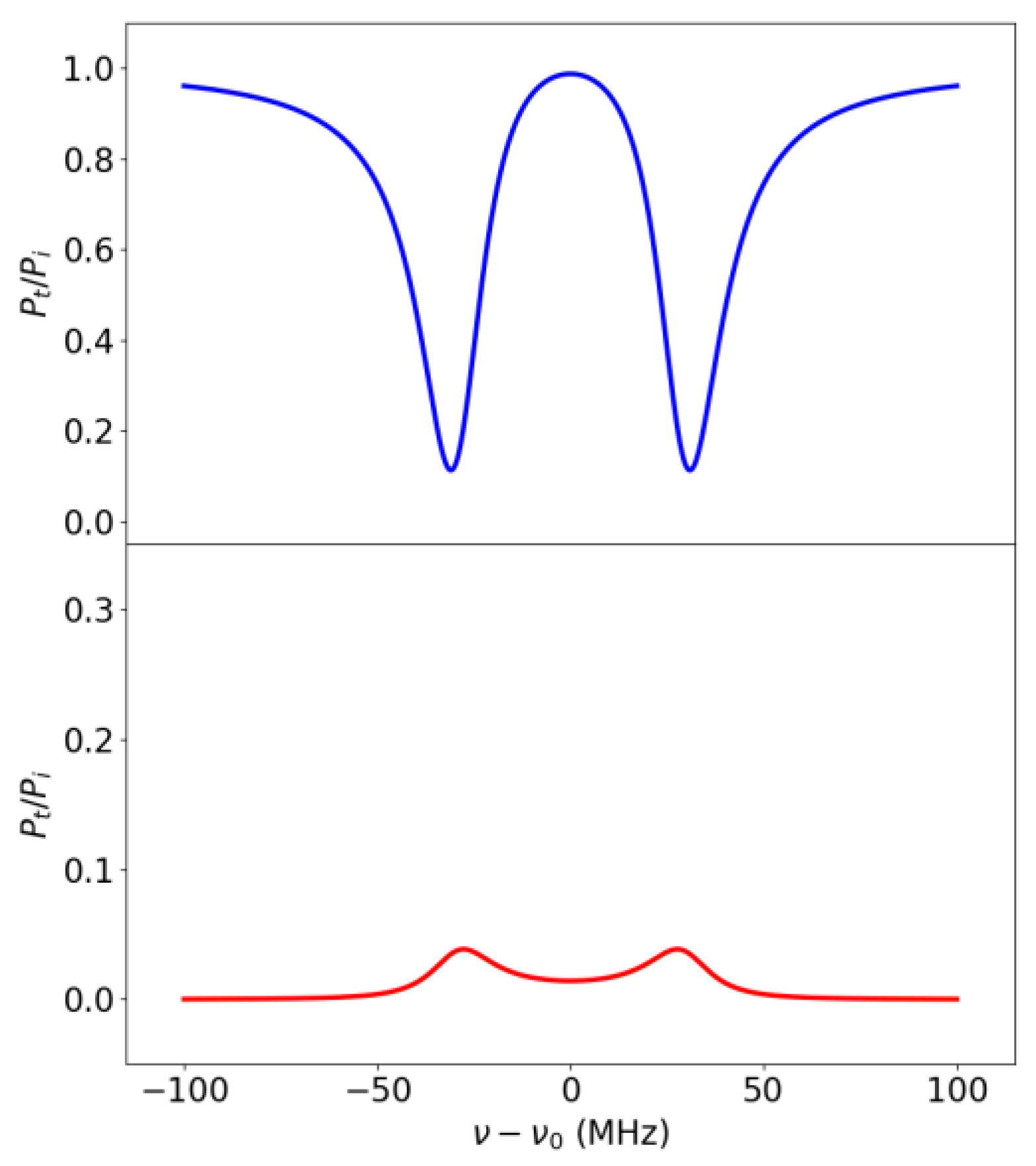
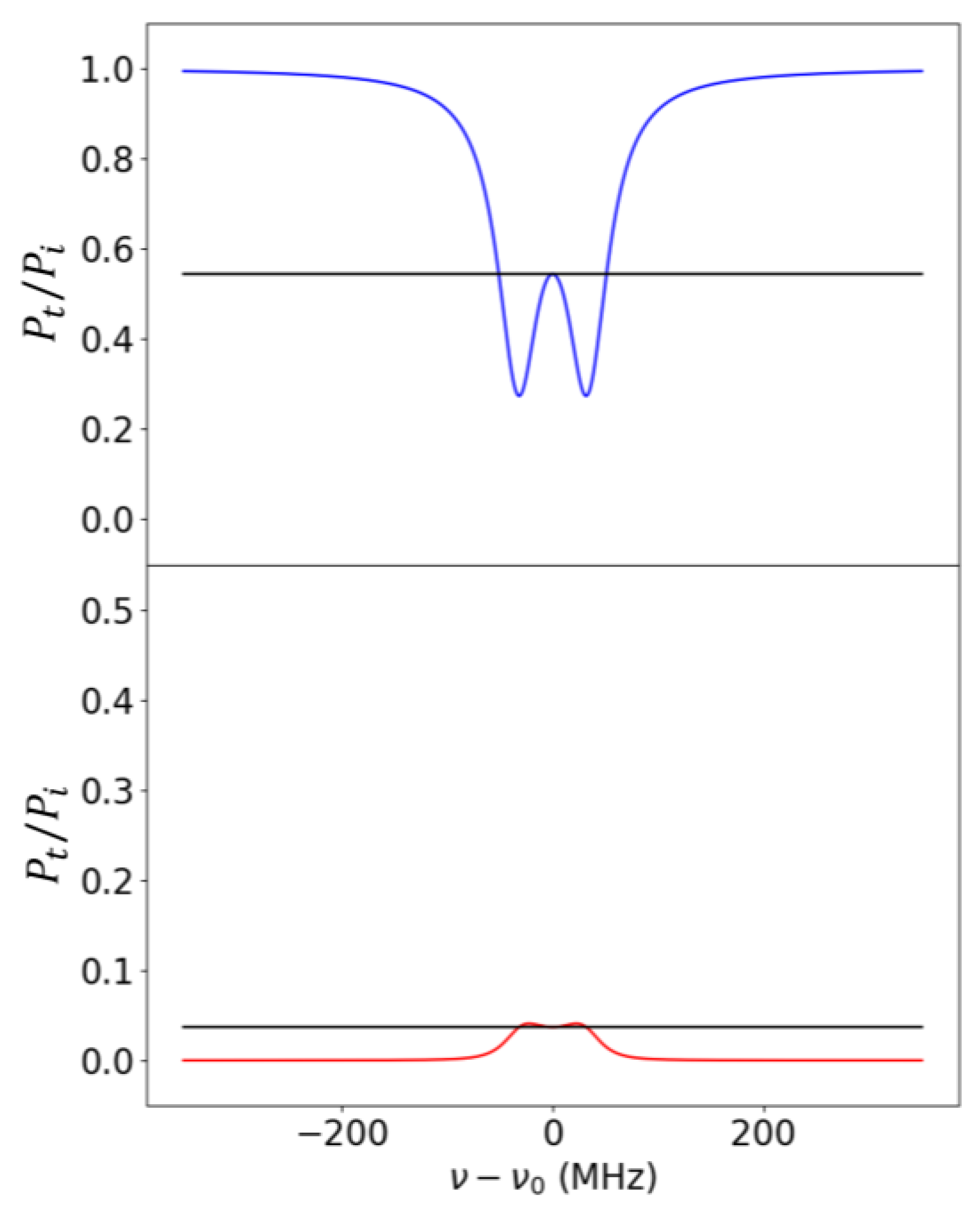
The resonant frequency of the driven polarization is the frequency reference, ν0 = ν1. The values of Tc and b are then varied; Tc is adjusted to fit the experimental mode 1 throughput spectrum and, in an extension to our previous analyses, b is varied to fit the experimental mode 2 output spectrum, thereby determining the CPC strength and asymmetry. To illustrate what this model predicts, Figure 1 shows a simulated case of ATS (CMIT becomes ATS when the coupling is strong enough that ), showing the throughput spectra of the two modes. The assumed parameter values are all experimentally realistic, and here we can neglect the small difference between n1 and n2. Frequency-split dips are observed in the mode 1 throughput and split peaks in the mode 2 output.
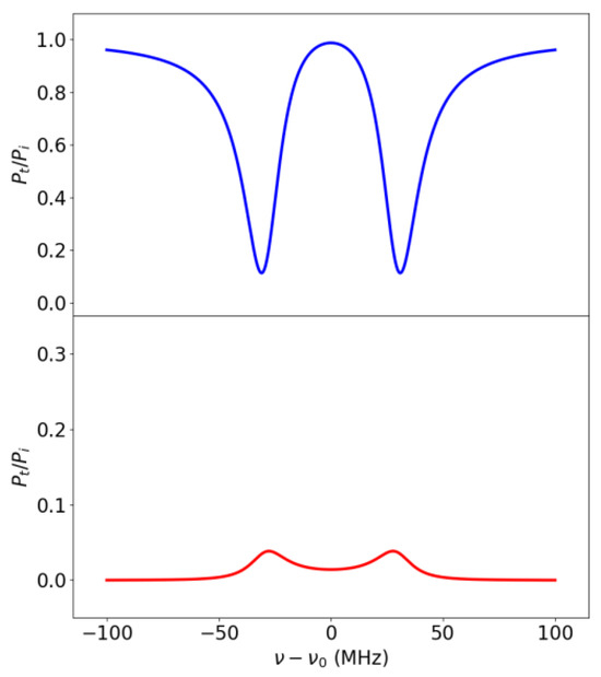
Figure 1.
ATS simulated in a microresonator of 90 µm radius. Upper: mode 1 throughput (blue); lower: mode 2 output (red). Parameter values: Q1 = 5 × 10⁶, Q2 = 2 × 10⁸; M1 = 0.9 (undercoupled), M2 = 0.1 (undercoupled); ∆ = 0 MHz. Assumed CPC strength and asymmetry parameter: Tc = 1.79 × 10⁻⁷ and b = 4.
The basic model presented here was developed further for this study to give analytical expressions for the CPC strength Tc and the asymmetry parameter b. These extensions are discussed in the Results section, below.
2.1.2. Detailed Theory
The detailed theory of CPC [20] uses the spatial field distributions of WGMs in a hollow bottle resonator (HBR) [24,25,26] to evaluate the cross-polarization coupling. A WGM has a radial structure that is described by Bessel functions of order m, having p radial intensity peaks, and an axial profile that is like a harmonic oscillator wave function consisting of a Gaussian multiplied by a Hermite polynomial of order q [24,25]. The WGM is thus characterized by the three mode numbers m (essentially the number of wavelengths per round trip), p (the number of radial intensity lobes), and q (the number of axial zeroes of intensity). Because the only one of these three mode numbers that can reliably be measured in an experiment is q, in the work reported here we did not try to determine any mode numbers experimentally. Therefore, in the theoretical calculations, representative sets of mode numbers are used that give values of Tc and b in the same range as the values found by fitting the simple model to the experimental throughput spectra. (The value of q can be found, in principle, by moving a second tapered fiber axially on the other side of the HBR and monitoring the number of minima in the outcoupled power while the individual mode parameters are being measured.)
Cross-polarization coupling in an HBR is possible if the resonator has some axial asymmetry, making the mean value of the axial component of the wavevector of each WGM nonzero, as illustrated in [20]. The magnitude of the wavevector is the propagation constant; for mode j, it is:
and is its mean axial component. In Equation (8), β0 is the propagation constant in a vacuum and a = L/2π is the HBR radius. The CPC amplitude t21 for coupling from mode 1 to mode 2 is calculated by taking into account the radial and axial spatial overlap of the two WGMs (represented by a factor I0, the result of an integral that is calculated numerically), the mean axial component of the source (mode 1) wavevector, and a phase-mismatch factor that depends on the difference in propagation constants, Δβ = |β1 − β2|. This gives:
where the last factor represents the phase mismatch between modes 1 and 2; t12 is found by interchanging 1 and 2 in Equation (9). In our original treatment [20], Tc = t21t12 was then calculated numerically.
This detailed theory was developed further for this study to give analytical expressions for the CPC strength Tc and the asymmetry parameter b. In addition, an analytical approximation for b with obvious physical significance was discovered. These extensions and a comparison of the analytical approximation for b with its value found from the full numerical calculation are discussed in the Results section, below.
2.2. Experimental Procedure
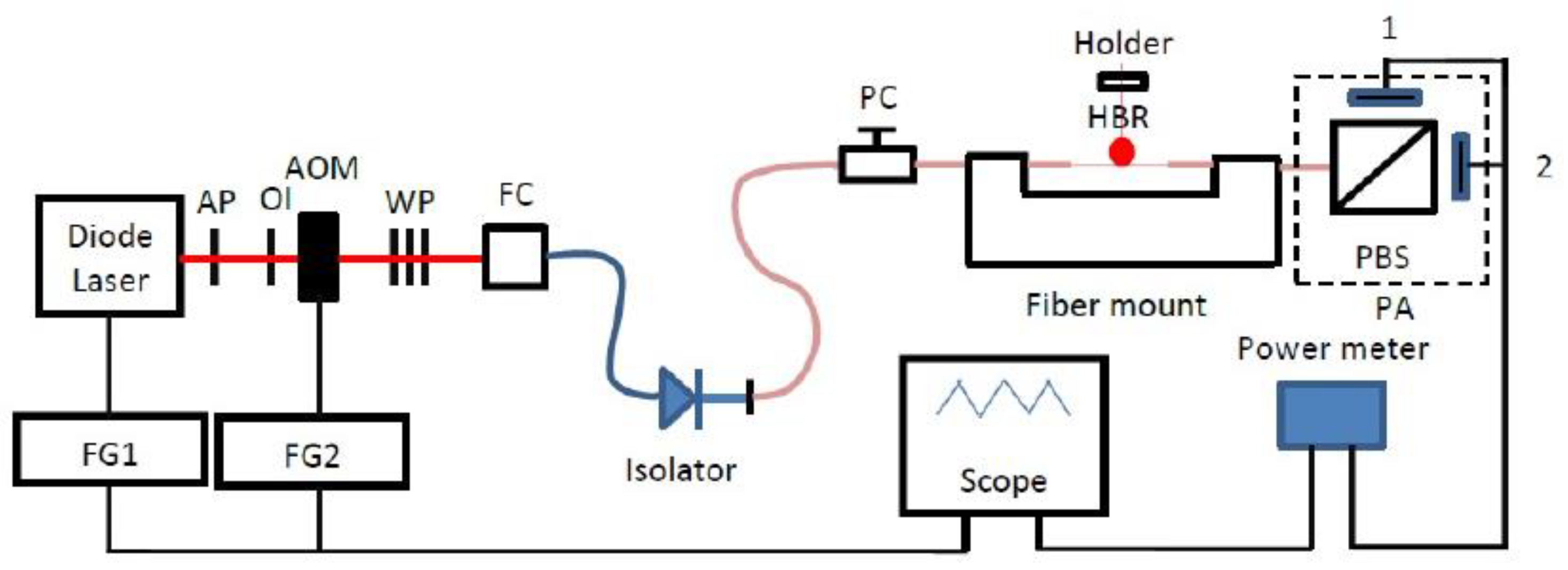
The experimental setup that we used is shown in Figure 2 [21]. The tunable diode laser emits at a wavelength of about 1550 nm, is scanned in frequency by a signal from the frequency generator FG1, and its free-space beam passes through an acousto-optic modulator, which was not used in this work. Wave plates (WP) and a compression-based polarization controller (PC) were used to control the input polarization. The coupling fiber was adiabatically bitapered and brought into contact with the HBR in its equatorial plane (cross section with maximum diameter) using a 3D translation stage that is not shown. The HBR was mounted on a piezo-controlled holder for strain tuning, as described in more detail below. The length of fiber after the HBR was kept short and straight to preserve the polarization. In all cases, the resonator was kept inside an acrylic box to minimize temperature fluctuations and other effects of air movement. The output signal is sent to a polarization analyzer (PA), which includes a polarizing beam splitter (PBS) plus two matched fast detectors (1 and 2); the entire PA system can be rotated about the fiber axis so that either detector can detect either polarization. For data analysis, the detector signals were separately input to the oscilloscope, without using the power meter shown in Figure 2.
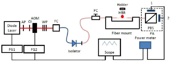
Figure 2.
Experimental setup [21]. Light from a tunable diode laser frequency-scanned by FG1 passes through an anamorphic prism (AP), an optical isolator (OI), an acousto-optic modulator (AOM, not used here), and wave plates (WP); a fiber coupler (FC) injects it into a fiber isolator and the polarization is further adjusted using the polarization controller (PC) before it enters the tapered section, where it is coupled into a WGM of the hollow bottle resonator (HBR). The output power undergoes polarization analysis (PA) and detection.
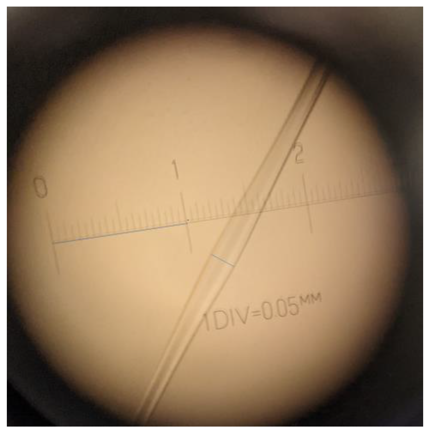
The hollow bottle resonator (HBR) was fabricated [26] by heating and pressurizing a 150 μm diameter silica capillary to create a bulge of about 195 μm in diameter, as shown in Figure 3. On either side of the bulge, the HBR was glued to a flexible mount that was actuated by a piezoelectric crystal that expands with applied voltage, stretching the HBR. The induced strain shifts the WGM resonant frequencies by different amounts for TE and TM, allowing orthogonally polarized modes to be brought into and out of coresonance [21]. The limited amount of strain tuning that is needed to do this does not change the depth or width of either mode’s throughput dip.

Figure 3.
Hollow bottle resonator with an equatorial (bulge) diameter of 195 μm.
In the experiments, the input light was linearly polarized to excite either TE or TM WGMs. This was achieved by rotating the PA by 45° or temporarily removing the PBS so that dips corresponding to the WGMs of both polarizations could be observed. Then, the input polarization was adjusted to remove half of those (one polarization), and the PA was rotated back so that only one detector received a signal. The detectors at the outputs of the polarizing beam splitter are monitored by an oscilloscope so that each polarization throughput is displayed on a separate channel. If we label the channels according to the convention used in the Introduction, channel 1 corresponds to the input polarization and channel 2 corresponds to the orthogonal polarization. If the input polarization is TE, channel 1 shows the detector 1 signal and channel 2 that of detector 2 (see Figure 2). If the input polarization is TM, channel 1 is the detector 2 signal and channel 2 shows that of detector 1. The HBR is stretched by the piezo controller, tuning the WGMs; whenever a TE mode is in resonance with a TM mode, a characteristic spectral shape of induced transparency or frequency splitting can be observed in the trace on the input polarization channel (1) on the oscilloscope. Simultaneously, channel 2 shows a trace of the spectral shape of the output of the orthogonal polarization.
After recording the observed spectra from the two polarization channels, the WGMs were detuned from coresonance again to characterize the two individual WGMs; the input polarization was rotated by 90° to take measurements for orthogonal mode 2. To characterize a WGM, the linewidth and depth of the resonant throughput dip were measured, and the coupling regime was determined by lightly touching the resonator with the tip of an additional fiber to add loss to the system and observe whether the dip became deeper or shallower [21]. These measurements then determined the coupling and intrinsic losses of the WGM, along with its quality factor Q, as explained in the theory section above.
Once all parameters were measured, they were used in the numerical simulation, where the CPC amplitudes t21 and t12 were at this point the only unknown parameters. The recorded traces from the oscilloscope were plotted along with the simulation, and the coupling strength Tc and coupling ratio b were left as free adjusting parameters to fit the simulated throughput to the experimental data. (It may happen that perfect coresonance is not achieved when recording the traces; in that case, the detuning of mode 2 from mode 1 enters as a semi-free parameter.) To perform this fitting, we developed an algorithm that allowed us to crop, scale, and center the traces obtained from the oscilloscope to the same scaling used in the computational model, along with a graphical user interface that enabled the free parameters to be easily changed for an optimal fit.
This procedure was repeated for many different cases, all of which turned out to be ATS due to the relatively strong CPC and the ratio of the WGM quality factors not being large in comparison to unity. We attempted to increase this ratio by adding additional loss to mode 1, decreasing its Q, but were not able to observe CMIT. This extra loss was to be provided by the interaction of WGM 1 with water or methanol inside the HBR, allowing the WGM to experience additional loss due to absorption in its internal fraction. Not having cases that were CMIT was not a problem, because ATS spectra are even more suitable for the determination of the value of the asymmetry parameter b.
3. Results
In this section, we present both theoretical and experimental results. The theoretical results consist of our new extensions of the basic model, which describes CPC from the perspective of mode amplitudes and on which our numerical simulations are based [21], and our new extensions of the detailed theory that describes CPC from the perspective of the spatial structure of the WGMs that couple to each other [20]. The experimental results include throughput spectra that allow us to determine the CPC strength and asymmetry parameter, as well as comparison to the simulated behavior and interpretations of their similarities and differences.
3.1. New Theory Developments
3.1.1. Basic Model and Simulation
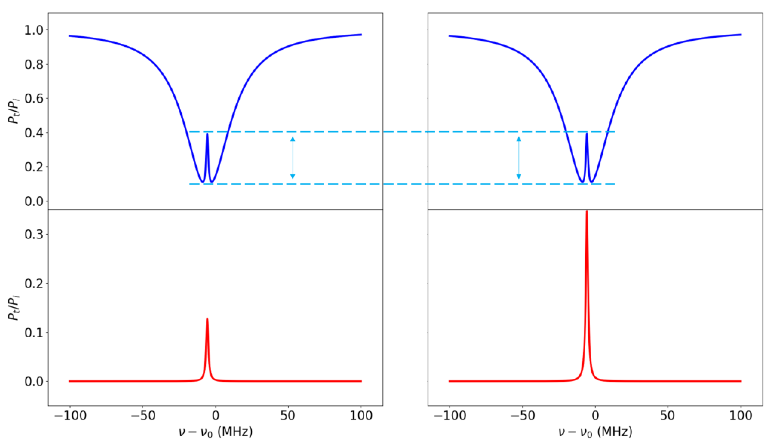
In addition to the new fitting of the mode 2 output to determine the experimental value of b, the basic model was developed further for this study to give analytical expressions for the CPC strength Tc and the asymmetry parameter b. The significance of Tc and b can be seen more directly in Figure 4, where the numerical model described in Section 2.1.1, above, was used to simulate two cases with experimentally realistic parameter values. In these cases, Tc is small enough that mode 1 shows a CMIT feature and mode 2 shows a single peak. In the left and right panels, the value of Tc is the same and the mode 1 throughput spectra are identical. Left and right have different values of b, and the height of the mode 2 peak is seen to be proportional to b.
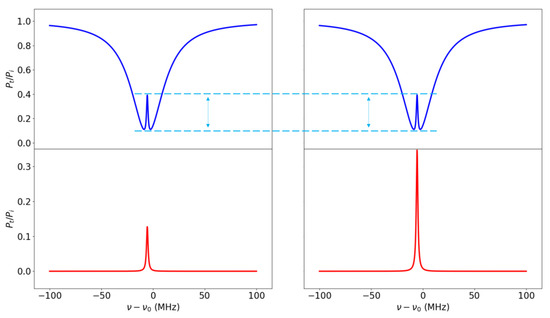
Figure 4.
CMIT simulated in an HBR of 98 µm radius. Upper: mode 1 throughput (blue); lower: mode 2 output (red). Parameter values: Q1 = 5 × 10⁶, Q2 = 2 × 10⁸; M1 = 0.9 (undercoupled), M2 = 0.5 (undercoupled); ∆ = 0 MHz. Assumed CPC strength: Tc = 2.65 × 10⁻⁸. Assumed asymmetry parameter: left, b = 2.56; right, b = 6.97.
The relative output powers at the central peaks, or more generally, the local maximum or minimum on resonance, can be found analytically from our model Equations (1)–(3). If ∆ = 0 and the input is tuned to the two-mode coresonance, ν = ν0, Equation (3) shows that γj = κj. Making that substitution in Equation (2) and solving in a steady state, using the very good approximation that T1 + α1L << 1 and not assuming that n1 = n2, we find the resonant values of the relative powers of Equation (7):
and, with another very good approximation that r1 = 1:
Equations (10) and (11) represent a further extension of the basic model and illustrate analytically what was seen in the numerical results of Figure 4, that the mode 1 throughput depends on Tc but not b and that the mode 2 output is proportional to b. The validity of the approximations made in the derivation of Equations (10) and (11) is confirmed by the fact that in every one of fifteen cases using widely varying parameters, these analytical expressions for resonant relative output powers agree with the full numerical solution to better than 1%. An example is shown in Figure 5, where the horizontal black lines are at the values of R1(0) and R2(0) calculated from Equations (10) and (11) and are tangent to the local maximum and local minimum of the numerical spectra, respectively.
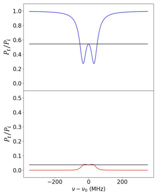
Figure 5.
CMIT simulated in an HBR of 90 µm radius. Upper: mode 1 throughput (blue); lower: mode 2 output (red). Black horizontal lines: values of R1(0) and R2(0) calculated from Equations (10) and (11). Parameter values: Q1 = 3.5 × 10⁶, Q2 = 4.8 × 10⁶; M1 = 0.95 (undercoupled), M2 = 0.38 (undercoupled); ∆ = 0 MHz. Assumed CPC strength: Tc = 3.11 × 10⁻⁷. Assumed asymmetry parameter: b = 1.00.
The agreement illustrated in Figure 5 then allows us to further extend our model to an alternative method for finding Tc and b, provided Δ is not too large; recall that Equations (10) and (11) were derived assuming ∆ = 0. Experimental values of R1(0) and R2(0) can be measured from the oscilloscope traces and inserted into the following equations:
derived from Equation (11); and derived from Equation (10):
How well this works will be discussed below in the subsection on experimental results.
3.1.2. Detailed Theory
The detailed theory described in Section 2.1.2, above, was also analytically extended for this study to give expressions for the CPC strength Tc and the asymmetry parameter b. In addition, an analytical approximation for b was discovered. These extensions, and a comparison of the approximate analytical and full numerical methods for finding b, are discussed here. Because Δβ << βj, the phase-mismatch factor in Equation (9) reduces to 2π/m1, so the CPC strength is given by:
which still depends on the numerically calculated overlap integral I0. However, in the asymmetry factor, the overlap integral is cancelled out since it is common to the two amplitudes:
At this point, we assume that, to lowest order, the mean axial component of the wavevector is simply proportional to the axial extent of the WGM. Recalling that the axial profile is a harmonic oscillator wave function, our assumption is , and with the use of Equation (8), we find an analytical approximation for the asymmetry parameter in which the dependence on the ratio of effective indices nj is essentially canceled by the dependence on the ratio of azimuthal mode orders mj:
Several (35) different cases using a large range of individual mode numbers (m1, m2, p1, p2, q1, q2) were calculated numerically using the full detailed theory of [20], producing CPC strengths ranging from 10–4 to 10–13 and asymmetry parameters ranging from 0.2 to 4.4. For each case, b was also calculated from the approximation of Equation (16), and the two values of asymmetry parameter are compared in Figure 6.
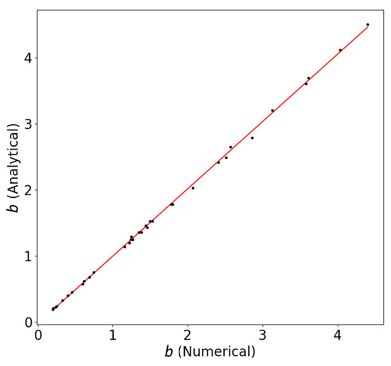
Figure 6.
Comparing the analytical approximation of Equation (16) for the asymmetry parameter and its numerically calculated value from the full detailed theory. The red line is a linear fit to the data points given by the equation .
These analytical extensions to the detailed theory of [20] now show that the major contributor to asymmetry in CPC is the different axial extent of the two coupled WGMs. The contribution of the effective index of refraction, which comes into the approximation for the mean axial component of the wavevector, ends up being removed because of the difference in the mode numbers mj. The quality of the analytical approximation for b is evident from Figure 6, where the slope of a linear fit to the data is very nearly equal to 1. Closer inspection shows that the approximation for b values less than 1 tends to produce slightly lower values, and the approximation for b values greater than 1 tends to produce slightly higher values. This results in the slope of the linear fit being slightly greater than 1 (1.02). This could be investigated further in future studies. The experimental parts of those studies could also include measurements to find the values of q1 and q2 and enable a direct experimental test of Equation (16).
3.2. Experimental Results
After the experimental procedure described in Section 2 was perfected on several preliminary HBR systems, 19 careful experiments were performed using frequency-scanned input light of 1550 nm wavelength. In these experimental cases, the input polarization was TE or TM; the HBR radius varied from 89 μm to 172 μm; and the quality factors, resonant dip depths, and coupling regimes of the individual WGMs took on many different values. The HBRs were filled with air, methanol, or water; as noted, the filling only affects the values of one or both quality factors. The experimentally measured parameters of the individual WGMs were put into the numerical model, which was overlaid on the experimental traces as described in Section 2.2; then, Tc was adjusted to fit the mode 1 throughput while b was adjusted to fit the mode 2 output. Several examples are shown in the figures that follow, where the analytical approximate values of Tc and b found from Equations (12) and (13) are also listed in the captions for comparison with the fitted values.
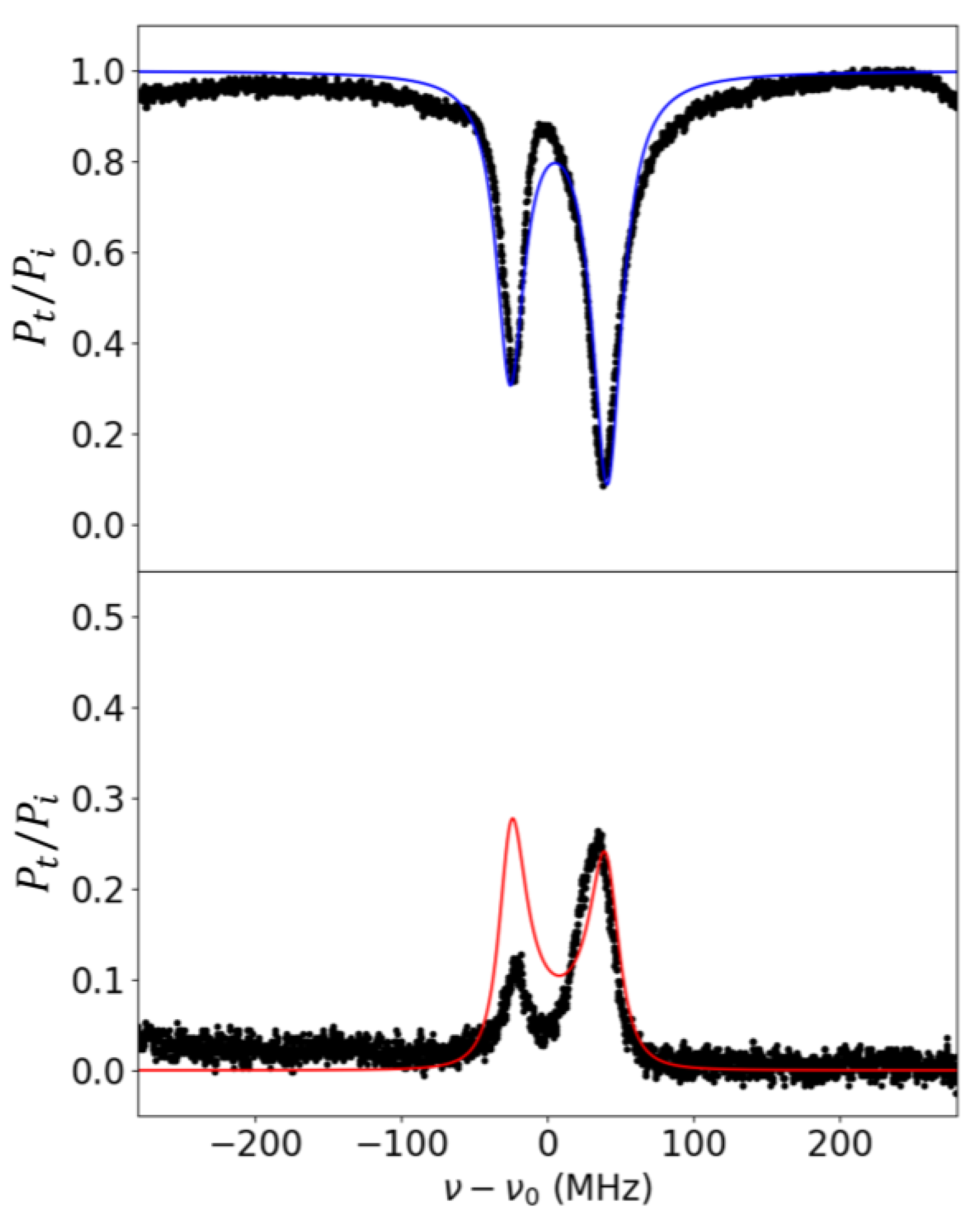
Figure 7 shows one example. Like our simulations in Figure 1, Figure 4, and Figure 5, the upper part of the figure is the mode 1 throughput, and the lower part is the mode 2 output, but now the experimental traces are in black and the fitted numerical simulation is represented by the blue and red curves.
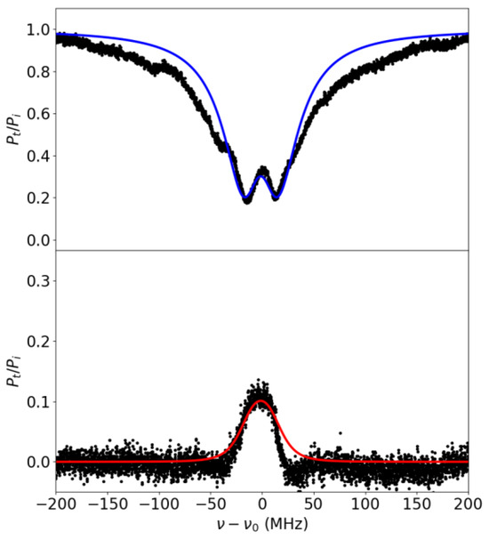
Figure 7.
ATS observed in an air-filled HBR of 172 µm radius with TE input. Upper: mode 1 throughput; lower: mode 2 output. Black: experimental spectra; blue and red: numerical fitting. Parameter values: Q1 = 3.13 × 10⁶, Q2 = 7.29 × 10⁶; M1 = 0.923 (undercoupled), M2 = 0.296 (undercoupled); ∆ = 0 MHz. Coupling strength and asymmetry parameter found by fitting: Tc = 3.30 × 10⁻⁷, b = 3.7. Coupling strength and asymmetry parameter found from the approximations of Equations (12) and (13): Tc = 3.20 × 10⁻⁷, b = 3.9.
In our results, deviations of the experimental spectra from the fitted numerical model are almost always due to the presence or near-overlap of additional modes that do not take part in cross-polarization coupling. For mode 1, the next two figures show obvious examples; for mode 2, an extra mode that shows no CPC will not be seen, but if it couples to the WGM of the polarization 2 that takes part in CPC, significant deviations can occur, as will be discussed later. The asymmetry of the mode 2 experimental trace in Figure 7 may be a result of a second mode of the same polarization that couples weakly to it, without undergoing CPC itself. The uncertainty in the fitted value of Tc is about 20%, which is reasonable considering that Tc can range over several orders of magnitude. The uncertainty in the fitted b is probably about 10% when no other modes of polarization 2 are involved. Uncertainties in the approximate values of Tc and b are roughly the same as for the fitted values but more difficult to estimate, as the values found can be affected by the same factors as the fitting values and also depend on asymmetry of the spectra caused by nonzero 2–1 detuning Δ, since Equations (12) and (13) assume Δ = 0. In Figure 7, Δ = 0 and the two methods agree to well within the fitting uncertainties.
Figure 8 shows another example. Unlike the case of Figure 7, Δ is now a significant fraction of the width of the entire ATS feature in the mode 1 throughput, so we expect the approximate values of Tc and b to be less reliable. As expected, the two methods for finding Tc and b agree less well. In particular, the disagreement in Tc may be a result of the poorer fit of the central peak in the ATS feature (R1(0)). Note the extra dip on the left side of the experimental mode 1 trace, indicating a nearby WGM of polarization 1 that is far enough away from coresonance that it does not affect the fitting. The lack of a corresponding peak in the mode 2 trace shows that there is no CPC at this frequency due to the lack of a coresonant mode of polarization 2.
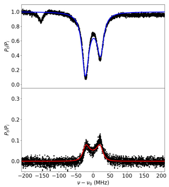
Figure 8.
ATS observed in a water-filled HBR of 90 µm radius with TM input. Upper: mode 1 throughput; lower: mode 2 output. Black: experimental spectra; blue and red: numerical fitting. Parameter values: Q1 = 8.05 × 10⁶, Q2 = 8.05 × 10⁶; M1 = 1.0 (critically coupled), M2 = 0.566 (undercoupled); ∆ = 13.1 MHz. Coupling strength and asymmetry parameter found by fitting: Tc = 1.39 × 10⁻⁷, b = 1.0. Coupling strength and asymmetry parameter found from the approximations of Equations (12) and (13): Tc = 2.14 × 10⁻⁷, b = 1.2.
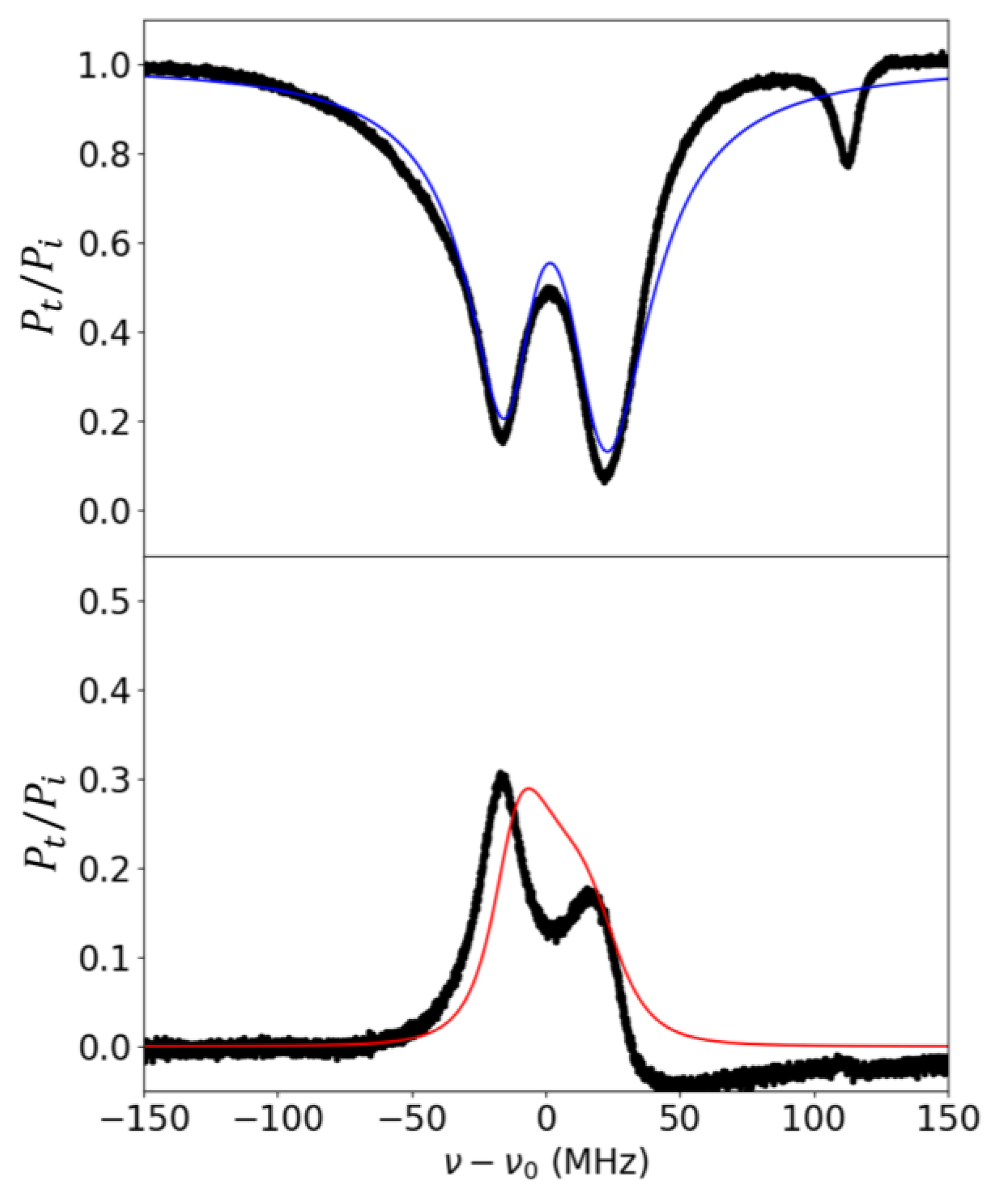
Other cases are shown in Figure 9 and Figure 10, the first with a smaller relative value of Δ, and the second with a larger Δ. As in Figure 7 and Figure 8, the model fitting in Figure 9 is relatively good in that both experimental traces are reproduced qualitatively and quantitatively by the model. Again, we see the effect of Δ on the agreement of the two methods for finding Tc and b, with Figure 9 showing better agreement than Figure 10. Figure 10 also shows the effect on the approximate method of having a fitting disagreement in the central part of the feature, as noted in Figure 8, but in this case in both polarizations (R2(0) as well as R1(0)). In Figure 10, the asymmetry in the mode 2 experimental trace is opposite that of the model, even though the model fits the mode 1 trace well. This is most likely to be due again to the interaction of another mode of polarization 2.
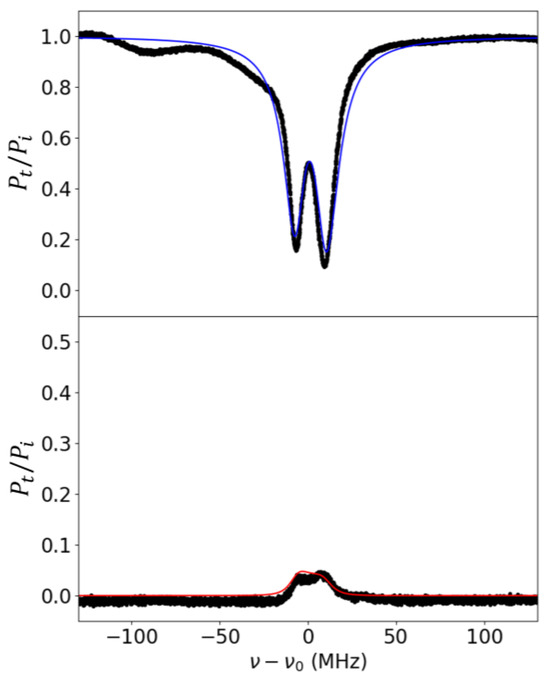
Figure 9.
ATS observed in an air-filled HBR of 98 µm radius with TE input. Upper: mode 1 throughput; lower: mode 2 output. Black: experimental spectra; blue and red: numerical fitting. Parameter values: Q1 = 8.8 × 10⁶, Q2 = 2.26 × 10⁷; M1 = 0.95 (undercoupled), M2 = 0.13 (undercoupled); ∆ = −2.3 MHz. Coupling strength and asymmetry parameter found by fitting: Tc = 2.26 × 10⁻⁸, b = 3.7. Coupling strength and asymmetry parameter found from the approximations of Equations (12) and (13): Tc = 2.16 × 10⁻⁸, b = 2.7.
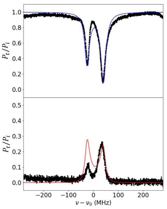
Figure 10.
ATS observed in an air-filled HBR of 89 µm radius with TM input. Upper: mode 1 throughput; lower: mode 2 output. Black: experimental spectra; blue and red: numerical fitting. Parameter values: Q1 = 7.06 × 10⁶, Q2 = 9.39 × 10⁶; M1 = 1.0 (critically coupled), M2 = 0.30 (overcoupled); ∆ = −21 MHz. Coupling strength and asymmetry parameter found by fitting: Tc = 2.97 × 10⁻⁷, b = 0.62. Coupling strength and asymmetry parameter found from the approximations of Equations (12) and (13): Tc = 5.87 × 10⁻⁷, b = 0.48.
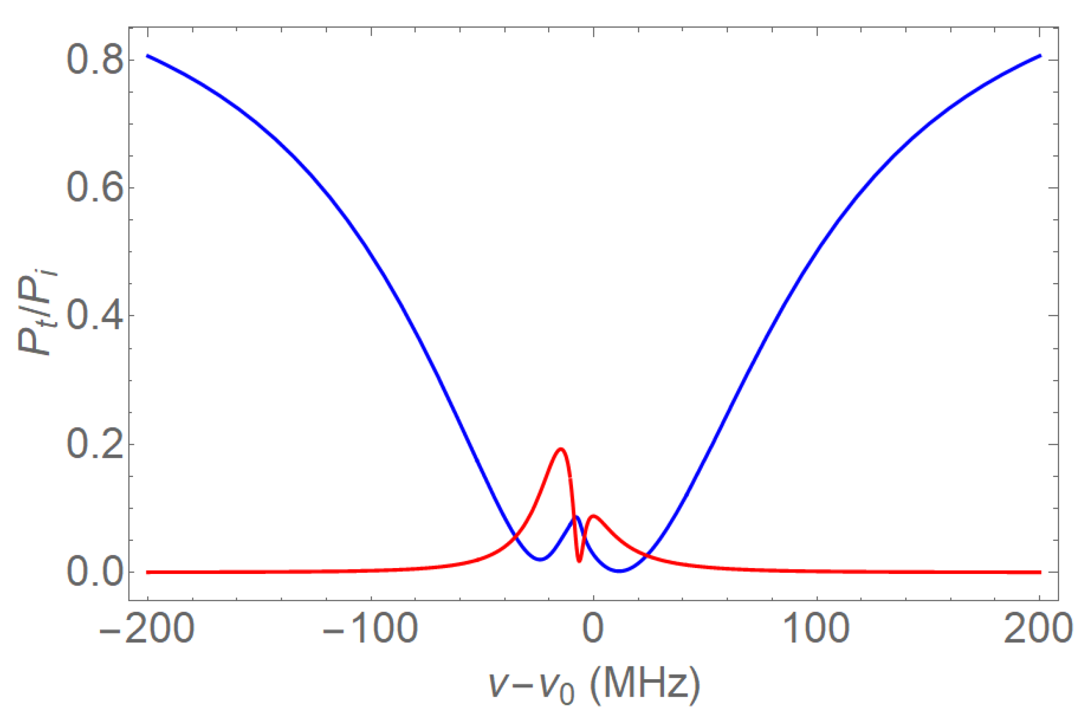
Even stronger discrepancies in polarization 2 between experiment and model are seen in Figure 11 and Figure 12, where the model reproduces the mode 1 throughput well. In these two cases, the experimental trace shows a dip that is not predicted by the two-mode model. To test our hypothesis that these effects are due to the interaction of a second mode of polarization 2, we revised our model. In the revised model, there are still two modes of orthogonal polarizations that interact via CPC, but there is a second mode of polarization 2 that interacts with the other mode 2 by fiber-mediated coupling—light in one WGM couples out into the fiber and then immediately back into the other mode of the same polarization. One example of the output of this revised model is shown in Figure 13, supporting our conjecture. Other cases using the revised model also typically show relatively sharp dips in the mode 2 output, like that in Figure 13 and those in the mode 2 experimental output traces in Figure 11 and Figure 12.

Figure 11.
ATS observed in an air-filled HBR of 172 µm radius with TE input. Upper: mode 1 throughput; lower: mode 2 output. Black: experimental spectra; blue and red: numerical fitting. Parameter values: Q1 = 3.65 × 10⁶, Q2 = 1.37 × 10⁷; M1 = 0.933 (undercoupled), M2 = 0.938 (overcoupled); ∆ = −6.0 MHz. Coupling strength and asymmetry parameter found by fitting: Tc = 3.39 × 10⁻⁷, b = 2.3. Coupling strength and asymmetry parameter found from the approximations of Equations (12) and (13): Tc = 3.12 × 10⁻⁷, b = 1.4.
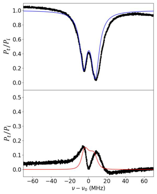
Figure 12.
ATS observed in an air-filled HBR of 172 µm radius with TE input. Upper: mode 1 throughput; lower: mode 2 output. Black: experimental spectra; blue and red: numerical fitting. Parameter values: Q1 = 9.99 × 10⁶, Q2 = 1.50 × 10⁷; M1 = 1.0 (critically coupled), M2 = 1.0 (critically coupled); ∆ = −2.77 MHz. Coupling strength and asymmetry parameter found by fitting: Tc = 4.09 × 10⁻⁸, b = 0.62. Coupling strength and asymmetry parameter found from the approximations of Equations (12) and (13): Tc = 4.00 × 10⁻⁸, b = 0.66.
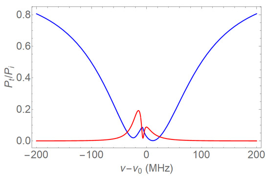
Figure 13.
Simulation involving three modes nearly coresonant with each other, one of polarization 1 and two of polarization 2. Blue: polarization 1 throughput, showing ATS due to the interaction of the two orthogonal modes coupled by CPC. Red: polarization 2 output, showing additional sharp structure due to the interaction of the two modes of polarization 2.
The other experimental cases that were assessed revealed results like those presented here. The quality factors of the individual WGMs ranged from 1.0 × 10⁶ to 3.4 × 10⁷, the CPC strengths (Tc) found ranged from 1.5 × 10⁻⁸ to 3.4 × 10⁻⁷, and the asymmetry parameters (b) found ranged from 0.18 to 4.1. These ranges are consistent with those of Tc and b found from the detailed theory for reasonable sets of mode numbers. The agreement between the fitting method and the approximate method for determining Tc and b was reasonable as long as the 2–1 detuning Δ was not too large a fraction of the feature width and no effects of third-mode coupling were observed.
4. Discussion
We have previously shown theoretically that cross-polarization coupling is asymmetrical, with the amplitude per round trip for coupling from mode 1 to mode 2 differing, in general, from the mode 2 to mode 1 coupling amplitude [20]. Here, we have confirmed this asymmetry experimentally by detecting the output spectra for both polarizations and determining the asymmetry parameter, which is the ratio of the two amplitudes. Two methods were used to measure the CPC strength, which is the product of the two amplitudes, along with the asymmetry parameter. One method relies on fitting the experimental output spectra to a simple model, as in [21], but now extended to the output of the orthogonal polarization as well as that of the input polarization. The other method is based on an analytical extension of the simple model in Section 2.1.1, as described in Section 3.1.1. The fitting method works well, with uncertainties of about 20% in the CPC strength and 10% in the asymmetry parameter, and the other method works equally well if the two modes are close to coresonance, and no other modes of orthogonal polarization (2) are involved. The main experimental difficulty comes from the presence of these additional polarization-2 modes of the microresonator that do not interact via CPC but affect the agreement with the model by their interaction with a mode of the same polarization. The model was extended to account for this other interaction involving a third mode, and the polarization-2 output spectra that it produced were in qualitative agreement with the experimental observations. Our new approximate analysis of the detailed theory of [20] shows that the asymmetry parameter is nearly exactly equal to the ratio of the axial extent of mode 1 to the axial extent of mode 2, and the approximation gives the same value of b as determined from numerical solution of the detailed theory.
In both the experiment and in the detailed-theory calculation, the CPC strength Tc most often took values of the order of 10–8 or 10–7; very few calculated values were significantly larger or smaller than this range. In both experiment and theory, the asymmetry parameter b was typically smaller than 0.8 or larger than 1.3; few cases showed very little asymmetry, with b~1. The few calculated cases that did show low asymmetry seem to have been correlated with particularly large values of Tc, and extreme asymmetry seemed to be correlated with especially small values of Tc. These trends do not seem to have an obvious explanation and represent an interesting topic for further analysis.
Further experimental work should include measurements of the axial mode numbers qj of the individual WGMs to test the theoretical approximation of Equation (16). This may be difficult given the overall stability of the system but should be feasible and would provide another strong test of the theory. Investigation of asymmetric mode coupling could be extended to coupled-resonator-induced transparency (CRIT) [1,2,3], where input light excites a WGM of one microresonator that then couples to a WGM of the same polarization in a second nearby resonator. In the case of CRIT, a second fiber would be needed to sample the output coupled from the WGM of the second microresonator, which would be analogous to the orthogonal polarization output in this work.
Finally, note that the intracavity mode amplitudes of Equation (2) can be written in two-vector form, where then the time-evolution matrix on the right-hand side of the equation can be interpreted as a non-Hermitian Hamiltonian. Further study of systems that show asymmetric mode coupling might be used to investigate the exciting world of non-Hermitian physics [27]. One possibility would involve increasing the value of Tc in the model to make it greater than the other losses, Tj + αjL. Within this limit, nonreciprocity in the propagation of light in the system might be observable. This limit could be achieved experimentally by adding some gain to offset the other microresonator losses.
Author Contributions
Conceptualization, A.T.R. and K.S.; methodology, K.S.; software, K.S. and A.T.R.; validation, K.S. and A.T.R.; formal analysis, K.S. and A.T.R.; investigation, K.S.; resources, A.T.R.; data curation, A.T.R.; writing—original draft preparation, K.S. and A.T.R.; writing—review and editing, K.S. and A.T.R.; visualization, K.S.; supervision, A.T.R.; project administration, A.T.R.; funding acquisition, A.T.R. All authors have read and agreed to the published version of the manuscript.
Funding
This research received partial support from the Oklahoma State University College of Arts and Sciences Research Program. The APC was waived.
Institutional Review Board Statement
Not applicable.
Informed Consent Statement
Not applicable.
Data Availability Statement
Data are available from the corresponding author upon request.
Acknowledgments
We would like to thank Sreekul Raj Rajagopal for assistance with the initial experiments and Mohmad Junaid Ul Haq for assistance with some calculations.
Conflicts of Interest
The authors declare no conflicts of interest. The funders had no role in the design of the study; in the collection, analyses, or interpretation of the data; in the writing of the manuscript; or in the decision to publish the results.
References
- Naweed, A.; Farca, G.; Shopova, S.I.; Rosenberger, A.T. Induced transparency and absorption in coupled whispering-gallery microresonators. Phys. Rev. A 2005, 71, 043804. [Google Scholar] [CrossRef]
- Totsuka, K.; Kobayashi, N.; Tomita, M. Slow light in coupled-resonator induced transparency. Phys. Rev. Lett. 2007, 98, 213904. [Google Scholar] [CrossRef] [PubMed]
- Zhou, X.; Zhang, L.; Pang, W.; Zhang, H.; Yang, Q.; Zhang, D. Phase characteristics of an electromagnetically induced transparency analogue in coupled resonant systems. New J. Phys. 2013, 15, 103033. [Google Scholar] [CrossRef]
- Ren, L.; Wen, H.; Shi, L.; Zhang, X. Electromagnetically induced transparency with a single optomechanical microring resonator. Opt. Lett. 2022, 47, 1363–1366. [Google Scholar] [CrossRef] [PubMed]
- Yi, C.-J.; Shen, M.-C.; Qin, Q.; Zhang, Y.-F.; Lin, X.-M.; Ye, M.-Y. Transition from electromagnetically-induced transparency to absorption in a single microresonator. Opt. Express 2023, 31, 7167–7174. [Google Scholar] [CrossRef] [PubMed]
- Qin, H.; Ding, M.; Yin, Y. Induced Transparency with Optical Cavities. Adv. Photonics Res. 2020, 1, 2000009. [Google Scholar] [CrossRef]
- Zhu, J.; Ozdemir, S.K.; Xiao, Y.-F.; Li, L.; He, L.; Chen, D.-R.; Yang, L. On-chip single nanoparticle detection and sizing by mode splitting in an ultrahigh-Q microresonator. Nat. Photonics 2010, 4, 46–49. [Google Scholar] [CrossRef]
- Fu, Y.; Qing, Y.M.; Li, Z.; Zayats, A.V.; Lei, D. Tale of Two Resonances: Waveguide-Plasmon Coupling and High Q-Factor Engineering on the Nanoscale. ACS Photonics 2023, 10, 2–12. [Google Scholar] [CrossRef]
- Foreman, M.R.; Swaim, J.D.; Vollmer, F. Whispering gallery mode sensors. Adv. Opt. Photon. 2015, 7, 168–240. [Google Scholar] [CrossRef]
- Yoshiki, W.; Honda, Y.; Tetsumoto, T.; Furusawa, K.; Sekine, N.; Tanabe, T. All-optical tunable buffering with coupled ultra-high Q whispering gallery mode microcavities. Sci. Rep. 2017, 7, 10688. [Google Scholar] [CrossRef]
- Smith, D.D.; Chang, H.; Myneni, K.; Rosenberger, A.T. Fast-light enhancement of an optical cavity by polarization mode coupling. Phys. Rev. A 2014, 89, 053804. [Google Scholar] [CrossRef]
- Guan, G.; Vollmer, F. Polarized transmission spectra of the fiber-microsphere system. Appl. Phys. Lett. 2005, 86, 121115. [Google Scholar] [CrossRef]
- Konishi, H.; Fujiwara, H.; Takeuchi, S.; Sasaki, K. Polarization-discriminated spectra of a fiber-microsphere system. Appl. Phys. Lett. 2006, 89, 121107. [Google Scholar] [CrossRef]
- Bianucci, P.; Fietz, C.R.; Robertson, J.W.; Shvets, G.; Shih, C.-K. Polarization conversion in a silica microsphere. Opt. Express 2007, 15, 7000–7005. [Google Scholar] [CrossRef] [PubMed]
- Ramelow, S.; Farsi, A.; Clemmen, S.; Levy, J.S.; Johnson, A.R.; Okawachi, Y.; Lamont, M.R.E.; Lipson, M.; Gaeta, A.L. Strong polarization mode coupling in microresonators. Opt. Lett. 2014, 39, 5134–5137. [Google Scholar] [CrossRef]
- Liu, Y.C.; Li, B.-B.; Xiao, Y.-F. Electromagnetically induced transparency in optical microcavities. Nanophotonics 2017, 6, 789–811. [Google Scholar] [CrossRef]
- Nasir, M.N.M.; Gorajoobi, S.B.; Murugan, G.S.; Zervas, M.N. Polarization effects in optical microresonators. J. Opt. Soc. Am. B 2019, 36, 705–716. [Google Scholar] [CrossRef]
- Kreismann, J.; Hentschel, M. Spin-orbit interaction of light in three-dimensional microcavities. Phys. Rev. A 2020, 102, 043524. [Google Scholar] [CrossRef]
- Wang, C.; Jiang, X.; Sweeney, W.R.; Hsu, C.W.; Liu, Y.; Zhao, G.; Peng, B.; Zhang, M.; Jiang, L.; Stone, A.D.; et al. Induced transparency by interference or polarization. Proc. Natl. Acad. Sci. USA 2021, 118, e2012982118. [Google Scholar] [CrossRef]
- Rosenberger, A.T.; Dale, E.B.; Bui, K.V.; Gonzales, E.K.; Ganta, D.; Ke, L.; Rajagopal, S.R. Cross-polarization coupling of whispering-gallery modes due to the spin-orbit interaction of light. Opt. Lett. 2019, 44, 4163–4166. [Google Scholar] [CrossRef]
- Bui, K.V.; Rosenberger, A.T. Coupled-mode-induced transparency and attenuation resulting from cross-polarization coupling. Phys. Rev. A 2020, 101, 033836. [Google Scholar] [CrossRef]
- Humphrey, M.J.; Dale, E.; Rosenberger, A.T.; Bandy, D.K. Calculation of optimal fiber radius and whispering-gallery mode spectra for a fiber-coupled microsphere. Opt. Commun. 2007, 271, 124–131. [Google Scholar] [CrossRef]
- Gorajoobi, S.B.; Murugan, G.S.; Zervas, M.N. Efficient excitation and phase matching of fiber-coupled degenerate whispering gallery modes. J. Opt. Soc. Am. B 2019, 36, 2452–2460. [Google Scholar] [CrossRef]
- Sumetsky, M. Whispering-gallery-bottle microcavities: The three-dimensional etalon. Opt. Lett. 2004, 29, 8–10. [Google Scholar] [CrossRef] [PubMed]
- Murugan, G.S.; Petrovich, M.N.; Jung, Y.; Wilkinson, J.S.; Zervas, M.N. Hollow-bottle optical microresonators. Opt. Express 2011, 19, 20773–20784. [Google Scholar] [CrossRef]
- Stoian, R.-I.; Bui, K.V.; Rosenberger, A.T. Silica hollow bottle resonators for use as whispering gallery mode based chemical sensors. J. Opt. 2015, 17, 125011. [Google Scholar] [CrossRef]
- Ashida, Y.; Gong, Z.; Ueda, M. Non-Hermitian physics. Adv. Phys. 2020, 69, 239–435. [Google Scholar] [CrossRef]
Disclaimer/Publisher’s Note: The statements, opinions and data contained in all publications are solely those of the individual author(s) and contributor(s) and not of MDPI and/or the editor(s). MDPI and/or the editor(s) disclaim responsibility for any injury to people or property resulting from any ideas, methods, instructions or products referred to in the content. |
© 2024 by the authors. Licensee MDPI, Basel, Switzerland. This article is an open access article distributed under the terms and conditions of the Creative Commons Attribution (CC BY) license (https://creativecommons.org/licenses/by/4.0/).

