Real-Time Observations of Leaf Vitality Extinction by Dynamic Speckle Imaging

Abstract

Sap flow within a leaf is a critical indicator of plant vitality and health. This paper introduces an easy-to-use, non-invasive and real-time imaging method for sap microcirculation imaging. From the coherent backscattering of light on a leaf, we show that the acquisition frequency of dynamic speckle can be linked to the microcirculation speed inside the leaf. Unlike conventional methods based on speckle contrast, which use integration times long enough to observe temporal decorrelation within a single image, our approach operates in a regime where speckle patterns appear ‘frozen’ in each frame of a given sequence. This ‘frozen’ state implies that any decorrelation of the speckle pattern within a frame is negligible. However, between successive frames, decorrelation becomes substantial, and it is this inter-frame decorrelation that enables the extraction of dynamic information. In this context, the integration time primarily influences the radiometric levels, while the frame acquisition rate emerges as the key parameter for generating activity index maps. Thus, by accessing different ranges of sap flow activity levels by varying the frame acquisition rate, we reveal, in a non-invasive way, the anatomy of the leaf’s circulatory network with unprecedented richness. We experimentally validate the ability of the method to characterize the vitality of a fig leaf in real time by observing the continuous decrease in sap circulation, first in the smaller vessels and then in the larger ones, following the cutting of the leaf over a 48 h period.

1. Introduction

The study of sap flow in trees is crucial in many fields, including agriculture, forestry, and ecological research. Sap flow in a leaf refers to the movement of water and dissolved nutrients from the roots through the plant’s vascular system (primarily the xylem) and into the leaves. This process is fundamental for photosynthesis, as it supplies the leaves with the necessary water for the chemical reactions involved in converting light energy into organic compounds. Additionally, sap flow plays a crucial role in temperature regulation and nutrient transport within the plant. Understanding the dynamics of sap flow at the level of individual leaves enables us to better grasp fundamental plant physiological processes, such as nutrition, growth, and response to environmental stress [1,2]. This understanding is essential for optimizing agricultural fields, by influencing irrigation and fertilizer management. In forestry, it also enables us to better assess the health of trees and predict their response to climate change, anthropogenic pressures, and disease [3]. In urban environments, studying sap flow is vital for monitoring the health of trees, which play a crucial role in mitigating the urban heat island effect and improving air quality [4]. Ecologically, the study of sap circulation contributes to our understanding of biogeochemical cycles and the interactions between plant species and their environment.

To study the circulation of sap in a tree, several methods are commonly used, each with its advantages and limitations. Thermometric methods, which use heating elements and temperature sensors to trace water movement through xylem tissues, have been employed for over 70 years to study the water relations of trees and other plants [5]. These sap flow methods monitor total water flux through the plant by installing sensors typically at the base of the stem. They have also been adapted to measure water flows in individual roots and branches. Other methods involve the application of chemical tracers, such as isotopes, to track water movement [6], and thermal imaging to detect temperature changes associated with sap flow [7,8].

In this article, our objective is to develop a real-time, non-invasive imaging method to visualize sap flow in a leaf, with sufficient resolution to create a detailed map that reveals spatial patterns, rather than a single, averaged measurement. To achieve this goal, we propose to use a dynamic speckle approach. This approach exploits the subtle variations in the speckle pattern of light that appears when a coherent laser beam illuminates moving biological structures, such as red blood cells in blood micro-vessels, or organic components in leaves [9,10]. Dynamic speckle imaging has made considerable progress since its inception, notably in the study of blood flow in biological tissues [11,12]. In this case, the higher the velocities involved, the more the speckle is blurred during the integration time of an image, and an estimate of the speckle contrast made temporally using all the frames recorded enables an activity index to be derived. The approach proposed in [13] demonstrated a fine spatial resolution of less than 80 micrometers. Furthermore, we have extended this work by showing that this index can be calibrated and quantified to ensure reproducibility across different devices [14].

Preliminary studies [15] indicate that this application of dynamic speckle technology in agronomy is feasible, although not yet as advanced as its use in blood flow measurements.

The challenges differ significantly between sap and blood circulation. The dynamics involved in sap movement are substantially different from those of blood microcirculation. Firstly, sap movement is intrinsically different from blood due to the open nature of the sap cycle, which generates activity through processes such as evaporation and diffusion. Secondly, the circulation velocities involved often differ by a factor of 100 to 1000 [16]. Consequently, for an integration time of a few milliseconds, the speckle is unlikely to undergo significant decorrelation. Similarly, at usual repetition frequencies, the different speckle images can no longer be considered decorrelated. This suggests that MAI (Microcirculation Activity Index) imaging might not be appropriate for studying sap flow. Therefore, it is not surprising that the existing literature includes a number of alternative algorithms developed in recent years to process raw data and obtain images of sap flow in leaves, or to account for dynamic processes of different natures, such as the drying of paints [17]. The pioneering work of [15] proposed an index defined as the sum of the absolute values of the differences between each image and the mean image. This method revealed veins in healthy leaves and showed a remarkable correlation (R = 0.96) with chlorophyll measurements. Ref. [18] demonstrated the relationship between sap movement and plant water content, through a correlation coefficient between the first image and an image shifted by a fixed number of periods. Results showed a correlation with plant hydraulic conductance, measured on a leaf for several days after watering. Ref. [19] proposed a modified version of the conventional Fujii index [20] and illustrated its use to image the development of fungal infection in ripe apples. In addition, ref. [21] showed preliminary and promising results on imaging sap flow in a leaf. Ref. [22] explored methods including Fujii’s and weighted generalized differences (WGD). They introduced criteria based on the L1 norm of intensity differences between image pairs, a method that was already proposed by [23]. Finally, ref. [24] have demonstrated the ability to discern variations in sap flow in well-irrigated sunflower plants compared to those under water stress by using the average value of difference (AVD) indicator, a first-order statistical moment applied on the co-occurrence matrix, and ref. [25] compared various features of dynamic speckle as as a tool for identifying infections in tomato leaves.

However, there is still a lack of consensus on the optimum signal processing parameters to be used, particularly for this application. To address this shortcoming, several works compare the effectiveness of different digital imaging methods, assessing their performance in terms of image quality, ability to minimize background noise, and computational efficiency [26,27].

Previous studies using dynamic speckle to observe sap flow employed a single acquisition frequency for recording raw images, which limited their ability to visualize a qualitative velocity map, as proposed here. Thus, the primary goal of this study is not to compare the relative efficiency of different imaging parameters, but rather to explore how varying the frame rate can yield a range of distinct sap velocity maps. In particular, we show that adjusting the acquisition frequency reveals different ranges of dynamics in sap circulation, thereby providing a more comprehensive understanding of the underlying processes involved. Thus, we propose a high-resolution imaging method, based on frozen speckle sequences, where frozen refers to speckle that can be considered static over the integration time, to obtain activity maps of sap patterns.

In Section 2, we experimentally validate our method by documenting, through images, the decline in a leaf’s vitality over two days after it has been cut from the tree. We show during this experiment that the activity signal decreases slowly after the cut. Moreover, we show that the acquisition frame rate of the dynamic speckle backscattered from the leaf can be directly linked to the speed of the sap. This approach allows us to illustrate the different ranges of physiological dynamics obtained by varying acquisition rates. In Section 3, we detail the experimental methods employed. In Section 4, we discuss our choice of signal processing and setup parameters, before drawing our conclusions.

2. Results

In Figure 1, we show a sub-section of the leaf activity images obtained from cutting to signal stabilization. The leaf studied is a fig leaf (Ficus carica) observed on its abaxial surface. This surface, also known as the underside, often has a higher density of stomata, facilitating the gas exchange necessary for photosynthesis and transpiration [16]. Each acquisition consists of a sequence of 400 raw image frames, acquired at 0.5 Hz, with an integration time of 10 ms per frame. Acquisitions were made automatically every 25 min, yielding a total of 102 sequences of raw images. Each acquisition is converted into an activity index image using the Fujii method [20].

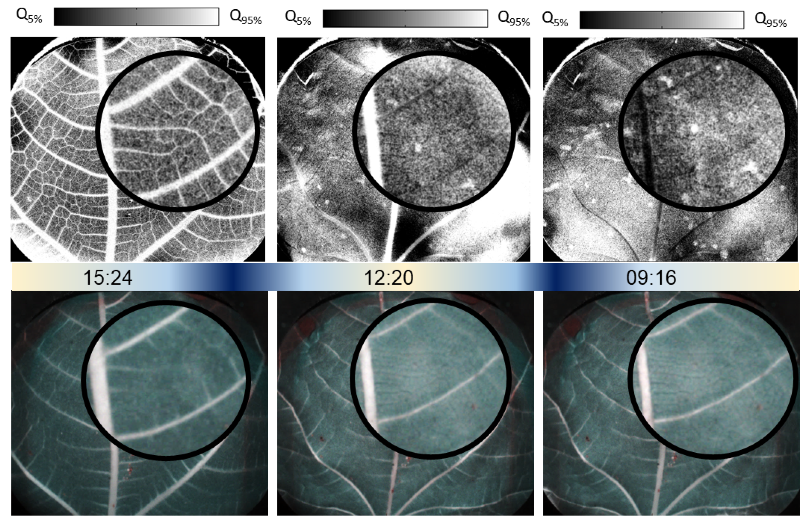
These activity images were arranged in chronological order and formatted into a video sequence, which can be accessed via the link provided in the Supplementary Materials. In Figure 1, we have extracted six key images from this sequence. Note that in this figure and the following ones, examples of edge effects are apparent, where areas of high (or white) activity appear outside the sap flow, contrary to expectations. These occurrences arise from the application of an imperfect mask to the intensities, rendering these values not meaningful.

The first speckle activity image of the video reveals the structuring of sap vessels. As time goes by, the activity signal decreases gradually, starting by vessels of smaller diameter, followed by larger ones until the central vein. In many Fujii index images, large patterns can be observed that appear as positive or negative contrasts relative to the vessel-free regions of the leaf. They are expected to be due to macroscopic movements. As the leaf becomes dehydrated, it often exhibits signs of mechanical torsion, with curling at the edges. These effects are generally easily distinguishable from microcirculation patterns, as they extend over several square centimeters without any detailed pattern. We can also perceive, starting from the fourth index image, small spots of locally higher intensities. In our experience, these local bright spots are correlated with a high degree of dehydration; however, the mechanical origin of these micro-movements remains unknown.

In contrast, the corresponding RGB images do not allow for discrimination of sap activity within the post-cut leaf, nor do they reveal the stress spots observed in the speckle activity images. This highlights the superior sensitivity of speckle activity imaging in detecting subtle changes in sap flow and stress responses in the leaf.

In Figure 2, we compare three Fujii activity indices extracted from the video sequence at different times with the corresponding images in RGB format. The three Fujii activity indices show distinct changes in the leaf, while the RGB images show little difference in leaf structure. The image on the left shows the freshly cut leaf. Many details of the sap circulation network are revealed in the Fujii activity index image, whereas they are hardly perceptible in the RGB image. The image on the middle corresponds to a time of 21 h after cutting. The central vein is still active, but the secondary veins are no longer visible. In the image on the right of Figure 2, the signal has become weak in the central vein. Several spots appear, probably due to dehydration.

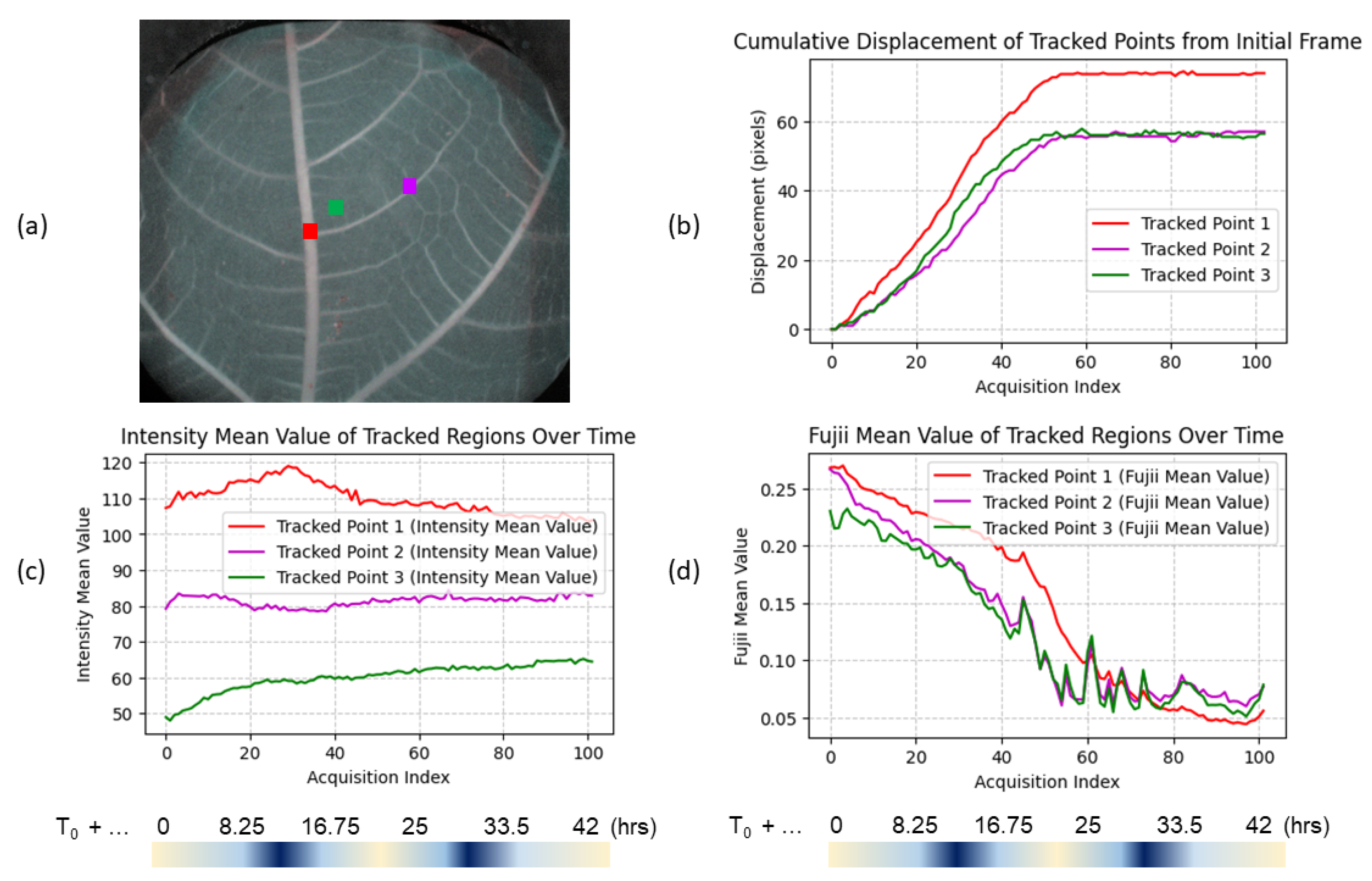
Our primary objective is to qualitatively demonstrate the feasibility of differentiating various speeds of sap flow, assessing the temporal evolution of motion within leaf veins through numerical indices. However, to illustrate the significantly enhanced sensitivity for leaf health tracking achievable through dynamic speckle—a phase-based modality—in comparison to conventional colored intensity imaging, we show these temporal variations in Figure 3 in three key regions of interest (RoIs) on the leaf. The RoIs are located on the central vein (red), a finer peripheral vein (green), and an area outside the vascular structure (purple), with each region sized at 5 × 5 pixels to balance noise reduction and spatial resolution. The selected RoIs were tracked over time using an optical flow algorithm [28], which allowed for the automatic adjustment of coordinates to account for the leaf’s shrinkage over time. The figure shows cumulative displacement in pixels (b), intensity mean values (c), and Fujii index mean values (d) for each RoI across frames. The displacement plot (b) shows that the tracked points exhibit gradual movement over time up to approximately frame 50 (about 24 h after leaf cutting), particularly in the central vein. This movement reflects the natural shrinkage and shifting of the leaf structure after cutting. The intensity mean values from RGB images (c) reveal minimal fluctuations over time, remaining within a 10% variation. In contrast, the Fujii index values (d) demonstrate an earlier and more pronounced decrease, indicating significant changes in sap velocities. The central vein displays the steepest decline in Fujii index values after frame 50, whereas the peripheral vein more quickly reaches a nearly constant value, suggesting differential behavior between the central and peripheral vascular regions.

It should be noted that conventional RGB images and Fujii indices do not convey the same type of information. The intensity in RGB images, currently used for qualitative inspection and assessment of leaf condition, is linked to the radiometric content of the image. It essentially reflects the brightness or pixel value within the visible spectrum. In contrast, the Fujii index is related to the “activity” due to the local micromovements inside the leaf. Finally, while Fujii numerical values provide insights into the relative motion and changes within the leaf, showing promise for velocity mapping of sap flow, they are not yet calibrated in physical units of velocity or displacement. Consequently, these observations are specific to this experiment and represent initial findings that require further study to obtain absolute values of flow velocities.

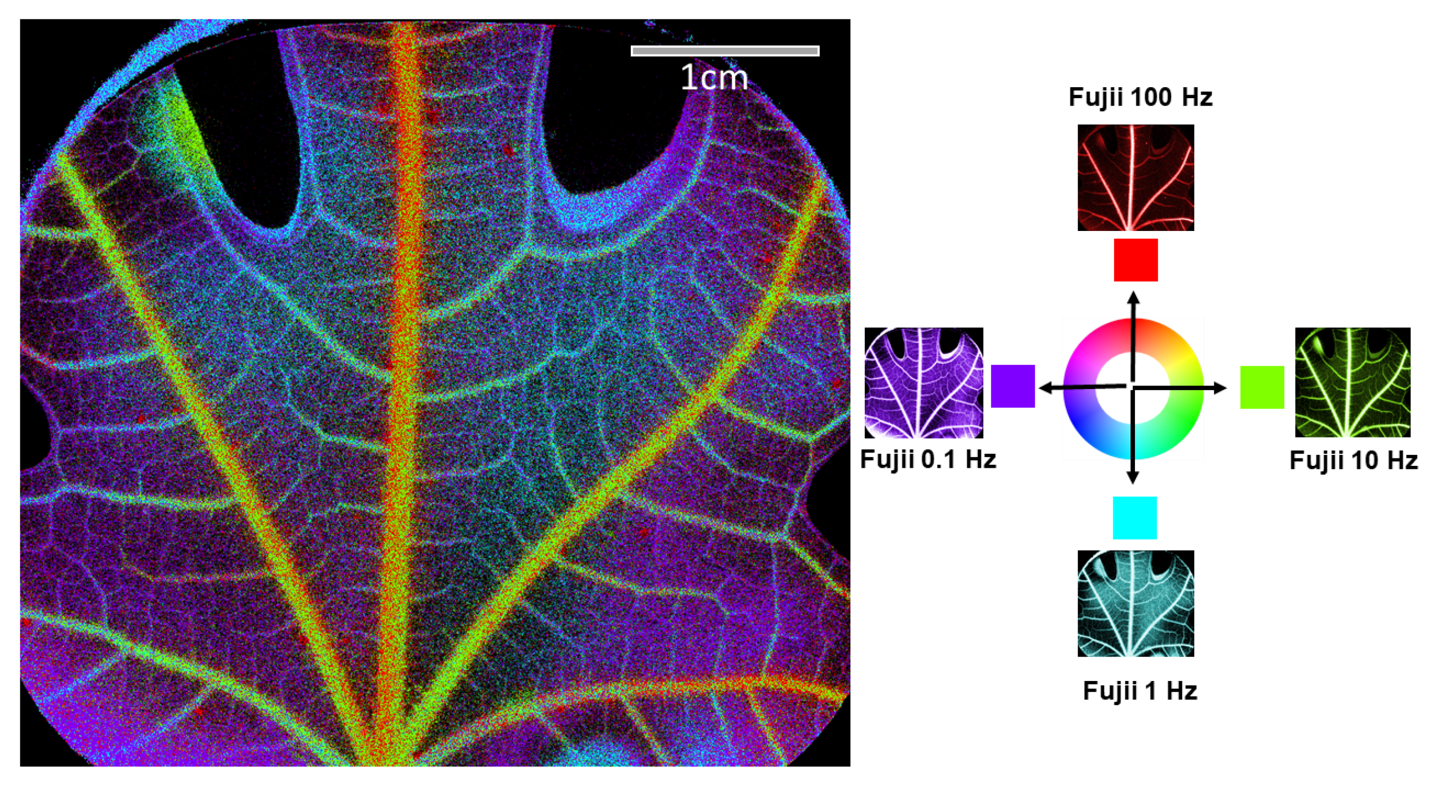
Figure 4 shows different results of activity images obtained on a second freshly cut leaf, using acquisitions of 100 images while varying the acquisition frequencies to 100 Hz, 10 Hz, 1 Hz, and 0.1 Hz. In this series of results, the image acquired at a high frequency (100 Hz) mainly reveals circulation in the central veins, likely because these correspond to the highest sap flow velocities. As the acquisition frequency decreases, the activity signal becomes visible in increasingly finer vessels, enabling a detailed observation of the leaf’s internal dynamics. This is consistent with the fact that sap flow decreases in velocity as it moves through progressively smaller veins in the leaf [16,29]. Consequently, lower acquisition frequencies are required to observe the slower circulation in these smaller veins.

These different images can be combined in a unique color composition for a qualitative analysis. To obtain the composition shown in Figure 5, we encoded our image in the HSV color space: The hue represents the frame rate that achieved the highest Fujii index among the four different acquisition rates, with four distinct hues assigned from the HSV palette. The intensity corresponds to the maximum value of the Fujii index, while saturation is uniformly fixed at 1. This approach allows us to qualitatively verify that acquisition frequencies reveal increasingly finer vessels as frequency decreases.

3. Methods

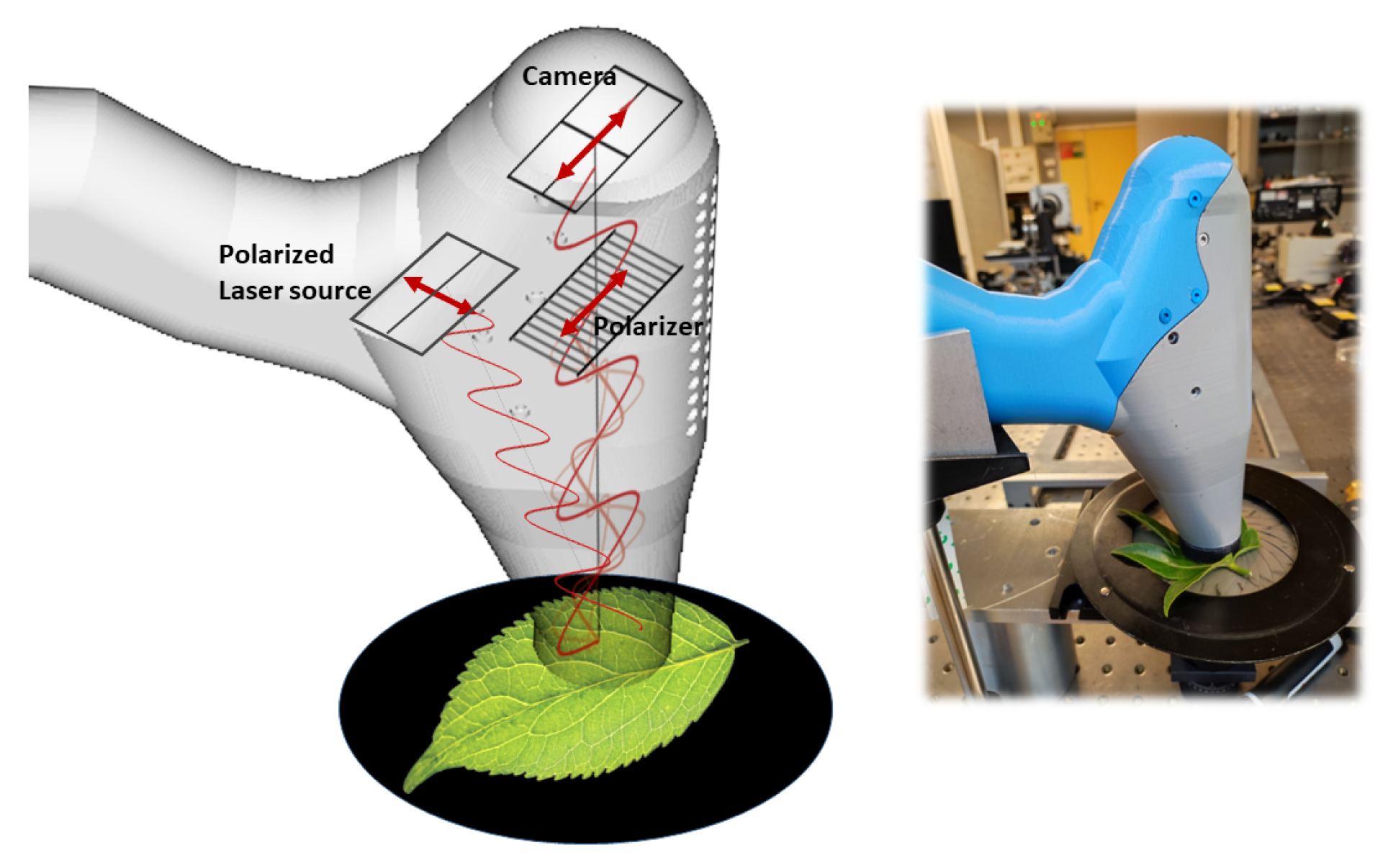
The schematic diagram of the experimental setup is shown in Figure 6. Our experimental configuration is based on an optical technology originally developed and described in [13]. In this technology, the orthogonal polarizer in front of the camera filters out first-order backscattering that conserves mainly the illumination polarization state, thereby emphasizing multiple scattering events occurring deeper in the leaf. The laser used is a lambdamini from RGB Photonics at 785 nm. The converging lens inside the original laser box is taken off and the elliptic shape beam passes through a diverging lens (PCV 6 x-9 FL, NIR coated from Edmund Optics) and a cylindrical lens (CYL 12.7 DIAx-50FL, NIR coated from Edmund Optics) for intensity anisotropy compensation at the object plane. The illuminating field then reaches the sample by propagation in free space. The 3D housing of the imaging system ensures (1) eye safety until the beam diverges sufficiently; (2) that the observed leaf remains in the depth of field; and (3) optical isolation from outside light. In this paper, the field of view is approximately 5 cm by 4.5 cm, represented by a resolution of 1000 by 900 pixels. The dynamic range and noise characteristics of the CMOS camera were rigorously evaluated in prior research [14]. This study presents a comprehensive analysis of the camera’s performance, including assessments of dynamic noise within the operating acquisition frequencies and integration times relevant to our setup, thereby maintaining the consistency and reproducibility of our measurements across similar imaging systems. The continuous laser power of 24 mW passes through diverging optics and illuminates the leaf surface over 20 cm², resulting in a very low power per unit area of approximately 12 W/m², making it completely non-invasive. Since the movements considered are slow compared to the integration time of acquisition, we can freely choose the latter to optimize the radiometric levels. Thus, to remain within the linearity range of the CMOS camera in terms of speckle contrast, as described in [14], we fix a 10 ms integration time in all the experiments. Then, the acquisition rates are varied from 0.1 Hz to 100 Hz. We emphasize that this interframe acquisition delay is the only changing parameter.

The experiments were conducted under controlled laboratory conditions to minimize the influence of external parameters, such as temperature and atmospheric humidity. The two studied leaves were collected from an outdoor fig tree at a height of 1 m under shaded conditions and were positioned immediately after cutting on the laboratory experimental support. The leaves were secured in place using strips, which are visible in the field of view for Leaf 2 in Figure 4. Similarly, the device was fixed to minimize any parasitic movement. After cutting, the leaf was positioned on an absorbent black support to avoid any parasitic backscattering from the support. A spectrometry measurement on the substrate was used to asses that the reflectance of support at 785 nm was less than 0.05.

After recording the data, the Fujii index was calculated at each pixel $\mathbf{x}=(i,j)$ as the contrast between two successive speckle images, averaged over the entire time series [20]:

$$F_1\left(\mathbf{x}\right)=\sum _{k=1}^{N-1}{\displaystyle \frac{|I_k\left(\mathbf{x}\right)-I_{k+1}\left(\mathbf{x}\right)|}{I_k\left(\mathbf{x}\right)+I_{k+1}\left(\mathbf{x}\right)}}$$

(1)

where $I_k$ is the k-th intensity frame and N the number of frames. It is also possible to calculate this index not between consecutive frames, but between frames separated by p ones, thus providing access to Fujii indices calculated for acquisitions at decimated repetition rates:

$$F_p(x,y)=\sum _{k=1}^{N-p}{\displaystyle \frac{|I_k\left(\mathbf{x}\right)-I_{k+p}\left(\mathbf{x}\right)|}{I_k\left(\mathbf{x}\right)+I_{k+p}\left(\mathbf{x}\right)}}$$

(2)

To enable adaptive visualization, we calculate the 5th and 95th percentiles for each coefficient and use these values to rescale the dynamics to a range between 0 and 1.

4. Discussion

Since our study focuses on the circulation of plant sap, a much slower process than blood circulation usually considered in the literature, the speckle patterns appear quasi-static during the integration time required to record a single frame. In this specific context, the traditionally crucial integration time loses its importance as a determining parameter for the final signal. It only influences the total amount of light collected, which must be high enough to ensure a correct signal-to-noise ratio, and sufficiently low to remain in the linearity range of the CMOS camera in terms of speckle contrast.

In our study, however, the repetition frequency emerges as the key parameter. This frequency becomes the main factor influencing the revelation of the signal dynamics, allowing a finer analysis adapted to the slowness of the observed phenomenon. In this context of slow movements, parameters other than the Fujii index, such as signal autocorrelation, are also considered, as demonstrated in [30]. For a discretized signal, this parameter can be calculated using the following expression:

$$r_p\left(\mathbf{x}\right)={\displaystyle \frac{{\displaystyle \sum _{k=1}^{N-p}}{I}_k\left(\mathbf{x}\right)I_{k+p}\left(\mathbf{x}\right)-{\left({\displaystyle \sum _{k=1}^{N-p}}{I}_k\left(\mathbf{x}\right)\right)}^2}{{\displaystyle \sum _{k=1}^{N-p}}{I}_k{\left(\mathbf{x}\right)}^2-{\left({\displaystyle \sum _{k=1}^{N-p}}{I}_k\left(\mathbf{x}\right)\right)}^2}}$$

and we can consider the first-order magnitude $1-r_1$ as the activity index.

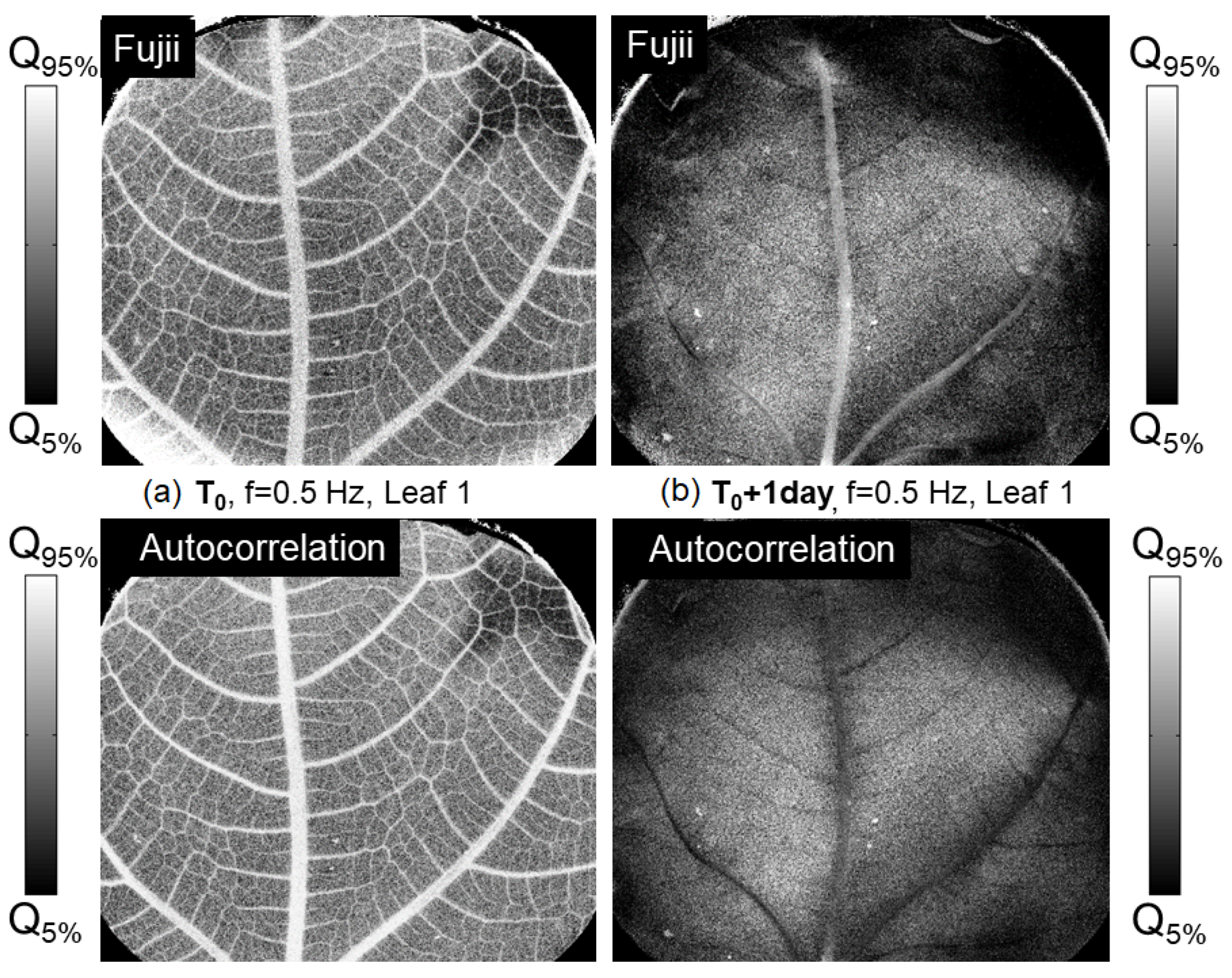
In practice, we calculated the images obtained using the autocorrelation index for all our acquisitions. After adjusting the dynamics of each index separately, the results often turned out to be qualitatively similar. Figure 7 and Figure 8 compare the results obtained from one of the leaves at different moments of the experiment, using either $F_1$ and $1-r_1$ (both of the same order), evaluated from raw images acquired under different conditions. In Figure 7, on the left, we compare the effect of varying the frame rate on the images evaluated using $F_1$ and $1-r_1$ from the data recorded at $T_0$, just after cutting one of the leaves. The Fujii index shows slightly more dynamics in the corners of the image. In the second column (b) of Figure 7, obtained on the leaf 25 h after cutting, the behavior markedly differs: the Fujii index remains higher in the central vein compared to the rest of the leaf, becoming weaker regarding the autocorrelation function. We therefore postulate that the autocorrelation function is less suited to extremely slow movements.

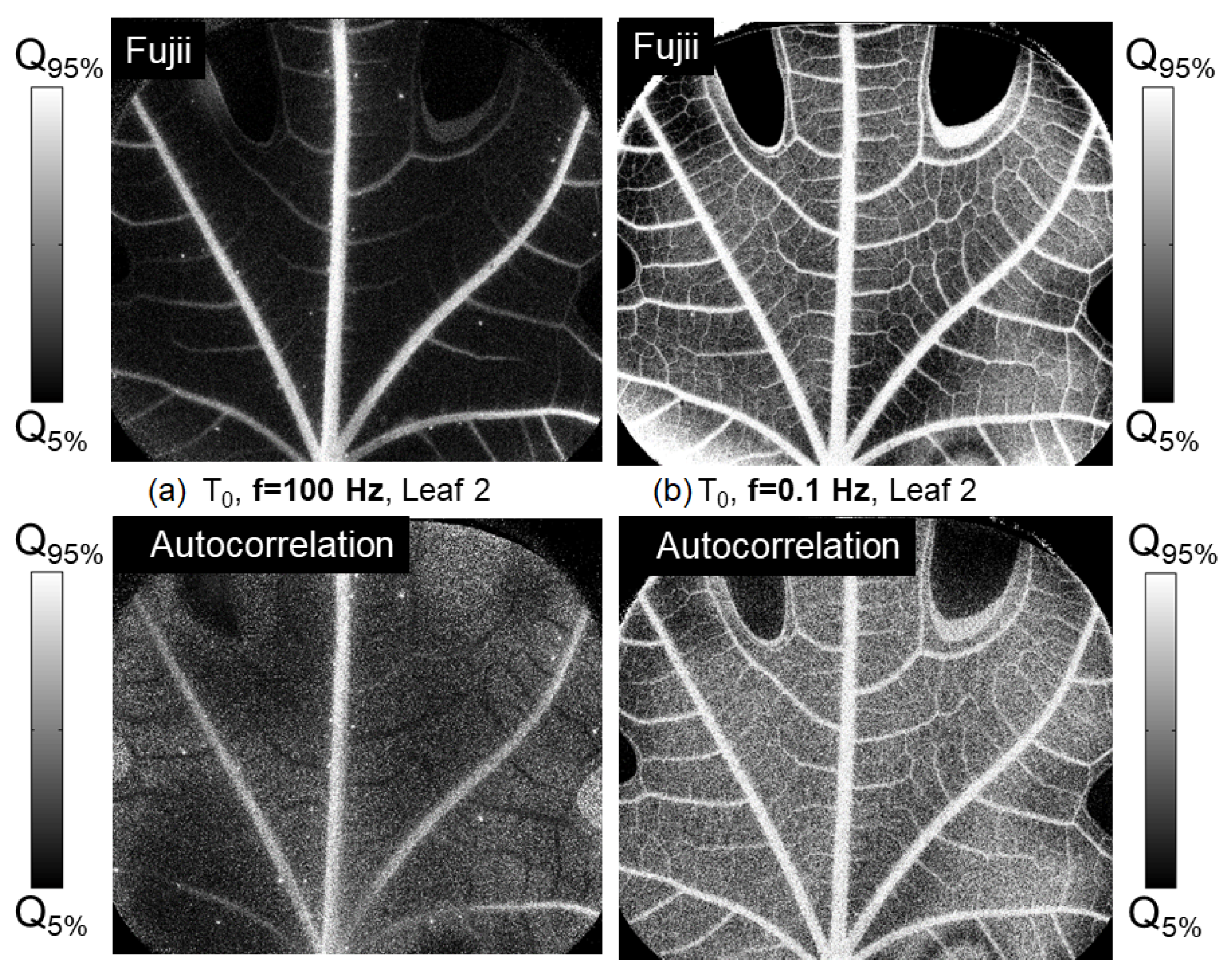
In the first case shown in the first column of Figure 8, for a fast frequency of 100 Hz, the autocorrelation coefficient shows a weaker signal on the small vessels compared with the rest of the leaf. In comparison, the Fujii index shows a greater number of active small vessels. In the second column, comparing $F_1$ and $1-r_1$ from images recorded at 0.1 Hz, the differences between the two statistical parameters are minor. The contrast between the central vein and the background appears slightly more pronounced with the Fujii index compared to the autocorrelation coefficient.

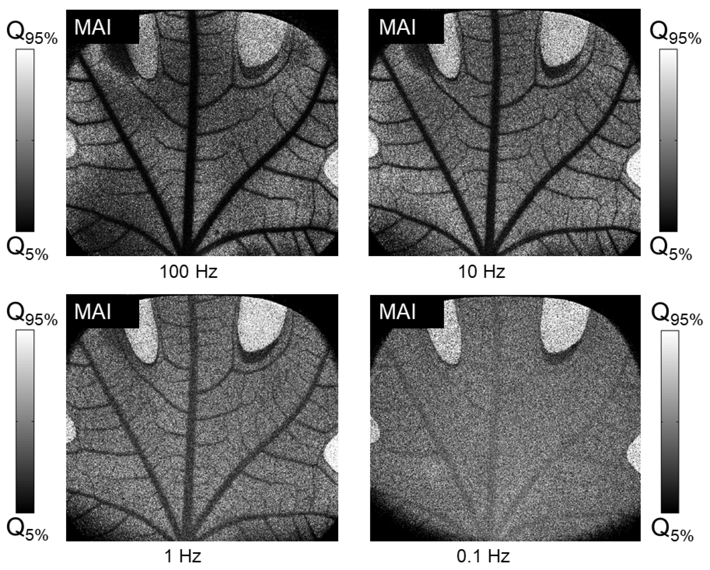
Still regarding the choice of statistical parameter to be estimated, we have shown in practice that temporally calculated speckle contrast is not at completely suited to these dynamics. Indeed, successive acquisitions are highly correlated with each other, and the integration time used is not long enough to include several decorrelation cycles during an acquisition. This makes temporal speckle contrast unsuitable for capturing the slow variations observed in our studies. To further illustrate this, Figure 9 shows images of flow indices, calculated according to the Micro Activity Index (MAI) expression [13]:

$$MAI={\displaystyle \frac{1}{T{C}_t^2}}$$

where T is the integration time and $C_t$ is the temporal contrast of speckle, which can be estimated as follows [10]:

$$C_t{\left(\mathbf{x}\right)}^2={\displaystyle \frac{\frac{1}{N}{\displaystyle \sum _{k=1}^N}{I}_k{\left(\mathbf{x}\right)}^2-{\left(\frac{1}{N}{\displaystyle \sum _{k=1}^N}{I}_k\left(\mathbf{x}\right)\right)}^2}{{\left(\frac{1}{N}{\displaystyle \sum _{k=1}^N}{I}_k\left(\mathbf{x}\right)\right)}^2}}$$

(3)

When the samples are well decorrelated, this expression yields a coefficient proportional to the inverse of the signal decorrelation time, i.e., an activity frequency. However, Figure 9 shows the opposite behavior. This discrepancy highlights the incapacity of temporal speckle contrast in capturing the dynamics we seek to measure in the leaf. At high acquisition frequencies, with highly correlated speckles, speckle contrast is higher in areas of fast flow, resulting in a lower MAI coefficient, contrary to what would be expected. This behavior attenuates as the acquisition frequency decreases. However, even reducing the frequency to 0.1 Hz does not completely reverse the trend: it only homogenizes the values between fixed and moving zones, making the final result of little use. Moreover, at this frequency, the contrast between leaf tissue and sap flow is notably poor, indicating that temporal speckle contrast fails to differentiate these regions effectively.

Finally, we can question the origin of the signal associated with the movement of sap, which is typically a light, transparent and weakly scattering medium. One possible explanation for the observed speckle patterns is the contribution of multiple scattering events, which may occur even in weakly scattering media due to structural inhomogeneities within the sap. These inhomogeneities could arise from microscopic particles or cellular structures within the sap that scatter light. Thus, while sap is transparent at the macroscopic scale, it may still contain enough scattering elements to support speckle formation when observed at the wavelength scale. A second hypothesis is that sap flow slightly modifies the position and diameter of the vessels. In this case, the extreme sensitivity of speckle to wall displacements of the vessels may explain the observed dynamics and subsequent decorrelation phenomena. However, we currently have limited data on the precise mechanisms behind speckle generation within sap-filled vessels, so we are cautious in drawing definitive conclusions at this stage.

5. Conclusions

We have developed an imaging method that allows visualization of leaf activity through its sap microcirculation, using orthogonal polarization dynamic speckle imaging. Unlike medical applications of dynamic speckle imaging where speckle decorrelation is rapid and movement can be captured from a single image with temporal estimation from multiple decorrelated frames, our approach addresses the specific challenge of low velocities in leaves where successive speckle images are not decorrelated. Instead, we seek parameters that reveal the rate of decorrelation, such as the Fujii index, which has proven to be the most effective in our data compared to other criteria, such as the autocorrelation function of intensity.

Our main finding is that by lowering the acquisition frame rates, we can capture increasingly fine details of slower velocities. Since sap circulation speed is correlated with the size of veins, adjusting these repetition rates has allowed us to produce images with unparalleled spatial resolution. This novel approach enables the mapping of various sap circulation speeds. Thus, calculating the Fujii indices for different frame rates or periods provides a new descriptive space for analyzing these dynamics.

We have tracked the evolution of these microcirculation patterns from the moment a fresh leaf is cut until the signal ceases. The results have, for the first time, demonstrated that the vitality of a leaf can be directly tracked by dynamic speckle signal, with the microcirculation image providing much greater informational richness compared to static RGB images, which can neither describe temporal physiological processes nor detect early leaf senescence that induces spatial changes in the vessel network activity.

The potential advantages of our approach over existing methods are many. This full-field device promises high spatial resolution, enabling sap flows to be visualized at a fine scale for an entire leaf. Additionally, dynamic speckle provides sufficiently high temporal resolution to capture rapid variations in sap flow.

Our results may be of significant interest in agriculture for studying plant vitality and understanding the impact of environmental conditions and stress factors on plants in real time. Extending the method to allow in situ monitoring of living leaves without the need for cutting would significantly enhance its applicability. Future studies are already planned to explore this possibility, aiming to adapt the setup for non-invasive monitoring directly on intact plants. Additionally, these studies will deepen the interpretation of changes in the Fujii index by examining potential correlations with specific biomarkers indicative of plant health. Our goal is to identify and quantify these markers, enabling the method to provide more robust and biologically meaningful information about the physiological status of plants. The compactness of the system facilitates in situ work; however, the external environment—such as wind, vibrations, and intense light—will necessitate a new design tailored to these conditions.

Further research will also be necessary to better understand the physics of the processes responsible for the occurrence of dynamic speckle due to sap flow in plant tissues and the conditions that contribute to speckle generation in these biological vessels. We plan to explore this aspect in more depth to clarify the origins of speckle patterns in such weakly scattering media.

• Supplementary Materials: The video of the sap decline is available at https://youtu.be/xUzMFFnhxqk (accessed on 25 July 2024).
• Material availability
  This study did not involve specialized physical materials; all results were obtained through theoretical analysis and computational simulations using standard software tools.
• Code availability
  The drive link to data and notebook can be accessed at http://bit.ly/3zSHkgn (accessed on 25 July 2024). This link provides access to a Google Colab Python notebook designed to analyze the sap flow data from the leaf cut experiment. The notebook includes all the necessary code to process the data and reproduce the results presented in this article.