Accurate, Fast, and Non-Destructive Net Charge Measurement of Levitated Nanoresonators Based on Maxwell Speed Distribution Law

Abstract

Nanoscale resonant devices based on optical tweezers are widely used in the field of precision sensing. In the process of driving the nanoresonator based on the Coulomb force, the real-time, precise regulation of the charge carried by the charged resonator is essential for continuous manipulation. However, the accuracy of the existing charge measurement methods for levitated particles is low, and these methods cannot meet the needs of precision sensing. In this study, a novel net charge measurement protocol for levitated particles based on spatial speed statistics is proposed. High-precision mass measurement based on Maxwell’s rate distribution law is the basis for improving the accuracy of charge measurement, and accurate measurement of net charge can be achieved by periodic electric field driving. The error of net charge measurement is less than 7.3% when the pressure is above 0.1 mbar, while it can be less than 0.76% at 10 mbar. This proposed method features real-time, high-precision, non-destructive, and in situ measurement of the net charge of particles in the medium vacuum, which provides new solutions for practical problems in the fields of high-precision sensing and nano-metrology based on levitated photodynamics.

1. Introduction

As a technology using laser beams to capture and manipulate atoms or nanoparticles, optical tweezers in vacuum can better isolate the external environment [1], achieving better signal-to-noise ratio [2] and detection sensitivity than conventional optical tweezers [3]. Furthermore, accurate measurements of various physical parameters [4,5,6,7] are realized by the use of optical tweezers in vacuum, which has become an important physical platform for high-resolution mechanical detection [8], quantum state simulation, manipulation [9], and collapse model testing [10]. Precision measurement methods based on optical tweezers in vacuum is applied in detecting Casimir force [11], nonlinear optics [12], submicron scale gravitational behavior [13], dark matter interaction [14], the quantum Hall effect system [15], etc. Significant progress has been made in some new physical phenomena, and this progress has gradually expanded in application fields such as quantum information science [16], astronomical space research [17], and biomedicine [18,19].

The application of optical tweezers in the field of precision sensing is inseparable from the Coulomb force, so the net charge is one of the most important parameters in levitated opto-mechanics. Based on the charge characteristics of levitated particles, electric field feedback control can be used to obtain the electrostatic cooling temperature [20], measure basic physical quantities [21], and improve the levitating stability of particles [22]. Due to the reliance on electric field stability in the process of physical quantity measurement, the accurate calibration of the net charge has become a top priority. Traditional net charge measurement usually requires physical contact. For example, in 1923, Robert Millikan [23] measured the single charge e through an oil drop experiment. The Zeta potential method [24,25] can evaluate the charge properties of particles, colloids, and interfaces in liquid media. Electric force microscopy (EFM) [26] can measure the charge distribution on the sample surface on a solid substrate. However, the existing methods are basically continuous statistics of the charge of groups, not the single particle. Furthermore, the above method cannot be applied to the field of optical tweezers in vacuum due to the limitation of the pressure range.

Optically levitated nanoparticles driven by an external time-harmonic electric field have been reported several times. For example, Hempston et al. [27] used charged nanoparticles for force sensing. Zhu [28] also combined a periodic electric field drive with feedback cooling to achieve high-sensitivity detection of three-dimensional electric fields. Ricci [29] used periodic external electric fields to achieve precise mechanical measurements. However, the net charge usually needs to be re-measured when the experimental state changes. Current methods for directly measuring the net charge of particles in levitated optical traps mainly rely on the step-ladder method, using ultraviolet discharge [30] or high-pressure ionization [31] to control the net charge change of particles. This process is not only accompanied by large randomness, but also affects the levitation stability.

In fact, the existing net charge method based on the time-harmonic electric field has a large error. For example, Hempston [27] applied DC and AC electric fields to a metal probe near a trapped particle, and the net charge calculation accuracy was about 10% at high vacuum. Frimmer [32] designed a simple net charge control and measurement method. Subsequently, Wang used this method to measure the net charge with an error of even higher than 20% [33]. This was mainly due to the uncertainty of the particle mass. The lack of knowledge of particle mass seriously affects the accuracy of calibration, thus limiting its application in sensing and measurement.

Here, we propose and validate a fast measurement of the net charge of nanoparticles based on the Maxwell speed distribution law. Our results are superior to those obtained with conventional discrete charge calibration. The measured mass error is as low as 4% and the charge error is as low as 0.7%. A careful error estimation is performed to evaluate the final charge uncertainty. Our proposed technique allows real-time measurement of the net charge in the vacuum range above 0.1 mbar, and the net charge measurement accuracy is improved by more than one order of magnitude [33].

2. Theory

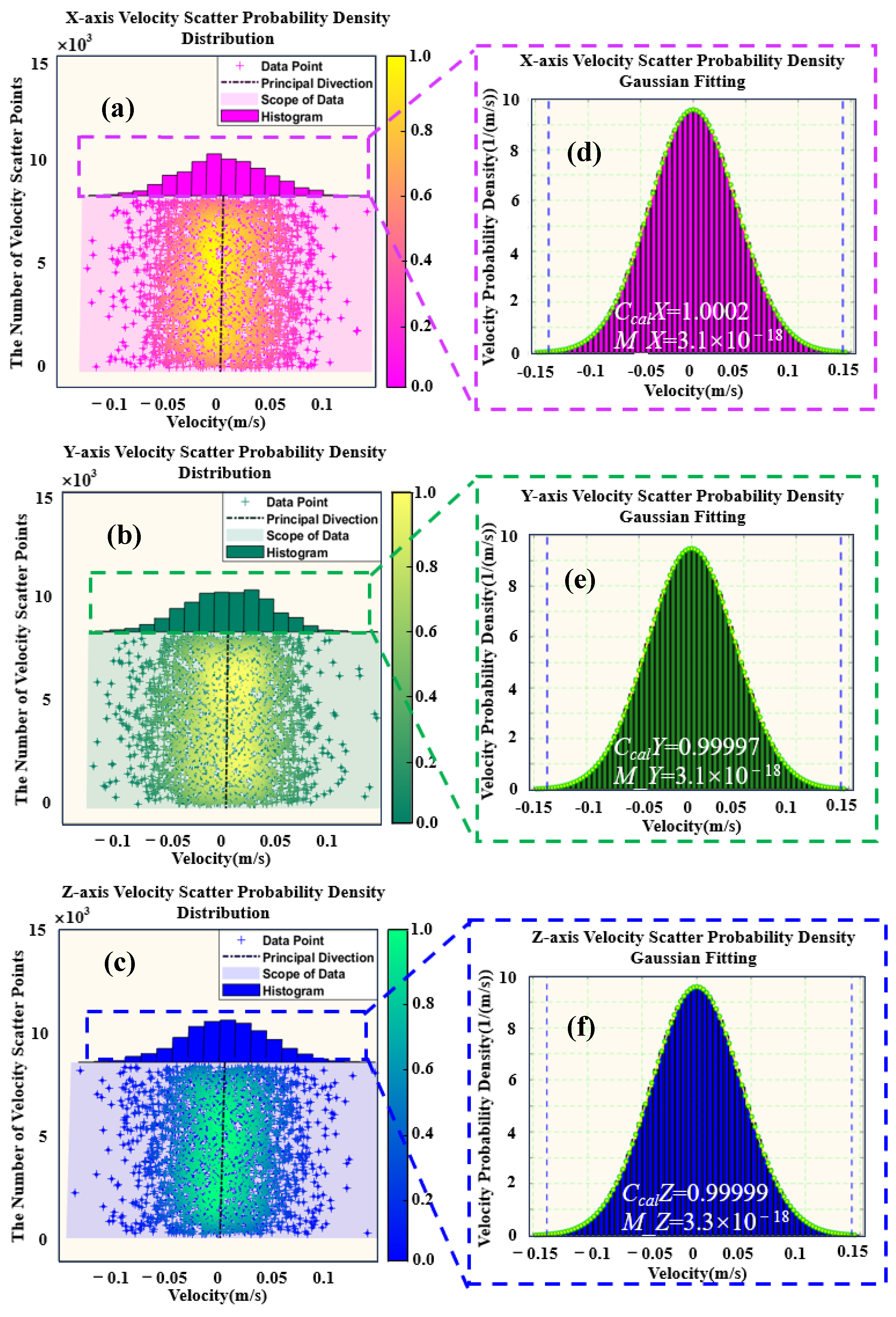
2.1. Derivation of Maxwell Speed Distribution Law Based on Levitated Nanoscale Resonators

When the gas is in equilibrium, the number of molecules inside tends to infinity, and the probability distribution of the speed follows certain statistical laws. In 2010, Li [34] directly measured the instantaneous speed of Brownian particles and verified the Maxwell speed distribution law. It is a probability density function that describes the speed of microscopic particles at a certain temperature, and it can be regarded as a statistic of the spatial speed of the particles. It is known that each vector velocity component of the particle in the three-dimensional direction conforms to an independent normal distribution with an expectation of 0 and a standard deviation of a:

$$\begin{array}{l}{v}_{x(y,z)}~N(0,a^2)\\ v=\sqrt{v_x^2+v_y^2+v_z^2}\end{array}$$

(1)

In statistical physics, the three-axis vector velocities, $v_x$, $v_y$, $v_z$, are considered to be isotropic and independent of each other. Usually, we are not interested in the one-dimensional position distribution, but instead in the probability distribution of the particle’s spatial speed v. The probability of a particle’s one-dimensional velocity [35] can be expressed as a Gaussian distribution $g(v_x^2)=\sqrt{{\displaystyle \frac{m}{2\pi k_{B}T}}}\exp ({\displaystyle \frac{-m{v}_x^2}{2k_{B}T}})$. So, the final space vector velocity v_velocity can be summarized as follows:

$$f(v_{velocity})=a^{1/2}·\exp [-\pi a{(v_{velocity}/c_{calib\_x,y,z})}^2]$$

(2)

Obviously, the expression is a normal curve with symmetrical distribution, and the probability density function of the vector velocity v_velocity satisfies the Maxwell–Boltzmann distribution, where $a=m/(2\pi k_{B}T)$ is the target result containing the fitting quality, and c_{calib_x,y,z} is the update coefficient of the three-axis velocity, which can achieve calibration of quality by increasing the number of iterations. The particle in the optical trap performs simple harmonic motion around the focus. Only the magnitude of its velocity is needed, not the direction. At this time, the Maxwell speed distribution law for the scalar v_speed can be expressed as [36]

$$f(v_{\mathrm{speed}})=a^{3/2}·4\pi {(v_{\mathrm{speed}}/c_{calib})}^2·\exp [-\pi a{(v/c_{calib})}^2]$$

(3)

For a single particle, f(v_speed) represents the probability of being near a unit interval of speed v during free space motion, and its probability density distribution curve is not axisymmetric. In subsequent calculations, we substitute the three-axis motion information v and other prior knowledge into Equation (7) for parameter fitting to obtain the final mass information [33].

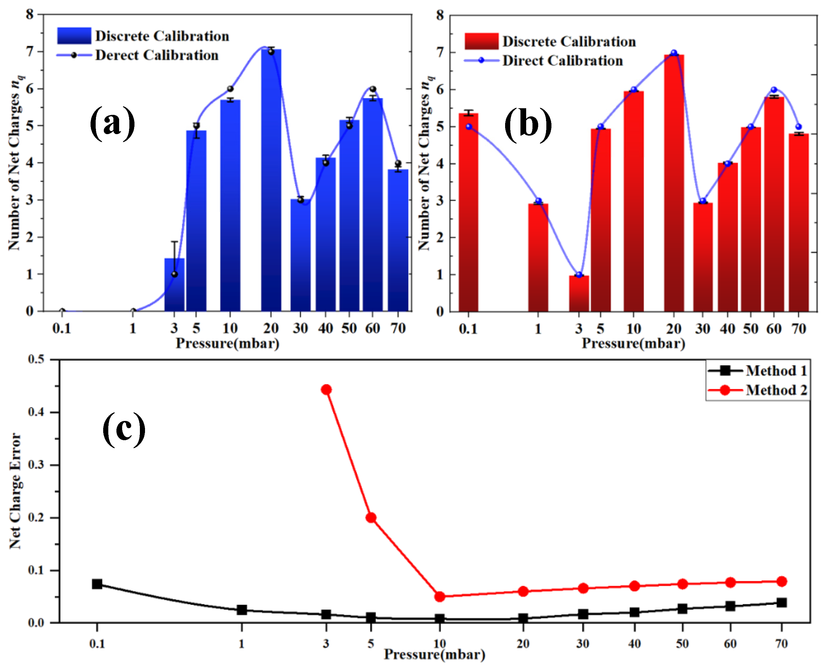
2.2. Electrical Drive Response and Net Charge Measurement

In order to describe the relationship between the target position x of the particle and other random variables changing with time $\tau$, the Langevin equation of one-dimensional random Brownian motion can be used [37]:

$$m{\displaystyle \frac{d^{2}x}{d{t}^2}}+\gamma {\displaystyle \frac{dx}{dt}}+m{\Omega }_0^{2}x=F_{rand}(t)/m+F_{dr}/m$$

(4)

where m is the particle mass and ${\Omega }_0$ is the eigenfrequency. $\gamma =m\Gamma$ is Stokes viscosity coefficient, $\Gamma$ is the damping rate, and $F_{rand}$ represents the external random force caused by thermal noise. In the AC electric field with a driving frequency of ${\omega }_{dr}$, the driving electric field strength is $E=E_0\cos ({\omega }_{dr}t)$. The electric driving force equation with a particle net charge number n_q is $F_{dr}=n_q{q}_e{E}_0\cos ({\omega }_{dr}t)$. At air pressure p > 10 mbar, the system is in thermal equilibrium. The total power spectral density (PSD) of the thermally driven mechanical resonant system under electric driving can be expressed as [28]

$$\begin{array}{l}{S}_x(\Omega )=S_x^{th}(\Omega )+S_x^{dr}(\Omega )\\ ={\displaystyle \frac{4k_{B}T\Gamma }{m[{({\Omega }_0^2-{\Omega }^2)}^2+{\Omega }^2{\Gamma }^2]}}+{\displaystyle \frac{F_{dr}^2}{2m^2}}{\displaystyle \frac{\tau \sin c^2[(\Omega -{\Omega }_{dr})\tau ]}{{({\Omega }_0^2-{\Omega }^2)}^2+{\Omega }^2{\Gamma }^2}}\end{array}$$

(5)

where k_B is the Boltzmann constant, T = 300 K is equivalent to the ambient air temperature of the particle, $S_x^{th}(\Omega )$ is the thermally driven PSD, $S_x^{dr}(\Omega )$ is the electrically driven PSD, and dynamics x(t) is observed for a time $\gamma =2\tau$. $S_x(\Omega )$ is related to the experimentally measured $S_v(\Omega )$ through the calibration factor C_cal, and the corresponding relationship is as follows:

$$S_v(\Omega )=C_{cal}^2·S_x(\Omega )$$

(6)

In the experiment, $S_v(\Omega )$ can be directly measured, and C_cal converges through multiple fitting calibrations. The damping rate $\Gamma$ and the eigenfrequency Ω₀ of the X axis are obtained by fitting the Lorentz curve to $S_v^{th}(\Omega )$. Similarly, for a driving signal with a known frequency ${\Omega }_{dr}$, the power spectrum density of the driving signal can be obtained. The final net charge q_e can be calculated by the ratio $Rs={\displaystyle \raisebox{1ex}{$S_x^{dr}({\omega }_{dr})$}\!\left/ \!\raisebox{-1ex}{$S_x^{th}({\omega }_{dr})$}\right.}={\displaystyle \raisebox{1ex}{$S_x-S_x^{th}$}\!\left/ \!\raisebox{-1ex}{$S_x^{th}$}\right.}$ of the PSD of the electric field driving part to the thermal driving part, and the final charge is as follows:

$$n_q=\sqrt{{\displaystyle \frac{8k_{B}T\Gamma R_{s}m}{q_e^2{E}_0^2\gamma }}}$$

(7)

Because the net charge n_q is an integer, the exact charge number can be obtained based on rounding. The main measurement error comes from the uncertainty of the particle mass m. Measuring m accurately ensures that the error in the charge is minimized.

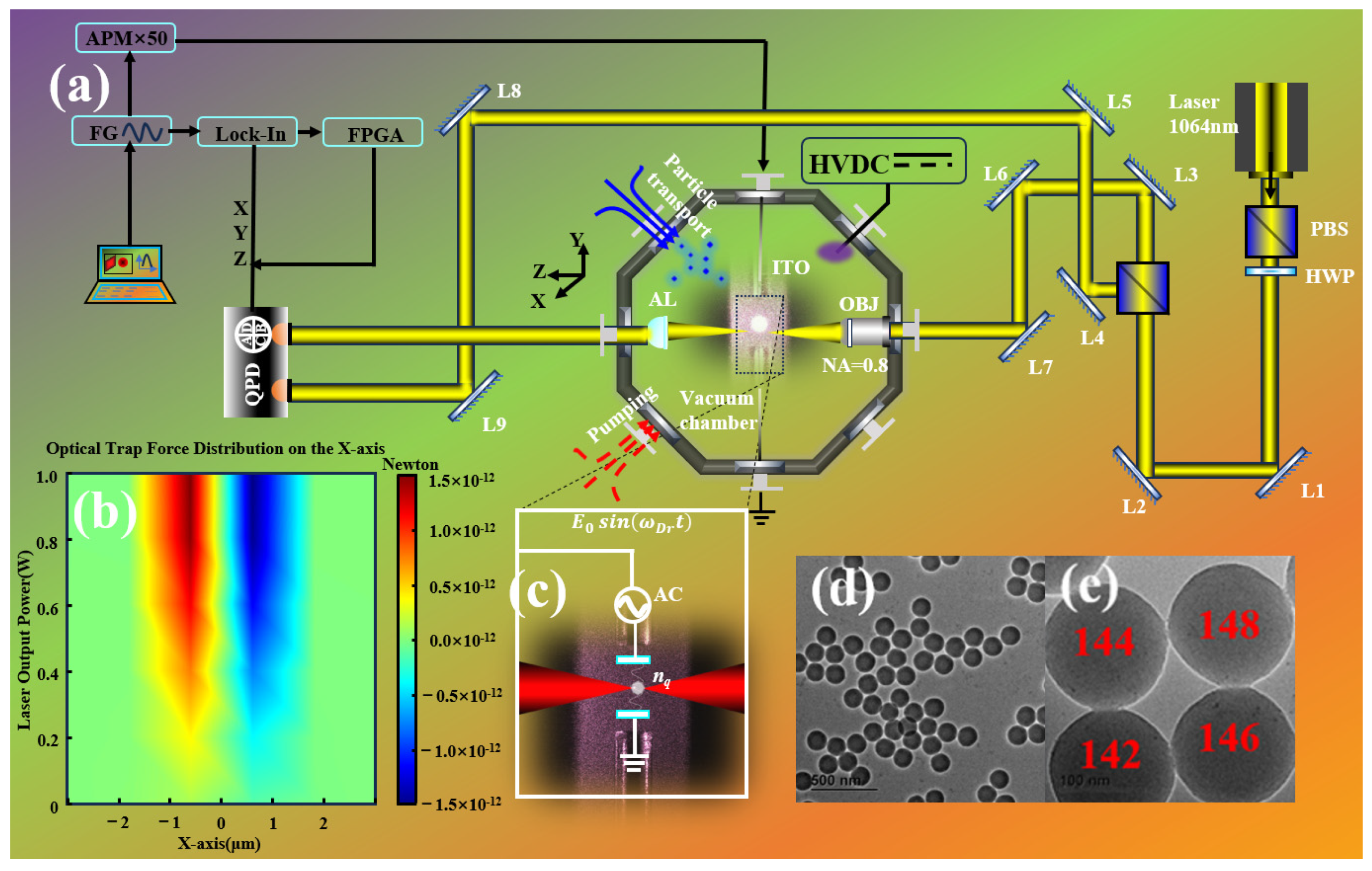
3. Externally Driven Net Charge Measurement Device for Levitating Particles

Based on the understanding of Maxwell speed distribution law and electric field sensing method, we designed the optical levitation device as shown in Figure 1a. The device enables simultaneous mass measurement and its subsequent net charge measurement. The propagation direction of the light beam is defined as the Z axis, and the X axis corresponds to the polarization direction of the captured linear polarized light. An optical levitated particle can eventually be regarded as an extremely sensitive sensor. The force of light acting on the particle produces the displacement, which can be obtained by the signal difference between the scattered light and the reference light (refer to the two light signals incident on the QPD in Figure 1a). The scattered signal is collected by an aspheric lens (AL). The microscope objective (OBJ) with a numerical aperture NA = 0.8 is selected to ensure large capture efficiency for the light trap. Figure 1b is a simulation diagram of the optical force mapping between the laser power P₀ and the axial position x. In this illustration, the positive optical trap force indicates that it is opposite to gravity. A sufficiently large optical trap force allows the particle to overcome the effects of gravity (the particle gravity is approximately 3.5 × 10⁻⁷ N) and random forces. In order to ensure a sufficiently high capture efficiency, the incident power is set to P₀ = 800 mW. The quadrant photodetector (QPD) realizes real-time monitoring of the three-axis displacement. The motion information in the spatial direction is synchronously collected by the data acquisition module, and the position signal is output to the computer for particle parameter fitting processing. A pair of parallel plates in the vacuum cavity generates a uniform electric field around the light trap, as shown in Figure 1c. A high voltage direct current (HVDC) power supply ionizes the air to make the particles carry random charges [29], providing conditions for subsequent net charge measurement. Silica nanoparticles are used as the most basic sensing unit, and their morphology and size are shown in Figure 1d,e (Micronano, d = 150 ± 8 nm), which intuitively proves that the actual diameter of the particles used in the experiment basically meets the manufacturer’s nominal range.

The dispersed single spherical silica particles are diluted 1000 times in isopropanol and atomized into a vacuum chamber at normal pressure. When the particles are captured by the light trap, the pressure is reduced to p < 10⁻² mbar to cause the particles to lose hydroxyl groups [38]. In theory, the mass of the dehydroxylated particles no longer changes with air pressure.

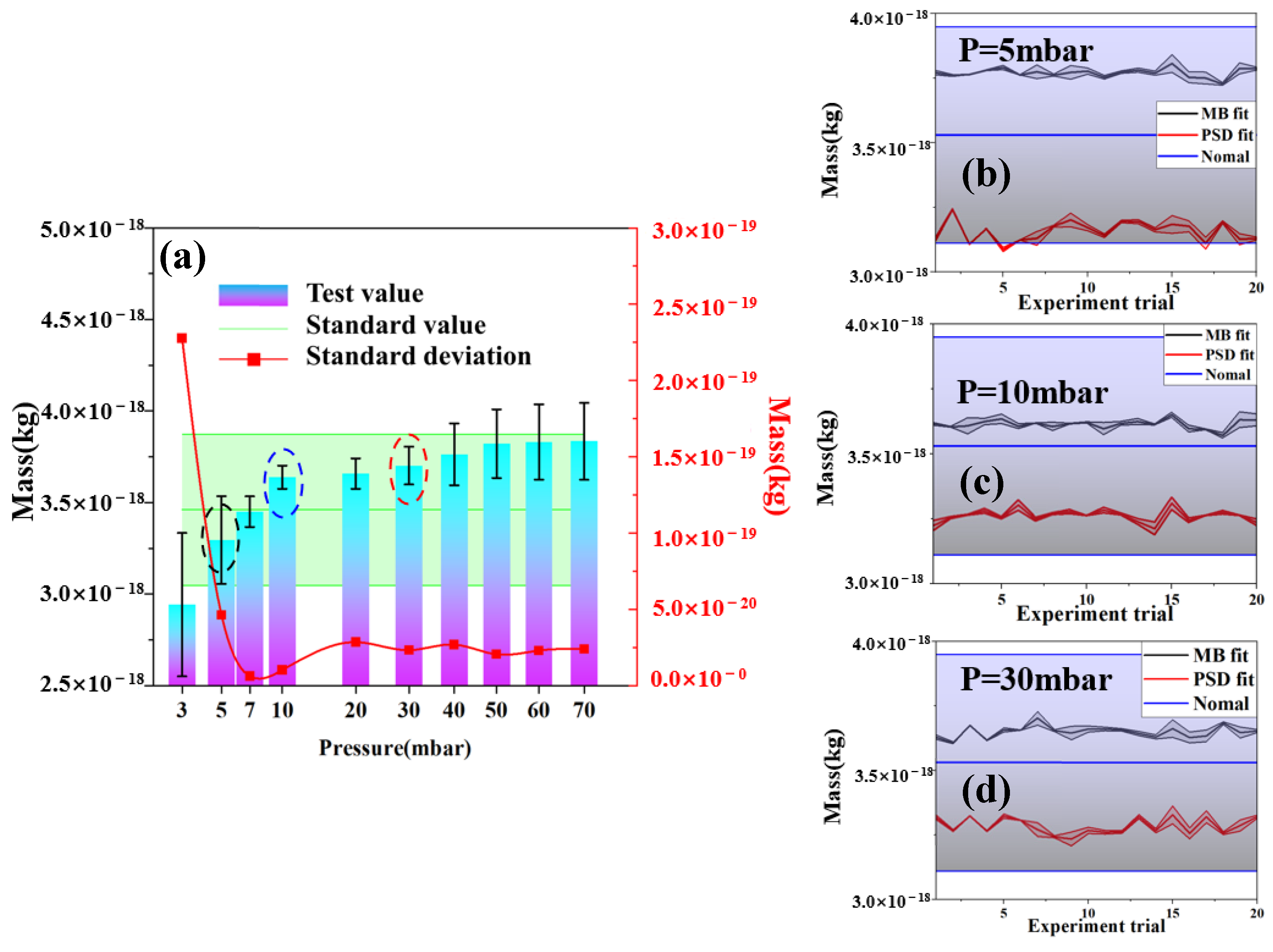
4. Experimental Results Display and Error Analysis

The scattered light signal of the particle is collected synchronously in three axes, and the PSD curves are obtained by filtering and fitting. As shown in Figure 2a, the three-axis natural frequencies under p = 10 mbar are ${\Omega }_x$ = 179.4 kHz, ${\Omega }_y$ = 202.3 kHz, and ${\Omega }_z$ = 55.9 kHz. The pressure p = 10 mbar is selected because the particle motion is in the linear range at this time, and no additional nonlinear compensation for the displacement is required. The trajectory information of the particles in thermal equilibrium is collected for a long time, and suggests equipartition of the potential energy amongst all the degrees of freedom to achieve accurate measurement of the parameters in equilibrium [39]. Figure 2b,c shows the error curve of the corresponding relationship between the thermal noise and the air damping rate with the change of air pressure obtained by Lorentzian fits, where $S_v^{th}(\Omega )$ = 8.502 ± 0.053 V²/Hz, $\Gamma$ = 6.25 ± 0.01 kHz with p = 10 mbar. The conversion relationship between the voltage signal V and the displacement x obtained by fitting the PSD can be expressed as $x=C_{calib}·V$ [40], where $C_{\mathit{calib}}=\sqrt{{\displaystyle \frac{k_{B}T}{m{\Omega }_0^2\langle V^2\rangle }}}$ is only a preliminary result. Later, multiple fitting iterations will be performed based on the Maxwell speed distribution law and the calibration process will be demonstrated.

In order to achieve the fitting based on the Maxwell speed distribution law, the velocity statistics of the particles in the three-dimensional direction were obtained at p = 10 mbar. The simple harmonic oscillation motion of the particles near the optical trap is accompanied by the reciprocating change of velocity. The particle velocity distribution at different times can be understood as a model similar to the electron cloud, as shown in Figure 3a–c. The density of these scattered points represents the velocity distribution of the particles at different times, which is obtained based on the differences in particle position x and sampling frequency. The velocity distribution on the X axis gradually decreases in density from the origin to both sides, with a clear Maxwell–Boltzmann distribution trend.

We performed Gaussian fitting on the filtered data of the three-axis velocity. According to Equation (6), we need to input the preset mass of the particle and the temperature of the surrounding gas. The particle mass is calculated based on the manufacturer’s data ($m=3.53\pm 0.42fg$, $\rho =1973\pm 267kg/m^3$), and the iterative fitting parameters of the three-axis velocity probability density are obtained according to Equation (6), as shown in Figure 3d–f. The three-axis velocity is iterated 20 times by the Maxwell–Boltzmann distribution fitting. $C_{cal}X(Y,Z)$ is the update coefficient of the Vm coefficient of the three axes, representing the correction of the original velocity. M_X (Y, Z) represents the three-axis mass fitting results obtained according to the Maxwell–Boltzmann distribution, which only represents the particle mass derived from the one-dimensional motion in a certain direction.

Figure 4 shows the iterative process of the velocity update in three orthogonal directions. During the iteration process, the confidence interval r² > 90% is required to ensure the credibility of the data. Vm_X(Y, Z) is the Vm coefficient of the three-axis velocity, which represents the calibration process of the Maxwell–Boltzmann distribution for the original velocity acquisition data. The Vm coefficient calibration coefficient $C_{cal\_x(y,z)}$ on the three axes gradually approaches 1 with the number of iterations and the particle velocity distribution trend tends to converge, ensuring the stability of subsequent mass calculations.

The particle’s scalar speed, denoted as v_speed, is determined by taking the square root of the velocity correction components $v_{x(y,z)}$ in three orthogonal directions, according to Equation (1). The resulting speed probability density distribution is shown in Figure 5a,b, exhibiting asymmetrical scatter points characteristic of the Maxwell speed distribution law. By calculating the probability density of the particle’s speed at different times and fitting it with Equation (7), we can determine the mass of the particle. Figure 5c,d is the speed probability density histogram based on the Maxwell speed distribution law fitting, showing the parameter results of the first fitting and 20 fittings after 26 s of simultaneous acquisition of three-axis data. As more fittings are conducted, the speed update coefficient $C_{cal}V$ gradually converges towards 1, leading to an estimated final particle mass of approximately 3.6 × 10⁻¹⁸ kg.

In the pressure range of 3 mbar~70 mbar, multiple groups of mass measurements were performed continuously for a long time to find the pressure value p at which the particle mass is most accurate based on the Maxwell speed distribution law. In order to reduce random errors, 20 groups of repeated tests were performed at each pressure. The final mass measurement results are shown in Figure 6a. The blue–purple gradient bar graph represents the final mass result of the particle after the Maxwell speed distribution law fitting. The black error bar is the mean absolute error (MAE) under multiple measurements. The MAE of the mass is the smallest when p = 10 mbar, indicating that the mass measurement accuracy is the highest at this pressure. The green curve and its coverage area represent the standard mass range given by the manufacturer. It can be seen that in the pressure range of 5 mbar–30 mbar, the mass measurement value and its MAE are within the allowable error range, which can also be proven through known theories. The energy equipartition theorem has the best application range near p = 10 mbar, and its reliability decreases with the change of pressure. The red dotted line represents the standard deviation of the mass measurement, which measures the distribution of the test data deviating from the sample mean, indicating that the data are more concentrated when p = 10 mbar. In Figure 6b–d, the new method is compared with common mass measurement methods [8]; the mass of the same particle under experimental pressure was measured 20 times. The final results show that the new method has the best quality detection results for 150 nm diameter particles at 10 mbar, and the final measurement result is M_MB = 3.65 × 10⁻¹⁸ kg. The mass uncertainty is 6.8% at 5 mbar, 5.8% at 7 mbar, 4% at 10 mbar, 6% at 20 mbar, and 8.5% at 30 mbar.

Figure 7a shows the details of the electric field parameters. An electric field of $E(\tau )=E_0\cos ({\omega }_{dr}\tau )$ was applied to the flat electrode, and the output frequency was f_dr = 160 kHz. As shown in the black curve in this figure, $Rs={\displaystyle \frac{S_v^{dr}({\omega }_{dr})}{S_v^{th}({\omega }_{dr})}}={\displaystyle \frac{S_v({\omega }_{dr})-S_v^{th}({\omega }_{dr})}{S_v^{th}({\omega }_{dr})}}\simeq 80$, and the thermal noise of the bottom blue curve is less than 3 × 10⁻¹³ V²/Hz. Figure 7b shows the step measurement charge method commonly used in the field of optical tweezers in vacuum. Multiple random charging processes can find the minimum step change e, and then determine the net charge number n_q of the particle based on the multiplier relationship. Since the number of charges is an integer, the measurement error of the step-ladder method in the case of low charge is 0, which can be used as the true value to form a control group with the new method. However, the step-ladder method has obvious defects. The air pressure must be between 1 mbar and 5 mbar to achieve a large range of charge adjustment, otherwise the step change is not obvious. In addition, the change of charge is a random process, which will destroy the state of the existing charge and cannot achieve real-time measurement in the levitate system.

Several sets of experiments were conducted on the same device at the same pressure in the pressure range of 0.1 mbar to 70 mbar, and the new method was compared with previous studies to demonstrate its advantages in measurement. Figure 8a shows the net charge n_q calculated by previous work [33]. The charge error at 10 mbar is about 5%, and the error at 70 mbar is about 8%. However, the measurement error at p = 3 mbar exceeds 44%. At this time, the method can no longer distinguish the number of net charges based on rounding, so it cannot be applied under high-vacuum conditions. The net charge number calculated by the standard mass M_MB fitted by the Maxwell speed distribution law is shown in Figure 8b. The measurement accuracy levels are compared under the same pressure. For example, the net charge measurement error at 10 mbar is 0.76%, and it is about 3% at 70 mbar. The improvement in measurement accuracy is particularly obvious. The error curves of the two methods are shown in Figure 8c. Our method can be applied in a higher-vacuum range. For example, the measurement error at 3 mbar is 1.5%, the error at 1 mbar is 2.5%, and the error at 0.1 mbar is 7.3%. This shows that the mass obtained by fitting the Maxwell speed distribution law can realize accurate real-time measurement of charge in a high-vacuum range (p > 0.1 mbar), which greatly expands the application conditions of net charge measurement.

In order to determine the error in the net charge calculation, all error sources must be carefully studied based on the existing parameters. For some variables, their uncertainties can be ignored.

Table 1. Uncertainty table. Black fonts represent non-negligible errors, and light fonts represent negligible errors, ${\sigma }_{z_i}\sim 0$.

Quantity	Value Zi	$\mathbf{Error}{\mathit{\sigma }}_{{\mathit{z}}_{\mathit{i}}}/{\mathit{z}}_{\mathit{i}}$
T	300 K	5‰ a
$S_v(\Omega )$	723.6 bit2Hz−1	0.12‰ b
$S_v^{th}(\Omega )$	8.4836	3.18% b
${\eta }_{\mathrm{air}}$	1.82 × 10−5 Pa.s	0.03‰
E0	9.419 KV/m	1.1% c [28]
kB	1.38 × 10−23 J/K−1	5.72 × 10−7
qe	1.602 × 10−19 C	6.1 × 10−9
$\Gamma$	4.47 kHz	3.55% c
τ	0.015 s	1 ppm d
m	3.521 fg	3.2% e
nq	5.95	0.0113 (stat.) + 0.0282 (syst.)

^a This error comes from the temperature measurement process. ^b This error comes from the error caused by data fluctuations during the electric field and thermal noise acquisition process. ^c This error comes from the error of the vacuum gauge measuring the air pressure. ^d Nominal value from the datasheet of Lock-In amplifier (Zurich Instruments MFLI). ^e This error comes from the mass fitting process.

summarizes the absolute values and relative uncertainties of the input parameters in Equation (7). For some parameters, their uncertainties can be ignored. For example, q_e, k_B, and τ are all considered standard constants, R_S is calculated from the measured $S_v(\Omega )$, and $S_v^{th}(\Omega )$ is only affected by statistical errors. Therefore, based on the error transfer formulas in Equation (8), it can be derived that the systematic error and random error of the net charge measurement process are as follows

$$\begin{array}{l}{\displaystyle \frac{{\sigma }_{n_q}^{\mathrm{syst}}}{n_q}}=\sqrt{{({\displaystyle \frac{{\sigma }_{E_0}}{E_0}})}^2+{({\displaystyle \frac{1}{2}}{\displaystyle \frac{{\sigma }_T}{T}})}^2}\\ {\displaystyle \frac{{\sigma }_{n_q}^{\mathrm{stat}}}{n_q}}=\sqrt{{({\displaystyle \frac{1}{2}}{\displaystyle \frac{{\sigma }_{\Gamma }}{\Gamma }})}^2+{({\displaystyle \frac{1}{2}}{\displaystyle \frac{{\sigma }_{R_s}}{R_s}})}^2+{({\displaystyle \frac{1}{2}}{\displaystyle \frac{{\sigma }_m}{m}})}^2}\end{array}$$

(8)

The parameter uncertainty errors caused by the electric field and its thermal equilibrium state in the experiment are shown in Table 1. By applying the error report in Table 1, we can obtain ${\sigma }_m^{\mathrm{stat}}/m=$ 1.13% and ${\sigma }_m^{\mathrm{syst}}/m=$ 2.82%. This can be achieved by effectively improving the accuracy of the mass measurement, accurately measuring the electric field strength, and improving the accuracy of aerodynamic parameters such as the damping rate, which can ultimately improve the accuracy of net charge measurement. Improved accuracy can also be achieved through more accurate compensation for aerodynamic parameters and active particle motion cooling. It is emphasized that in the process of measuring the charge under a vacuum of below p = 0.1 mbar, the movement of particles under the electric drive is intensified due to the reduction in $\Gamma$, and the driving process makes the risk of particles falling from the light trap very high.

5. Conclusions

We propose a new scheme based on electrically driven dynamics to calculate the net charge of levitated nano-sensors. This method does not change the initial state of the charge, has the characteristics of high accuracy, real-time, and rapid contactless measurement and non-destructive testing, and greatly expands the applicable pressure range. The charge measurement error is 0.76% at 10 mbar of pressure, and accurate net charge calculation with an error of less than 7.3% can be achieved in a medium vacuum above 0.1 mbar, which is competitive with previously reported net charge detection schemes. Through iteration, particle parameters can be better calibrated in real time, thereby improving measurement accuracy, which is of great significance in the field of vacuum optical traps. In addition, this method can also be applied to other types of levitation systems, such as ion traps, magneto-optical traps, electron bubble trap, etc. This method can also be applied to in situ non-contact measurement scenarios requiring high-precision quantum sensing and fundamental physics measurements, including lunar dust and aerosols, contributing to the use of suspension systems for metrology and sensing applications, and taking an important step towards promoting the widespread application and development of optical tweezers technology in scientific research and engineering applications.

References

1. Gieseler, J.; Gomea-Solano, J.R.; Magazzu, A. Optical tweezers—From calibration to applications: A tutorial. Adv. Opt. Photonics 2021, 13, 74–241. [Google Scholar] [CrossRef]
2. Shi, Y.Z.; Song, Q.H.; Toftul, I. Optical manipulation with metamaterial structures. Appl. Phys. Rev. 2022, 9, 031303. [Google Scholar] [CrossRef]
3. Yang, Y.J.; Ren, Y.X.; Chen, M.Z. Optical trapping with structured light: A review. Adv. Photonics 2021, 3, 034001. [Google Scholar] [CrossRef]
4. Zheng, Y.; Zhou, L.M.; Dong, Y. Robust Optical-Levitation-Based Metrology of Nanoparticle’s Position and Mass. Phys. Rev. Lett. 2020, 124, 223603. [Google Scholar] [CrossRef]
5. Blakemore, C.P.; Rider, A.D.; Roy, S. Precision Mass and Density Measurement of Individual Optically-Levitated Microspheres. Phys. Rev. Appl. 2019, 12, 024037. [Google Scholar] [CrossRef]
6. Li, C.H.; Jing, J.; Zhou, L.M. Fast size estimation of single-levitated nanoparticles in a vacuum optomechanical system. Opt. Lett. 2021, 46, 4614–4617. [Google Scholar] [CrossRef]
7. Schellenberg, B.; Behbahani, M.M.; Balasubramanian, N. Mass and shape determination of optically levitated nanoparticles. Appl. Phys. Lett. 2023, 123, 114102. [Google Scholar] [CrossRef]
8. Chen, P.; Li, N.; Chen, X.F. Mass measurement under medium vacuum in optically levitated nanoparticles based on Maxwell speed distribution law. Opt. Express 2024, 32, 21806–21819. [Google Scholar] [CrossRef]
9. Barredo, D.; Lienhard, V.; Leseleuc, S.D. Synthetic three-dimensional atomic structures assembled atom by atom. Nature 2018, 561, 79–82. [Google Scholar] [CrossRef]
10. Kaufman, A.M.; Ni, K.K. Quantum science with optical tweezer arrays of ultracold atoms and molecules. Nat. Phys. 2021, 17, 1324–1333. [Google Scholar] [CrossRef]
11. Pate, J.M.; Goryachev, M.; Chiao, R.Y. Casimir spring and dilution in macroscopic cavity optomechanics. Nat. Phys. 2020, 16, 1117–1122. [Google Scholar] [CrossRef]
12. Shen, Y.J.; Wang, X.J.; Xie, Z.W. Optical vortices 30 years on: OAM manipulation from topological charge to multiple singularities. Light-Sci. Appl. 2019, 8, 90. [Google Scholar] [CrossRef] [PubMed]
13. Gao, D.L.; Ding, W.Q.; Nieto-Vesperinas, M. Optical manipulation from the microscale to the nanoscale: Fundamentals, advances and prospects. Light-Sci. Appl. 2017, 6, e17039. [Google Scholar] [CrossRef] [PubMed]
14. de Leseleuc, S.; Lienhard, V.; Scholl, P. Observation of a symmetry-protected topological phase of interacting bosons with Rydberg atoms. Science 2019, 365, 775–780. [Google Scholar] [CrossRef] [PubMed]
15. Barredo, D.; de Léséleuc, S.; Lienhard, V. An atom-by-atom assembler of defect-free arbitrary two-dimensional atomic arrays. Science 2016, 354, 1021–1023. [Google Scholar] [CrossRef]
16. Berlin, A.; Blas, D.; D’Agnolo, R.T. Detecting high-frequency gravitational waves with microwave cavities. Phys. Rev. D 2022, 105, 116011. [Google Scholar] [CrossRef]
17. Rider, A.D.; Moore, D.C.; Blakemore, C.P. Search for Screened Interactions Associated with Dark Energy below the 100 μm Length Scale. Phys. Rev. Lett. 2016, 117, 101101. [Google Scholar] [CrossRef]
18. Ma, X.; Jannasch, A.; Albrecht, U.R. Enzyme-Powered Hollow Mesoporous Janus Nanomotors. Nano Lett. 2015, 15, 7043–7050. [Google Scholar] [CrossRef]
19. Hoekstra, T.P.; Depken, M.; Lin, S.N. Switching between Exonucleolysis and Replication by T7 DNA Polymerase Ensures High Fidelity. Biophys. J. 2017, 112, 575–583. [Google Scholar] [CrossRef]
20. Truppe, S.; Williams, H.J.; Hambach, M. Molecules cooled below the Doppler limit. Nat. Phys. 2017, 13, 1173–1176. [Google Scholar] [CrossRef]
21. Anderegg, L.; Augenbraun, B.L.; Chae, E. Radio Frequency Magneto-Optical Trapping of CaF with High Density. Phys. Rev. Lett. 2017, 119, 103201. [Google Scholar] [CrossRef] [PubMed]
22. Mitra, D.; Vilas, N.B.; Hallas, C. Direct laser cooling of a symmetric top molecule. Science 2020, 369, 1366–1369. [Google Scholar] [CrossRef]
23. Millikan, R. The isolation of an ion, a precision measurement of its charge, and the correction of Stokes’s law. Science 1910, 32, 436–448. [Google Scholar] [CrossRef]
24. Kamble, S.; Agrawal, S.; Cherumukkil, S. Revisiting Zeta Potential, the Key Feature of Interfacial Phenomena, with Applications and Recent Advancements. ChemistrySelect 2022, 7, e202103084. [Google Scholar] [CrossRef]
25. Rasmussen, M.K.; Pedersen, J.N.; Marie, R. Size and surface charge characterization of nanoparticles with a salt gradient. Nat. Commun. 2020, 11, 2337. [Google Scholar] [CrossRef]
26. Sharma, A.; Basu, S.; Gupta, N. Detection of charge around a nanoparticle in a nanocomposite using electrostatic force microscopy. IEEE Trns. Dielectr. Electr. Insul. 2020, 27, 866–872. [Google Scholar] [CrossRef]
27. Hempston, D.; Vovrosh, J.; Toros, M.; Winstone, G.; Rashid, M.; Ulbricht, H. Force sensing with an optically levitated charged nanoparticle. Appl. Phys. Lett. 2017, 111, 133111. [Google Scholar] [CrossRef]
28. Zhu, S.C.; Fu, Z.H.; Gao, X.W. Nanoscale electric field sensing using a levitated nano-resonator with net charge. Photonics Res. 2023, 11, 279–289. [Google Scholar] [CrossRef]
29. Ricci, F.; Cuairan, M.T.; Conangla, G.P. Accurate mass measurement of a levitated nanomechanical resonator for precision force sensing. Nano Lett. 2019, 19, 6711–6715. [Google Scholar] [CrossRef]
30. Moore, D.C.; Rider, A.D.; Gratta, G. Search for Millicharged Particles Using Optically Levitated Microspheres. Phys. Rev. Lett. 2014, 113, 251801. [Google Scholar] [CrossRef]
31. Kremer, O.; Califrer, I.; Tandeitnik, D.; Vonder, J.P.; Temporao, G.; Guerreiro, T. All-electrical cooling of an optically levitated nanoparticle. Phys. Rev. Appl. 2024, 22, 024010. [Google Scholar] [CrossRef]
32. Frimmer, M.; Luszcz, K.; Ferreiro, S.; Jain, V.; Hebestreit, E.; Novotny, L. Controlling the net charge on a nanoparticle optically levitated in vacuum. Phys. Rev. A 2017, 95, 061801. [Google Scholar] [CrossRef]
33. Wang, J.; Li, C.; Zhu, S.; He, C.; Fu, Z.; Zhu, X.; Chen, Z.; Hu, H. Rapid measurement of the net charge on nanoparticles in optical levitation system. Appl. Phys. Express 2023, 16, 066502. [Google Scholar] [CrossRef]
34. Li, T.C.; Kheifets, S.; Medellin, D. Measurement of the instantaneous velocity of a brownian particle. Science 2010, 328, 1673–1675. [Google Scholar] [CrossRef]
35. Nicolaenko, B.; Thurber, J.K.; Dorning, J. Rarefied gas models with velocity dependent collision frequencies. J. Quant. Spectrosc. Radiat. Transf. 1971, 11, 1007–1021. [Google Scholar] [CrossRef]
36. Tiwari, P.K.; Kumar, R.; Halder, K. Maxwell-Boltzmann and Druyvesteyn Distribution Functions Expressing the Particle Velocity and the Energy in Sheath Plasmas. J. Russ. Laser Res. 2023, 44, 504–512. [Google Scholar] [CrossRef]
37. Millen, J.; Monteiro, T.S.; Pettit, R. Optomechanics with levitated particles. Rep. Prog. Phys. 2020, 83, 026401. [Google Scholar] [CrossRef]
38. Ricci, F.; Cuairan, M.T.; Schell, A.W.; Hebestreit, E.; Rica, R.A.; Meyer, N. A chemical nano-reactor based on a levitated nanoparticle in vacuum. ACS Nano 2022, 16, 8677–8683. [Google Scholar] [CrossRef]
39. Hebestreit, E.; Frimmer, M.; Reimann, R.; Dellago, C.; Ricci, F.; Novotny, L. Calibration and energy measurement of optically levitated nanoparticle sensors. Rev. Sci. Instrum. 2018, 89, 033111. [Google Scholar] [CrossRef]
40. Tian, Y.; Zheng, Y.; Liu, L.H.; Guo, G.C.; Sun, F.W. Medium vacuum feasible displacement calibration of an optically levitated Duffing nonlinear oscillator. Appl. Phys. Lett. 2022, 120, 221103. [Google Scholar] [CrossRef]
Figure 1. Design of the net charge measurement experimental device. (a) A top view of the single-beam optical tweezers net charge measurement device, where the periodic electric field signal comes from the function generator (FG) and is amplified by 50 times the voltage of the ArduPilotMega (APM). The FPGA and the phase-locked amplifier (Lock-In) detect and process the QPD output signal. (b) The mapping relationship between the laser output power, the radial position of the particle, and the captured optical force is simulated. (c) A schematic diagram of the captured particle driven by the periodic electric field force in the optical trap. (d,e) Transmission electron microscopy images of Nanocym particles used in the experiment.
Photonics 11 01079 g001
Figure 2. Lorentz fitting of the three-axis natural frequency. The collected three-axis displacement data are first subjected to a preliminary filtering operation, and then subjected to Lorentz linear fitting. We can preliminarily obtain (a) the three-axis natural frequency Ω x ( y , z ) , (b) thermal noise S v t h ( Ω ) , and (c) damping rate Γ .
Photonics 11 01079 g002
Figure 3. The velocity probability density histogram of the three axes and its Gaussian fitting curve. (ac) The scatter plots of particle velocity distribution during long-term acquisition. Preliminary statistics show the distribution trend of velocity. (df) The velocity probability density distribution histograms of particles after Maxwell–Boltzmann distribution fitting. In the figure, C c a l X ( Y , Z ) represents the velocity update coefficient, and M_X (Y, Z) represents the quality derived from the three-axis statistical information.
Photonics 11 01079 g003
Figure 4. The convergence process of the speed update coefficient with the number of iterations. The Vm coefficient Vm _ X ( Y , Z ) gradually stabilizes with the iterations. The speed calibration coefficient C c a l _ x ( y , z ) gradually converges to 1.
Photonics 11 01079 g004
Figure 5. Scatter plot of particle spatial speed distribution and its probability density histogram. (a,b) The probability density scatter plots of particle speed after the first fitting and after 20 fittings, respectively. The particle space speed distribution has obvious asymmetric characteristics. (c) The speed probability density curve of the particle after the first fitting according to Maxwell speed distribution law. (d) The result after 20 fittings. By comparing the parameters in the figure, we can see the change of particle speed update coefficient C c a l V and mass M_V.
Photonics 11 01079 g005
Figure 6. Fitting results of mass under different air pressures. (a) The mass represented by the bar graph and its black error bars in the green area represent the validity of the measurement, while the green curve represents the true value of the mass and its factory standard range. The red curve represents the mass standard deviation, which measures the concentration of the test values. (bd) The mass measurement results of the two methods corresponding to three representative groups of pressure are shown.
Photonics 11 01079 g006
Figure 7. Measurement of basic parameters of electric field. (a) PSD curve of electrically driven particles at p = 10 mbar. RS and its uncertainty are extracted by Lorentz function fitting (black), and the blue curve is the low value of thermal noise. (b) Schematic diagram of regulated charge measured by step-ladder method. The red curve is the phase, which should remain constant during the charge measurement. The blue curve is the number of charges. By finding the amplitude corresponding to the minimum step, the charged state of the particle can be determined.
Photonics 11 01079 g007
Figure 8. Comparison of different methods for calculating net charge. (a) The previous method measures the net charge, which can realize the estimation under the condition of p > 3 mbar. (b) The new method calculates the charge based on the fitted mass MMB, which can realize the charge measurement under the condition of p > 0.1 mbar and reduce the measurement error. (c) Direct comparison of the errors of the two net charge measurement methods at different vacuum levels.
Photonics 11 01079 g008