Photon Number States via Iterated Photon Addition in a Loop

Abstract

We consider the probabilistic generation of time-bin photon number states from a train of single-photon pulses. We propose a simple interferometric feedback loop setup having a beam splitter and a possibly non-ideal detector. This Hong–Ou–Mandel-type scheme implements iterated photon additions. Our detailed study shows that up to four photons this simple setup can provide reasonable success probabilities and fidelities.

1. Introduction

Hong–Ou–Mandel interference [1] is one of the most prominent examples of quantum interference phenomena, which is in the heart of many photonic quantum state engineering and quantum information processing schemata. When two single photons arrive at each input port of a symmetric beam splitter at time, they leave the beam splitter as a photon pair, i.e., a two-photon state in one or the other output ports. Hong–Ou–Mandel interference is discussed in full detail in a recent tutorial by Drago and Brańczyk [2].

By placing a photodetector to one output port of the beam splitter, it is possible, in principle, to generate a two-photon Fock-state in the other output. If the detector does not detect any photons, that is, it realises a quantum measurement projecting onto the vacuum state, the other output port is left in the desired two-photon state; a highly nonclassical and non-Gaussian state. From the quantum state engineering point of view, this can be understood as adding a photon to a single-photon state.

Photon addition in general, as a photonic quantum engineering method, has broad coverage in the literature [3,4,5,6,7,8]. Realizing photon addition with a beam splitter has the shortcoming that, in the case of non-ideal detectors, imperfect measurements result in a non-ideal mixed-output state. In heralding schemes, e.g., photon subtraction, this is a less significant issue as they rely on the actual detection of a photon. Hence, photon addition is more often realised using nonlinear optics (parametric amplification). In spite of that, owing to the significant development of detectors, the simplicity of using a beam splitter, and the fundamental relevance of Hong–Ou–Mandel interference, the idea of adding photons to a few-photon state with beam splitters is not to be ignored.

The generation of photon number states is a topic which has been discussed broadly in the literature, both theoretically (see, e.g., [9,10]) and experimentally, with various experimental approaches including, e.g., cavity QED [10,11,12,13], micromasers [14], superconducting quantum circuits [15], quantum dots [16], or parametric down converters [17,18,19]. Here, we consider a less perfect but rather simple optical interferometric approach.

Recently, there have been proposals to realize periodic single-photon sources [20,21,22,23,24,25,26]. These would produce a train of time-bin modes with a single photon in each of them. In the present work, we study a loop setup with a single beam splitter, using a periodic single-photon source as an input and realizing iterated conditional photon additions on a Hong–Ou–Mandel basis. Certainly, the schema is theoretically equivalent to the use of many beam splitters with single-photon inputs. Also, photon addition with nonlinear optics could be considered in a similar setting. However, the use of a single beam splitter and a single detector is appealing for its simplicity.

We calculate the probability of n-photon states in the an ideal version of the setup. Though this decreases exponentially with n, the probability for a few-photon state is not negligible. We also analyse the impact of having a non-ideal detector on the schema.

2. Methods

In the present work, we consider time-bin modes of the electromagnetic field. The pulse shapes are not explicitly taken into account to maintain the simplicity of the consideration; hence, we have a single annihilation operator for each mode i and j, so that the

$$\left[{\widehat{a}}_i,{\widehat{a}}_j^{†}\right]={\delta }_{i,j}$$

(1)

commutation relations hold. A more detailed analysis would take into account frequency dependence and pulse shapes yielding a more accurate description of the interference visibility. When the timing of the pulses is appropriate—and hence when the visibility is maximal—the same results would be obtained as from the present simplified analysis.

The considered scheme also contains beam splitters. Beam splitters are characterised by unitary matrices linking the complex amplitudes of their input and output mode pairs. In their quantum mechanical description [27] the complex amplitudes are replaced by the annihilation operators; hence, in the Heisenberg picture, a beam splitter acts as

$$\left(\begin{array}{c}{\widehat{b}}_1\\ {\widehat{b}}_2\end{array}\right)=e^{i{\varphi }_0}\left(\begin{array}{cc}cos\theta e^{i{\varphi }_{\tau }}& sin\theta e^{i{\varphi }_{\rho }}\\ -sin\theta e^{-i{\varphi }_{\rho }}& cos\theta e^{-i{\varphi }_{\tau }}\end{array}\right)\left(\begin{array}{c}{\widehat{a}}_1\\ {\widehat{a}}_2\end{array}\right),$$

(2)

where ${\varphi }_0$, ${\varphi }_{\tau }$, and ${\varphi }_{\rho }$ are different phase-shifting parameters, and ${cos}^2\theta$ and ${sin}^2\theta$ are the transmittance and reflectivity of the beam splitter, respectively. In this work, we do not analyse the phase parameters for the transmitted and reflected beams as they do not introduce different physics in our considerations. We fix

$${\varphi }_0={\varphi }_{\tau }={\varphi }_{\rho }=0,$$

(3)

and use the notation

$$\sqrt{\tau }=cos\theta \mathrm{and}\sqrt{1-\tau }=sin\theta$$

(4)

for the transmittance and the reflectivity. This way, the beam splitters are described by real unitary matrices, so (2) simplifies to

$$\left(\begin{array}{c}{\widehat{b}}_1\\ {\widehat{b}}_2\end{array}\right)=\left(\begin{array}{cc}\sqrt{\tau }& \sqrt{1-\tau }\\ -\sqrt{1-\tau }& \sqrt{\tau }\end{array}\right)\left(\begin{array}{c}{\widehat{a}}_1\\ {\widehat{a}}_2\end{array}\right).$$

(5)

We will use the equivalent expression for the input creation operators expressed with the output ones:

$$\left(\begin{array}{c}{\widehat{a}}_1^{†}\\ {\widehat{a}}_2^{†}\end{array}\right)=\left(\begin{array}{cc}\sqrt{\tau }& -\sqrt{1-\tau }\\ \sqrt{1-\tau }& \sqrt{\tau }\end{array}\right)\left(\begin{array}{c}{\widehat{b}}_1^{†}\\ {\widehat{b}}_2^{†}\end{array}\right).$$

(6)

The particular time-multiplexed scheme we consider is depicted in Figure 1.

A train of single-photon pulses generated periodically enter the interferometer in mode 2. When the first pulse arrives, it interferes with the vacuum in mode 1. As for the subsequent pulses, the delay loop formed by the controlled switch completely reflects the beam, and the two mirrors are set in such a way that each pulse overlaps as exactly as possible with the previous input pulse. Hence, in each turn, the state in input mode 1 at the beam splitter input will be equal to the state of output mode 1 in the previous period. The other output (mode 2) of the beam splitter $BS$ is sent to a threshold detector with single-photon efficiency. The detector is assumed to be possibly lossy, with efficiency $\eta$. The detector loss is modelled in the standard way, with an additional beam splitter with transmittance $\eta$ in front of an ideal detector, whose other input mode, mode 3, is the vacuum and whose other output mode is ignored (i.e., traced out). Dark counts are ignored as their rate can be made low in case of threshold detectors. The advantage of this scheme is that the same single-photon source and the detector can be repeatedly used in the experiment. Note that applying temporal delays is the most common technique used to implement mode mixing between adjacent temporal modes in time-bin quantum optics [28,29].

The way of operating the system is to let a sequence of n pulses interfere and couple out the resulting state from the system after the n pulses. The result is accepted if the detector does not click during the operation; hence, in each period, vacuum was detected in mode 2. Under such circumstances, the output state should ideally be an n-photon Fock-state, albeit with a probability decreasing quickly with n. The operation can be interpreted as a photon addition repeated n times. In what follows, we answer the following questions. What is the exact probability of generating an n-photon Fock-state with such a simple scheme? How does this depend on the beam splitter transmittance $\tau$ and the detector efficiency $\eta$? What is the actual fidelity of generating an n-photon Fock-state? What kind of noise is introduced by the detector loss? Finally, under what circumstances will the output state still have negative parts of its Wigner function?

3. Results

This section is organised as follows. First, we analyse photon addition with a beam splitter and a detector: the case when a single and an n-photon state interfere on a beam splitter and one of the modes is projected to the vacuum state afterwards. This will be a single step in the iteration which will be considered afterwards.

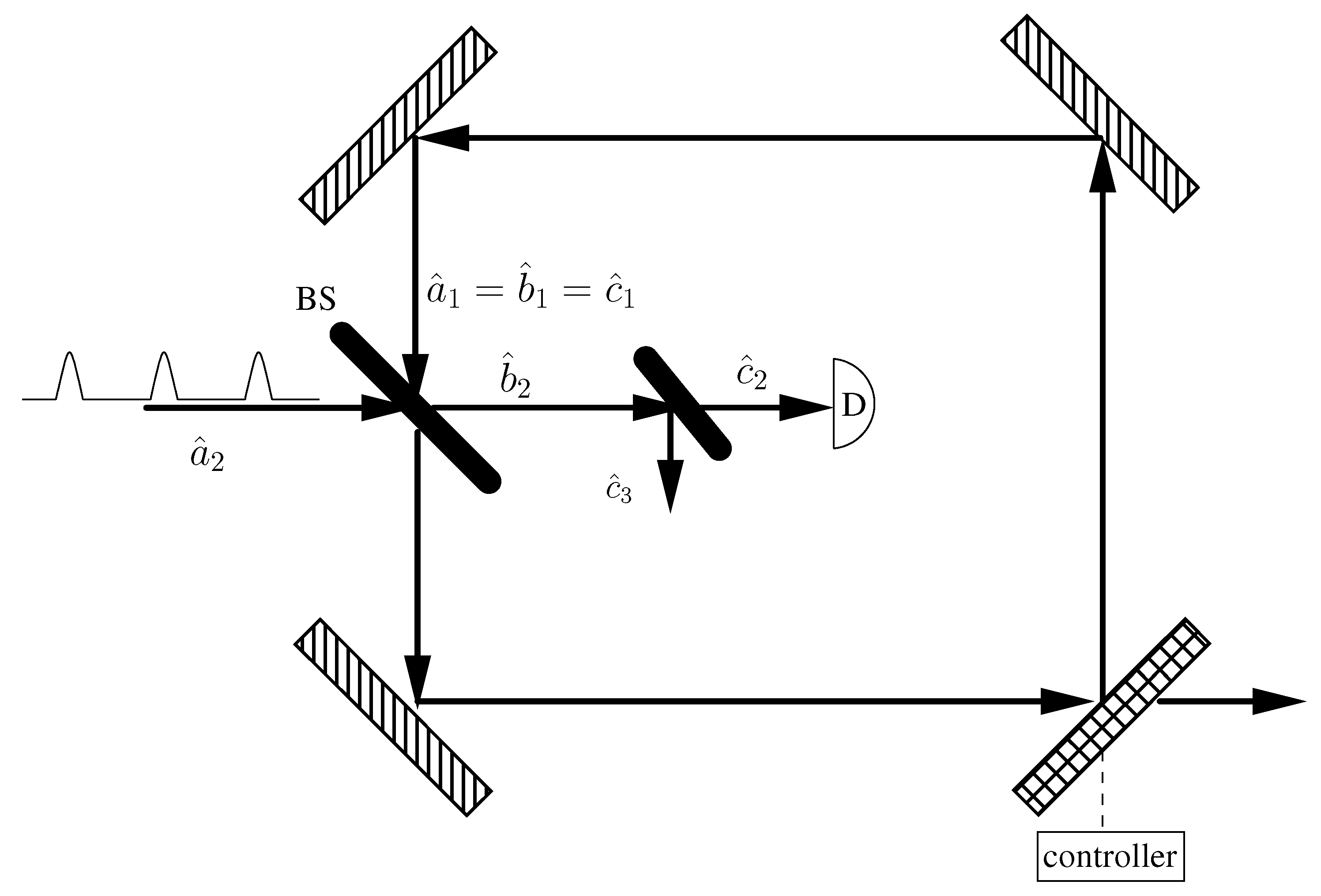
3.1. Photon Addition with a Beam Splitter and a Detector

Our loop scheme can be replaced by a periodic system consisting of beam splitters and ideal detectors. This can be seen in Figure 2. In one period, there is the main beam splitter with $\tau$ transmittance and the real detector modelled as described previously (with another beam splitter and an ideal detector). At each step, input mode 1 is the same as the output mode except for the first round when it is exactly the vacuum state. Input mode 2 is where the periodic one-photon states come in. Output mode 2 leads to the $\eta$ transmittance beam splitter (i.e., the real detector with $\eta$ efficiency), so it is an input mode of it. Its other input mode is mode 3 where we assume that only vacuum is present, so mode 2 is interfering with the vacuum state at the $\eta$ transmittance beam splitter. From it, the output mode 2 is going towards the ideal detector, and output mode 3 is neglected (i.e., traced out).

Let us look at a general period of this system when n photons are coming to input mode 1 $\left({|n\rangle }_1\right)$, one photon is coming to mode 2 $\left({|1\rangle }_2\right)$, and there is vacuum at mode 3 $\left({|0\rangle }_3\right)$; so, the input photon number state is

$$|{\psi }_{\mathrm{in}}\rangle =|n10\rangle ={\displaystyle \frac{1}{\sqrt{n!}}}{\left(a_1^{†}\right)}^n{a}_2^{†}|000\rangle ,$$

(7)

where, in the last step, we express it with the bosonic creation operators of each input mode acting on the vacuum state.

To obtain the state before the action of the ideal detector, the beam splitter transformations are calculated in the Heisenberg picture: the input creation operators are expressed with the output ones, and this expression is substituted into the creation operator in Equation (7). Switching then to the Schrödinger picture, the output state is obtained by applying this expression of the output creation operator to the vacuum state of the output modes.

First, we examine the effect of the first (main) beam splitter with $\tau$ transmittance. It can be described similarly to what we have already presented in (6), but now, we have a third input mode, which is not affected by this beam splitter, so its effect on the creation operators is the following:

$$\left(\begin{array}{c}{\widehat{a}}_1^{†}\\ {\widehat{a}}_2^{†}\\ {\widehat{a}}_3^{†}\end{array}\right)=\left(\begin{array}{ccc}\sqrt{\tau }& -\sqrt{1-\tau }& 0\\ \sqrt{1-\tau }& \sqrt{\tau }& 0\\ 0& 0& 1\end{array}\right)\left(\begin{array}{c}{\widehat{b}}_1^{†}\\ {\widehat{b}}_2^{†}\\ {\widehat{b}}_3^{†}\end{array}\right).$$

(8)

Using this, the output state of the $\tau$ transmittance beam splitter is

$$\begin{array}{c}|{\psi }_{\mathrm{out}}\rangle ={\displaystyle \frac{1}{\sqrt{n!}}}{\left(\sqrt{\tau }·{\widehat{b}}_1^{†}-\sqrt{1-\tau }·{\widehat{b}}_2^{†}\right)}^n\left(\sqrt{1-\tau }·{\widehat{b}}_1^{†}+\sqrt{\tau }·{\widehat{b}}_2^{†}\right)|000\rangle =\hfill \\ ={(-1)}^n\sqrt{{\displaystyle \frac{\tau {(1-\tau )}^n}{n!}}}{\left({\widehat{b}}_2^{†}\right)}^{n+1}|000\rangle +\\ +\sum _{k=1}^n{(-1)}^{n-k}\sqrt{{\displaystyle \frac{{\tau }^{k-1}{(1-\tau )}^{n-k}}{n!}}}\left[\left({\displaystyle \genfrac{}{}{0pt}{}{n}{k}}\right)\tau -\left({\displaystyle \genfrac{}{}{0pt}{}{n}{k-1}}\right)(1-\tau )\right]{\left({\widehat{b}}_1^{†}\right)}^k{\left({\widehat{b}}_2^{†}\right)}^{n-k+1}|000\rangle +\\ \hfill +\sqrt{{\displaystyle \frac{{\tau }^n(1-\tau )}{n!}}}{\left({\widehat{b}}_1^{†}\right)}^{n+1}|000\rangle ,\end{array}$$

(9)

where the vacuum state on the right-hand side is understood in the modes defined by the $\widehat{b}$ operators; thus, e.g., ${\widehat{b}}_1^{†}|000\rangle =|100\rangle$.

Now, we have to apply the effect of the other beam splitter (standing in front of an ideal detector with $\eta$ transmittance) in this state. It can be expressed similarly:

$$\left(\begin{array}{c}{\widehat{b}}_1^{†}\\ {\widehat{b}}_2^{†}\\ {\widehat{b}}_3^{†}\end{array}\right)=\left(\begin{array}{ccc}1& 0& 0\\ 0& \sqrt{\eta }& \sqrt{1-\eta }\\ 0& -\sqrt{1-\eta }& \sqrt{\eta }\end{array}\right)\left(\begin{array}{c}{\widehat{c}}_1^{†}\\ {\widehat{c}}_2^{†}\\ {\widehat{c}}_3^{†}\end{array}\right),$$

(10)

where we introduced ${\widehat{c}}_i^{†}$ as the creation operator of the ith output mode of this beam splitter. Substituting the form of $\widehat{a}$ operators expressed with the $\widehat{c}$ operators, we obtain the following output state:

$$\begin{array}{c}|{\psi }_{\mathrm{out}}^{\prime }\rangle =\sum _{k=0}^{n+1}{(-1)}^n\sqrt{{\displaystyle \frac{\tau {(1-\tau )}^n}{n!}}}\left({\displaystyle \genfrac{}{}{0pt}{}{n+1}{k}}\right)\sqrt{{\eta }^{n-k+1}{(1-\eta )}^k}{\left({\widehat{c}}_2^{†}\right)}^{n-k+1}{\left({\widehat{c}}_3^{†}\right)}^k|000\rangle +\hfill \\ +\sum _{k=1}^n\sum _{l=0}^{n-k+1}{(-1)}^{n-k}\sqrt{{\displaystyle \frac{{\tau }^{k-1}{(1-\tau )}^{n-k}}{n!}}}\sqrt{{\eta }^{n-k-l+1}{(1-\eta )}^l}\times \\ \times \left[\left({\displaystyle \genfrac{}{}{0pt}{}{n}{k}}\right)\tau -\left({\displaystyle \genfrac{}{}{0pt}{}{n}{k-1}}\right)(1-\tau )\right]\left({\displaystyle \genfrac{}{}{0pt}{}{n-k+1}{l}}\right){\left({\widehat{c}}_1^{†}\right)}^k{\left({\widehat{c}}_2^{†}\right)}^{n-k-l+1}{\left({\widehat{c}}_3^{†}\right)}^l|000\rangle +\\ +\sqrt{{\displaystyle \frac{{\tau }^n(1-\tau )}{n!}}}{\left({\widehat{c}}_1^{†}\right)}^{n+1}|000\rangle =\\ =\sum _{k=0}^{n+1}{(-1)}^n\sqrt{\tau {(1-\tau )}^n{\eta }^{n-k+1}{(1-\eta )}^k}\sqrt{\left({\displaystyle \genfrac{}{}{0pt}{}{n+1}{k}}\right)(n+1)}|0;n-k+1;k\rangle +\\ +\sum _{k=1}^n\sum _{l=0}^{n-k+1}{(-1)}^{n-k}\sqrt{{\tau }^{k-1}{(1-\tau )}^{n-k}{\eta }^{n-k-l+1}{(1-\eta )}^l}\sqrt{\left({\displaystyle \genfrac{}{}{0pt}{}{n-k+1}{l}}\right){\displaystyle \frac{(n-k+1)!k!}{n!}}}\times \\ \times \left[\left({\displaystyle \genfrac{}{}{0pt}{}{n}{k}}\right)\tau -\left({\displaystyle \genfrac{}{}{0pt}{}{n}{k-1}}\right)(1-\tau )\right]|k;n-k-l+1;l\rangle +\\ \hfill +\sqrt{{\tau }^n(1-\tau )}\sqrt{n+1}|n+1;0;0\rangle .\end{array}$$

(11)

Again, the photon number states are now understood in terms of the modes defined by the $\widehat{c}$ operators.

We are interested in the cases when the detector does not detect any photons. This state can be obtained by a projection. The operator we can use for this is

$${\widehat{\mathbb{I}}}^{\left(1\right)}\otimes {\widehat{P}}_0^{\left(2\right)}\otimes {\widehat{\mathbb{I}}}^{\left(3\right)}=\sum _{i=0}^{\infty }{|i\rangle }_1{\langle i|}_1\otimes {|0\rangle }_2{\langle 0|}_2\otimes \sum _{j=0}^{\infty }{|j\rangle }_3{\langle j|}_3,$$

(12)

where ${\mathbb{I}}^{\left(i\right)}$ is the identity of the ith mode and $P_k^{\left(i\right)}={|k\rangle }_i{\langle k|}_i$ is the projector of the ith mode projecting to the k-photon state. Applying this operator on $|{\psi }_{\mathrm{out}}^{\prime }\rangle$, we obtain

$$\begin{array}{c}{\widehat{\mathbb{I}}}^{\left(1\right)}\otimes {\widehat{P}}_0^{\left(2\right)}\otimes {\widehat{\mathbb{I}}}^{\left(3\right)}|{\psi }_{\mathrm{out}}^{\prime }\rangle =\hfill \\ ={(-1)}^n\sqrt{\tau {(1-\tau )}^n{(1-\eta )}^{n+1}}\sqrt{n+1}|0;0;n+1\rangle +\\ +\sum _{k=1}^n{(-1)}^{n-k}\sqrt{{\tau }^{k-1}{(1-\tau )}^{n-k}{(1-\eta )}^{n-k+1}}\sqrt{{\displaystyle \frac{(n-k+1)!k!}{n!}}}\times \\ \hfill \times \left[\left({\displaystyle \genfrac{}{}{0pt}{}{n}{k}}\right)\tau -\left({\displaystyle \genfrac{}{}{0pt}{}{n}{k-1}}\right)(1-\tau )\right]|k;0;n-k+1\rangle +\sqrt{{\tau }^n(1-\tau )}\sqrt{n+1}|n+1;0;0\rangle .\end{array}$$

(13)

Its absolute value squared is the probability of not detecting any photon with the detector. It is

$$p=\left({\eta }^2\tau \left(1-\tau \right)\left(n+1\right)+1-\eta \right){\left(\eta \tau +1-\eta \right)}^{n-1}$$

(14)

that equals to the sum of all possible $|k;0;n-k+1\rangle$ states’ probability, for instance, in the basic Hong–Ou–Mandel setup with $\tau =0.5$ as an example and an ideal detector $\left(\eta =1\right)$. In this case, p decreases exponentially (we note that, usually, apart from some special cases, p decreases exponentially):

$$p(n,\tau =0.5,\eta =1)=\left(n+1\right)2^{-n-1}.$$

(15)

We return back to the general case. After the projection, the state we have obtained is not normalised; that is why we have to multiply it with $1/\sqrt{p}$ to obtain a properly normalised photon state:

$$\begin{array}{c}{|{\psi }_{\mathrm{out},}\mathrm{norm}\rangle }_{13}={\displaystyle \frac{1}{\sqrt{p}}}\{{(-1)}^n\sqrt{\tau {(1-\tau )}^n{(1-\eta )}^{n+1}}\sqrt{n+1}{|0;n+1\rangle }_{13}+\hfill \\ +\sum _{k=1}^n{(-1)}^{n-k}\sqrt{{\tau }^{k-1}{(1-\tau )}^{n-k}{(1-\eta )}^{n-k+1}}\sqrt{{\displaystyle \frac{(n-k+1)!k!}{n!}}}\times \\ \hfill \times \left[\left({\displaystyle \genfrac{}{}{0pt}{}{n}{k}}\right)\tau -\left({\displaystyle \genfrac{}{}{0pt}{}{n}{k-1}}\right)(1-\tau )\right]{|k;n-k+1\rangle }_{13}+\sqrt{{\tau }^n(1-\tau )}\sqrt{n+1}{|n+1;0\rangle }_{13}\}.\end{array}$$

(16)

Here, we no longer denote the photon number in mode 2, because it is 0 in every component. Now, with the two remaining modes 1 and 3, we can obtain the density matrix as follows:

$$\widehat{\rho }={|{\psi }_{\mathrm{out},}\mathrm{norm}\rangle }_{13}{\langle {\psi }_{\mathrm{out},}\mathrm{norm}|}_{13}.$$

(17)

As we described earlier, output mode 3 is ignored, so we have to trace it out:

$$\begin{array}{c}{\widehat{\rho }}_1={Tr}_3\widehat{\rho }={\displaystyle \frac{1}{p}}\left\{\tau {(1-\tau )}^n{(1-\eta )}^{n+1}(n+1){|0\rangle }_1{\langle 0|}_1+\right.\hfill \\ +\sum _{k=1}^n{\tau }^{k-1}{(1-\tau )}^{n-k}{(1-\eta )}^{n-k+1}{\displaystyle \frac{(n-k+1)!k!}{n!}}{\left[\left({\displaystyle \genfrac{}{}{0pt}{}{n}{k}}\right)\tau -\left({\displaystyle \genfrac{}{}{0pt}{}{n}{k-1}}\right)(1-\tau )\right]}^2{|k\rangle }_1{\langle k|}_1+\\ \hfill \left.+{\tau }^n(1-\tau )(n+1){|n+1\rangle }_1{\langle n+1|}_1\right\}.\end{array}$$

(18)

Note that this state is diagonal in the photon number basis; i.e., it is an incoherent mixture of photon number states. This fact will be useful later. The fidelity of the state in Equation (18) can be obtained as the coefficient of the ${|n+1\rangle }_1{\langle n+1|}_1$ term

$$F(n,\tau ,\eta )={\displaystyle \frac{{\tau }^n(1-\tau )(n+1)}{p(n,\tau ,\eta )}}.$$

(19)

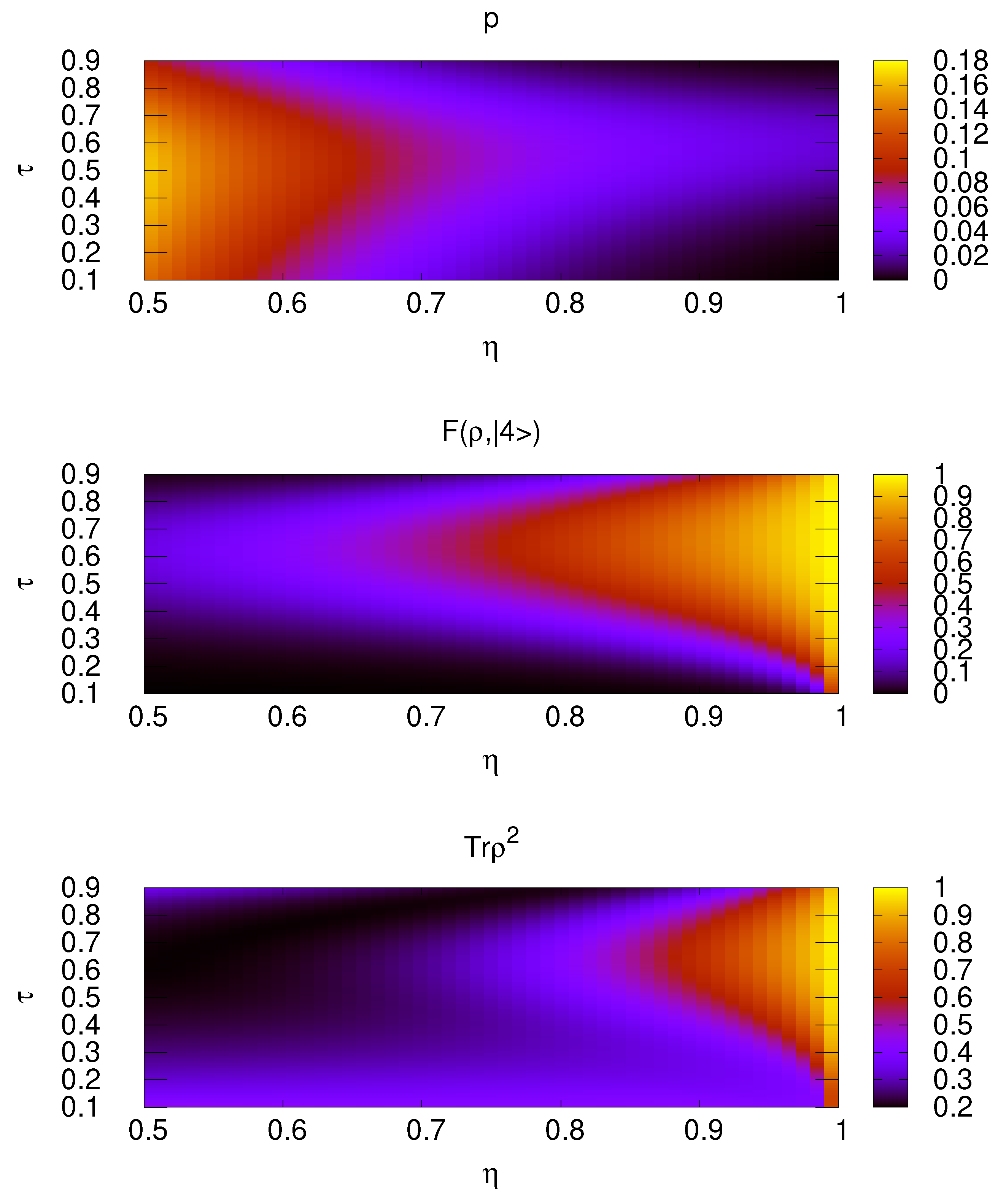
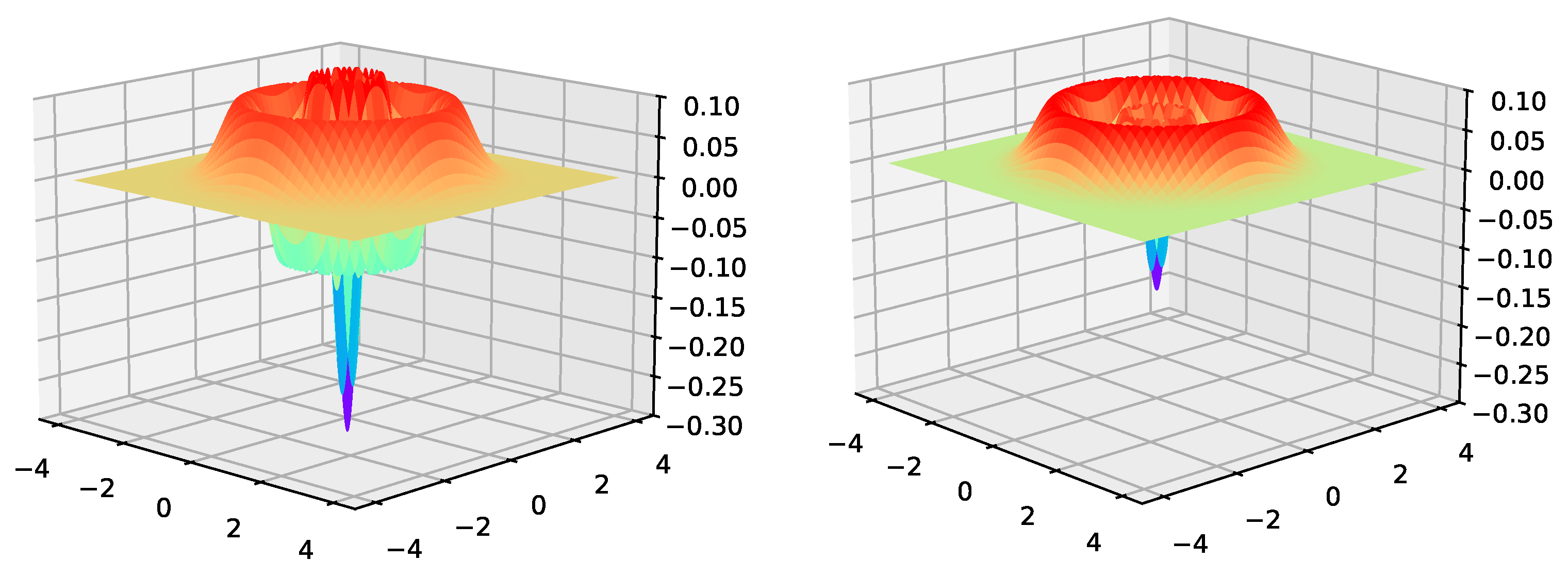
3.2. Iterated Photon Addition

Having discussed the case when a single photon is added to an n-photon state, let us now turn our attention to the case when mode 1 is not in an n-photon state but in the state coming from the previous photon addition. Because of the imperfect detection, it will be a mixture of photon number states.

In particular, consider the case of a train of n single-photon pulses arriving at our arrangement, having a beam splitter of transmittance $\tau$ and a detector of efficiency $\eta$. After the n pulses, the result is coupled out.

As before, let us denote the absorption operators of the modes after an iteration—i.e., at the stage before the next input pulse arrives and when the detection takes place, after the beam splitter modelling detector loss—using ${\widehat{c}}_1$, ${\widehat{c}}_2$, and ${\widehat{c}}_3$, respectively. Before the beam splitter modelling loss, we have the operators $\widehat{b}$ given by Equation (10), which are expressed with the absorption operators $\widehat{a}$ at the arrival of the input pulse of this turn according to Equation (8). As pointed out before (see Equation (18)), on the condition that the detector never fires, at each iteration, the state in mode 1 emerges from the previous iteration, ${\rho }^{(1,n)}$, which is now the input state in mode 2 of the next iteration, and $n+1$ is an incoherent mixture of photon number states up to n photons: ${\rho }^{(1,n)}$ is diagonal in the photon number basis.

This makes it possible to calculate the output at the iteration the output in the following way. We first calculate the state before the projective measurement as if we had exactly k photons at the input mode 2 of the beam splitter at the beginning of the iteration; we perform this for all the k values that occur at this iteration. Hence, k ranges from 1 to n. This conditional state can be calculated as

$$|{\Psi }_{3|k}\rangle ={\displaystyle \frac{1}{\sqrt{k!}}}{\left({\widehat{a}}_1{({\widehat{c}}_1^{†},{\widehat{c}}_2^{†},{\widehat{c}}_3^{†})}^{†}\right)}^k{\widehat{a}}_2{({\widehat{c}}_1^{†},{\widehat{c}}_2^{†},{\widehat{c}}_3^{†})}^{†}|000\rangle ,$$

(20)

where the $\widehat{a}$ operators are expressed with the $\widehat{c}$ operators in order to obtain the state after the beam splitter; see also Equation (11).

As the input at each iteration there is an incoherent mixture of the respective k-photon possibilities coming from the previous iteration, the output can be obtained by mixing the conditional outputs with the respective probabilities ${\varrho }_{k,k}^{(1,n)}$, resulting in the density matrix of the three-mode field before the (ideal) detection:

$${\varrho }^{(n+1,\mathrm{preproj})}=\sum _{k=0}^n{\rho }_{k,k}^{(1,n)}|{\Psi }_{3|k}\rangle \langle {\Psi }_{3|k}|.$$

(21)

The ideal detection is described then with a projection of this three-mode density operator to the vacuum state in mode 2, leading to the unnormalised density operator

$${\varrho }^{(n+1,\mathrm{afterproj})}={|0\rangle }_2{\langle 0|}_2{\varrho }^{(n+1,\mathrm{preproj})}{|0\rangle }_2{\langle 0|}_2.$$

(22)

From this, the probability of the vacuum detection, i.e., that of obtaining an approximate n + 1 photon state on the condition that the previous iteration succeeded is

$$p_{n+1|n}=Tr{\varrho }^{(n+1,\mathrm{afterproj})},$$

(23)

whereas the state of mode 1 after this iteration, which will be the input to the next iteration, or the output if the desired number of iterations has taken place, will read as

$${\rho }^{(1,n+1)}={\displaystyle \frac{1}{p_{n+1|n}}}{Tr}_{2,3}{\varrho }^{(n+1,\mathrm{afterproj})}.$$

(24)

As pointed out before, this will remain diagonal. The net success probability will be the product of success probabilities at each turn,

$$p_{n+1}=\prod _{k=0}^{n+1}{p}_{n+1|n}.$$

(25)

These iterations can be evaluated numerically. We have performed the numerical calculations with version 5.0.4 of the QuTiP Quantum Toolbox in Python [30,31,32], which is capable of performing calculations with multimode quantum states and density operators represented in the photon number basis (truncated at the highest possible photon number in the system). It also implements creation and annihilation operators, partial traces, and projections. Hence, numerically evaluating the described iterations is straightforward.

As examples, we have considered the cases of generating three or four photons in this setup, as they offer reasonable success probabilities and fidelities. In Figure 3 and Figure 4, we have plotted the net success probability, the fidelity of the output state to the desired number state, and the output purity $Tr{\varrho }^2$, for the three- and four-photon cases, respectively, as a function of detector efficiency $\eta$ and beam splitter transmittance $\tau$.

The figures support the following conclusions. Lower detector efficiencies yield to bigger success probabilities; the detector loss results in a more frequent detection of vacuum. Meanwhile, the fidelity and the purity do not decrease too dramatically with the detector efficiency; e.g., in the three-photon case, a detector with an efficiency of $80\%$ will give a fidelity of $0.67$ with a symmetric beam splitter, with a success probability of $0.14$. This is to be compared with the case of the ideal detector where the fidelity is 1 but the success probability is $0.09$.

While the lower fidelity can be a significant issue in certain applications, we remark that such a state is still highly nonclassical: its Wigner function is very similar in shape to that of the $|3\rangle$ state, with a relevant negative part, as illustrated in Figure 5.

Another phenomenon to be observed in the figures is that, for a given detector efficiency, non-symmetric beam splitters may give better performance. This is even more marked in the case of the four-photon state, although the results also confirm that the success probability becomes extremely low as expected.

Finally, let us briefly consider certain other imperfections that can affect our scheme. One of these is the potential appearance of the vacuum or two-photon state in the single-photon pulses. (We consider the probability of three-photon states as negligible.) This situation can be modelled so that instead of the quantum state ${|1\rangle }_2$, the mixture $q_0{|0\rangle }_2{\langle 0|}_2+q_1{|1\rangle }_2{\langle 1|}_2+q_2{|2\rangle }_2{\langle 2|}_2$ arrives in each pulse. Here, $q_1\gg q_0,q_2$, and $q_0+q_1+q_2=1$. It can be easily shown along the same arguments as described before that the density matrix replacing the one in Equation (18) will still be diagonal. This facilitates a similar numerical evaluation of this case. As expected, this imperfection will lead to fidelities lower than those for the ideal case. For instance, in the already-discussed three-photon case with a detector efficiency of $80\%$ which gave a fidelity of $0.67$ and probability of $0.14$ with a symmetric beam splitter, considering $q_0=0.08,q_1=0.9,q_2=0.02$, the fidelity will become $0.44$, with a success probability of $0.16$. The fidelity is thus still reasonable, while the increased probability is due to the increased chance of detecting vacuum because of the possibility of zero photons in the pulses.

Another possible issue could be that of the imperfections in the timing, which may hinder the matching of spatiotemporal modes, that is, the indistinguishability of the interfering photons, thereby decreasing fidelity and success probability of the scheme. This could be due to the jitter in the photon pulse arrival times or stability issues in the arm lengths of the interferometers. In the case of Hong–Ou–Mandel interference, this had already been analysed in the original paper [1], and Ref. [2] provides a very detailed account on the method of detailed calclation. The present scheme could be also analysed along the same lines, but the detailed description is beyond the scope of this manuscript, and it depends on many potential experimental details, such as, e.g., assumptions on pulse shapes. It can be stated though, that just like in the case of Hong–Ou–Mandel interference, mode matching is a necessary condition for the scheme to work. The period time of periodic single-photon sources is determined by the periodicity of their pumping laser, which can be set rather accurately, and accurate locking of the arm lengths has to be maintained.

4. Discussion and Conclusions

We have considered an iterated photon addition scheme using a single detector and a beam splitter, which probabilistically converts a train of single-photon pulses into a higher photon number state. Using non-ideal detectors, the scheme outputs a mixture of photon states which can be still close to the desired n-photon state and exhibits nonclassical properties such as negativity of the Wigner function. Although the success probability of the scheme decreases, exponentially with n, three- or four-photon states can be generated still with reasonable probability. This probability increases when using an non-ideal detector; however, the fidelity of the generated state to the desired Fock-state decreases. We have analysed in detail this interplay between the success probability and the fidelity. We have found that, in certain cases, a better fidelity can be achieved by using a beam splitter with optimally chosen transmittance. The presented scheme thus offers a relatively simple way of generating highly nonclassical states of time-bin modes. A logical continuation of the present research could be the replacement of the beam splitter with a nonlinear element and a detailed comparison with a classical description of the scheme.

Viewed from a broader context, time-multiplexed photon interference schemes are seeing significant development. For instance, in addition to the time-bin, the resolved (local) approach studied here has been extended to time-bucket (global) coincidence, showing nonclassical effects beyond Hong–Ou–Mandel-type interference [33]. In this experimental context, the present schema could easily realised, provided that a periodic single-photon source is available; the latter is also important in photonic quantum information applications. Let us also remark that certain optical quantum processors, such as Borealis, also employ delay loops [34]; hence, the present results can be instructive also for the detailed understanding of these processors.

References

1. Hong, C.K.; Ou, Z.Y.; Mandel, L. Measurement of subpicosecond time intervals between two photons by interference. Phys. Rev. Lett. 1987, 59, 2044–2046. [Google Scholar] [CrossRef] [PubMed]
2. Drago, C.; Brańczyk, A.M. Hong–Ou–Mandel interference: A spectral–temporal analysis. Can. J. Phys. 2024, 102, 411–421. [Google Scholar] [CrossRef]
3. Zavatta, A.; Viciani, S.; Bellini, M. Quantum-to-Classical Transition with Single-Photon-Added Coherent States of Light. Science 2004, 306, 660–662. [Google Scholar] [CrossRef] [PubMed]
4. Zavatta, A.; Viciani, S.; Bellini, M. Single-photon excitation of a coherent state: Catching the elementary step of stimulated light emission. Phys. Rev. A 2005, 72, 23820. [Google Scholar] [CrossRef]
5. Zavatta, A.; Parigi, V.; Bellini, M. Experimental nonclassicality of single-photon-added thermal light states. Phys. Rev. A 2007, 75, 052106. [Google Scholar] [CrossRef]
6. Parigi, V.; Zavatta, A.; Kim, M.; Bellini, M. Probing Quantum Commutation Rules by Addition and Subtraction of Single Photons to/from a Light Field. Science 2007, 317, 1890–1893. [Google Scholar] [CrossRef]
7. Akhtar, N.; Wu, J.; Peng, J.X.; Liu, W.M.; Gao, X. Sub-Planck structures and sensitivity of the superposed photon-added or photon-subtracted squeezed-vacuum states. Phys. Rev. A 2023, 107, 052614. [Google Scholar] [CrossRef]
8. Biagi, N.; Francesconi, S.; Zavatta, A.; Bellini, M. Photon-by-photon quantum light state engineering. Prog. Quantum Electron. 2022, 84, 100414. [Google Scholar] [CrossRef]
9. Holmes, C.A.; Milburn, G.J.; Walls, D.F. Photon-number-state preparation in nondegenerate parametric amplification. Phys. Rev. A 1989, 39, 2493–2501. [Google Scholar] [CrossRef]
10. Dotsenko, I.; Mirrahimi, M.; Brune, M.; Haroche, S.; Raimond, J.M.; Rouchon, P. Quantum feedback by discrete quantum nondemolition measurements: Towards on-demand generation of photon-number states. Phys. Rev. A 2009, 80, 013805. [Google Scholar] [CrossRef]
11. Varcoe, B.T.H.; Brattke, S.; Weidinger, M.; Walther, H. Preparing pure photon number states of the radiation field. Nature 2000, 403, 743–746. [Google Scholar] [CrossRef] [PubMed]
12. Brattke, S.; Varcoe, B.T.H.; Walther, H. Generation of Photon Number States on Demand via Cavity Quantum Electrodynamics. Phys. Rev. Lett. 2001, 86, 3534–3537. [Google Scholar] [CrossRef] [PubMed]
13. Sayrin, C.; Dotsenko, I.; Zhou, X.; Peaudecerf, B.; Rybarczyk, T.; Gleyzes, S.; Rouchon, P.; Mirrahimi, M.; Amini, H.; Brune, M.; et al. Real-time quantum feedback prepares and stabilizes photon number states. Nature 2011, 477, 73–77. [Google Scholar] [CrossRef] [PubMed]
14. Brattke, S.; Guthöhrlein, G.R.; Keller, M.; Lange, W.; Varcoe, B.; Walther, H. Generation of photon number states on demand. J. Mod. Opt. 2003, 50, 1103–1113. [Google Scholar] [CrossRef]
15. Hofheinz, M.; Weig, E.M.; Ansmann, M.; Bialczak, R.C.; Lucero, E.; Neeley, M.; O’Connell, A.D.; Wang, H.; Martinis, J.M.; Cleland, A.N. Generation of Fock states in a superconducting quantum circuit. Nature 2008, 454, 310–314. [Google Scholar] [CrossRef]
16. Cosacchi, M.; Wiercinski, J.; Seidelmann, T.; Cygorek, M.; Vagov, A.; Reiter, D.E.; Axt, V.M. On-demand generation of higher-order Fock states in quantum-dot–cavity systems. Phys. Rev. Res. 2020, 2, 033489. [Google Scholar] [CrossRef]
17. Waks, E.; Diamanti, E.; Yamamoto, Y. Generation of photon number states. New J. Phys. 2006, 8, 4. [Google Scholar] [CrossRef]
18. Cooper, M.; Wright, L.J.; Söller, C.; Smith, B.J. Experimental generation of multi-photon Fock states. Opt. Express 2013, 21, 5309–5317. [Google Scholar] [CrossRef]
19. Sonoyama, T.; Takahashi, K.; Sano, T.; Suzuki, T.; Nomura, T.; Yabuno, M.; Miki, S.; Terai, H.; Takase, K.; Asavanant, W.; et al. Generation of multi-photon Fock states at telecommunication wavelength using picosecond pulsed light. Opt. Express 2024, 32, 32387–32395. [Google Scholar] [CrossRef]
20. Zhang, S.; Dong, Y.; Zou, X.; Shi, B.; Guo, G. Continuous-variable-entanglement distillation with photon addition. Phys. Rev. A 2013, 88, 32324. [Google Scholar] [CrossRef]
21. Bodog, F.; Mechler, M.; Koniorczyk, M.; Adam, P. Optimization of multiplexed single-photon sources operated with photon-number-resolving detectors. Phys. Rev. A 2020, 102, 013513. [Google Scholar] [CrossRef]
22. Meyer-Scott, E.; Silberhorn, C.; Migdall, A. Single-photon sources: Approaching the ideal through multiplexing. Rev. Sci. Instrum. 2020, 91, 3320. [Google Scholar] [CrossRef] [PubMed]
23. Arakawa, Y.; Holmes, M.J. Progress in quantum-dot single photon sources for quantum information technologies: A broad spectrum overview. Appl. Phys. Rev. 2020, 7, 021309. [Google Scholar] [CrossRef]
24. Adam, P.; Mechler, M. Single-photon sources based on incomplete binary-tree multiplexers with optimal structure. Opt. Express 2023, 31, 30194–30211. [Google Scholar] [CrossRef]
25. Li, R.; Liu, F.; Lu, Q. Quantum Light Source Based on Semiconductor Quantum Dots: A Review. Photonics 2023, 10, 639. [Google Scholar] [CrossRef]
26. Adam, P.; Mechler, M. Single-photon sources based on stepwise optimized binary-tree multiplexers. Opt. Express 2024, 32, 17173–17188. [Google Scholar] [CrossRef]
27. Campos, R.A.; Saleh, B.E.; Teich, M.C. Quantum-mechanical lossless beam splitter: SU (2) symmetry and photon statistics. Phys. Rev. A 1989, 40, 1371. [Google Scholar] [CrossRef]
28. Schreiber, A.; Cassemiro, K.N.; Potoček, V.; Gábris, A.; Mosley, P.J.; Andersson, E.; Jex, I.; Silberhorn, C. Photons Walking the Line: A Quantum Walk with Adjustable Coin Operations. Phys. Rev. Lett. 2010, 104, 050502. [Google Scholar] [CrossRef]
29. Lubasch, M.; Valido, A.A.; Renema, J.J.; Kolthammer, W.S.; Jaksch, D.; Kim, M.S.; Walmsley, I.; García-Patrón, R. Tensor network states in time-bin quantum optics. Phys. Rev. A 2018, 97, 062304. [Google Scholar] [CrossRef]
30. QuTiP Quantum Toolbox in Python. 2012. Available online: https://qutip.org (accessed on 5 November 2024).
31. Johansson, J.; Nation, P.; Nori, F. QuTiP: An open-source Python framework for the dynamics of open quantum systems. Comput. Phys. Commun. 2012, 183, 1760–1772. [Google Scholar] [CrossRef]
32. Johansson, J.; Nation, P.; Nori, F. QuTiP 2: A Python framework for the dynamics of open quantum systems. Comput. Phys. Commun. 2013, 184, 1234–1240. [Google Scholar] [CrossRef]
33. Nitsche, T.; De, S.; Barkhofen, S.; Meyer-Scott, E.; Tiedau, J.; Sperling, J.; Gábris, A.; Jex, I.; Silberhorn, C. Local Versus Global Two-Photon Interference in Quantum Networks. Phys. Rev. Lett. 2020, 125, 213604. [Google Scholar] [CrossRef] [PubMed]
34. Madsen, L.S.; Laudenbach, F.; Askarani, M.F.; Rortais, F.; Vincent, T.; Bulmer, J.F.F.; Miatto, F.M.; Neuhaus, L.; Helt, L.G.; Collins, M.J.; et al. Quantum computational advantage with a programmable photonic processor. Nature 2022, 606, 75–81. [Google Scholar] [CrossRef]
Figure 1. The scheme considered in the present manuscript: a train of single-photon pulses enters the system in mode 2. The system consists of an interference loop. Mode 2 is subjected to a projective measurement to the vacuum state. Detector loss is taken into account by the beam splitter in front of the ideal detector D. After the desired number of pulses, the state in mode 1 coupled out by the controller sets the reflectance of the controllable mirror from 1 to 0. If the detector does not fire during the operation, the resulting state is accepted. Otherwise, the operation is unsuccessful, the resulting state has to be disregarded, and the procedure can be repeated. The notation for the annihilation operators is indicated. Note that the scheme is equivalent to the one in Figure 2 in which the quantum states in the modes are explained.
Photonics 11 01075 g001
Figure 2. A periodic system of beam splitters with τ transmittance and real detectors with η efficiency. This is equivalent to the loop scheme presented in Figure 1.
Photonics 11 01075 g002
Figure 3. Success probability (top), output state fidelity (middle), and output state purity (bottom) as a function of detector efficiency η and beam splitter transmittance τ for generating a state approximating | 3 with iterated photon addition.
Photonics 11 01075 g003
Figure 4. Success probability (top), output state fidelity (middle), and output state purity (bottom) as a function of detector efficiency η and beam splitter transmittance τ for generating a state approximating | 4 with iterated photon addition. Observe the negative part of the latter.
Photonics 11 01075 g004
Figure 5. Wigner function of the three-photon Fock-state (left) and that of the approximate three-photon state generated with iterated photon addition with a symmetric beam splitter and a detector with 80 % efficiency resulting from the numerical evaluation (right). The Wigner functions have been calculated from the density operators using the QuTiP package for Python. The coloring of the surface is illustrative, the color schemes of the two subfigures are different.
Photonics 11 01075 g005
Disclaimer/Publisher’s Note: The statements, opinions and data contained in all publications are solely those of the individual author(s) and contributor(s) and not of MDPI and/or the editor(s). MDPI and/or the editor(s) disclaim responsibility for any injury to people or property resulting from any ideas, methods, instructions or products referred to in the content.