The Impact of Afterpulsing Effects in Single-Photon Detectors on the Performance Metrics of Single-Photon Detection Systems

Abstract

A single-photon detection system based on InGaAs SPADs is a high-precision optical measurement system capable of detecting quantum-level optical signals. However, the afterpulsing effect when using InGaAs SPADs severely limits their practical utility. The impact of afterpulsing effects on the performance of systems based on this type of detector can no longer be ignored. Therefore, this paper provides a detailed analysis of the measurement errors induced by afterpulsing effects and proposes a correction method based on a power-law model. This method analyzes the probability distribution of afterpulsing effects using the power-law model and improves the expressions for the system’s average count rate and signal-to-noise ratio by calculating the average number of afterpulses within the average response time. The influence of afterpulse probability and dead time on the system’s average count rate is also analyzed. This afterpulse correction method mitigates the measurement errors caused by afterpulsing effects, thereby enhancing the system’s measurement accuracy.

1. Introduction

Single-photon avalanche diodes (SPADs) are essential devices for low-light detection and have been widely utilized in various fields such as quantum communication [1], LiDAR [2], and remote sensing [3]. Compared to visible light detection, extending the spectral range of SPADs to the shortwave infrared (SWIR) region, particularly at 1550 nm, offers several competitive advantages. These include improved compatibility with the low-loss communication window of optical fibers, increased eye safety thresholds, reduced background solar radiation levels, and enhanced atmospheric transmission through obstructions like smoke and fog [4]. These advantages significantly enhance the efficiency, safety, and application scope of SPADs.

Although silicon-based SPADs have demonstrated excellent performance in the visible to near-infrared range, their application in the SWIR region is limited by the spectral response boundary of silicon material. Vines et al. [4] are working on extending the spectral response range of silicon-based SPADs to the SWIR region by utilizing an innovative planar design for a Ge-on-Si SPAD, which has shown high single-photon detection efficiency and low noise in the SWIR region. Huang et al. [5,6,7] utilized frequency upconversion technology to transfer mid-infrared signals to the response band of silicon-based detectors, thereby achieving both high detection efficiency and low afterpulse probability, though this also increases system complexity. In addition, some progress has also been made in the spectral detection of infrared signals with silicon-based detectors [8,9].

In the SWIR range, the most widely used single-photon detectors are InGaAs/InP SPADs and superconducting nanowire single-photon detectors (SNSPDs) [10,11]. Generally, SNSPDs are favored for their outstanding single-photon detection capability and low afterpulse probability; however, their operation requires cryogenic temperatures below 3K, which limits their widespread use in certain critical applications. In contrast, InGaAs/InP SPADs offer significant advantages in terms of detection wavelength range, operating temperature, and flexibility in system integration, making them the preferred detectors for many advanced photonic applications.

Despite the significant advantages of InGaAs SPADs in the aforementioned aspects, their performance in terms of afterpulsing effects is inferior to that of Si SPADs and SNSPDs. Afterpulsing is caused by the trapping of charges during the avalanche process and their subsequent release, leading to spurious signal counts. This effect severely limits the practicality of InGaAs SPADs, as it reduces the detector’s signal count rate and increases the error rate [12].

Significant progress has been made by various researchers in mitigating afterpulsing effects through different approaches. For example, Tosi et al. [13] developed advanced front-end electronics and fast quenching techniques to reduce afterpulsing. They achieved gated operation at a repetition rate of up to 133 MHz, significantly increasing the count rate while reducing the total charge flow through rapid quenching, effectively lowering the afterpulse probability. Ruggeri et al. [14] introduced a novel integrated circuit that significantly reduces afterpulsing effects in InGaAs/InP SPADs by employing a fast quenching mechanism. This design utilizes sub-nanosecond response times and efficient charge flow control, greatly reducing the occurrence of afterpulsing and thereby enhancing the detector’s performance and count rate, providing robust technical support for high-precision photon detection. Liu et al. [15] effectively suppressed higher-order afterpulsing effects in InGaAs/InP SPADs by introducing a hybrid quenching technique that cleverly combines fast active quenching with high-frequency passive gated quenching. This method significantly reduces the frequency of afterpulsing without sacrificing detection efficiency and improves the performance and reliability of the single-photon detector in free-running mode by physically blocking potential afterpulse release within consecutive gated cycles. Additionally, Ke et al. [16] explored the reduction of afterpulsing by optimizing semiconductor layer structures and improving material quality to decrease charge traps. These studies primarily focus on reducing afterpulsing effects through hardware design improvements and operational strategies. In theoretical research, Ripamonti et al. developed a correction formula for afterpulsing effects in idealized zero dead-time detectors [17], followed by M. Höbel et al. introducing an efficient correction formula for the combined effects of detector dead time and afterpulsing, which is applicable to any kind of detector in multiphoton timing experiments [18].

This paper presents a theoretical study of afterpulsing effects and proposes a correction method based on a power-law model. This method analyzes the probability distribution of afterpulsing effects using the power-law model and refines the expressions for the detector’s average count rate and signal-to-noise ratio by calculating the average afterpulse rate within the average response time. The impact of afterpulse probability and dead time on the average count rate is also analyzed. This correction method effectively mitigates the measurement errors caused by afterpulsing effects, thereby enhancing the measurement accuracy of the system.

2. GM-APD Model and Afterpulsing Model

2.1. GM-APD Model

For SPADs, the detection process follows a Poisson distribution when the count rate is low. Background light and dark counts form the noise sources for the SPADs, which also adhere to the Poisson distribution [19]. Since the sum of Poisson random variables is another Poisson variable, all noise sources are modeled as independent Poisson processes [19,20]. To analyze the entire system’s performance, it is crucial to understand the statistical model of signal and noise arrival times at the detection end. A common single-photon detection model is the GM-APD model [21], as shown in Figure 1.

The SPAD model comprises the photoelectron conversion process and the avalanche multiplication process. The number of signal photons ${\overline{n}}_s$ and background photons ${\overline{n}}_b$ received within a sampling interval is converted into a pre-amplified signal ${\overline{m}}_s$ and background noise signals ${\overline{m}}_b$ through the photoelectron conversion process. Combined with self-generated dark counts ${\overline{m}}_d$ and afterpulse counts ${\overline{m}}_a$, they form the total count $\overline{m}$ before the avalanche multiplication process. The final avalanche signal is obtained after the avalanche multiplication process.

The combined average power of signal and noise, $P$, is the sum of the powers from all components, given as:

$$P=P_s+P_c+P_t+P_d,$$

(1)

where $P_s$, $P_c$, $P_t$, and $P_d$ represent the average signal light power, clutter light power, equivalent average light power produced by thermal noise, and dark current, respectively. In theoretical analysis and system design, considering dark counts as the only source of noise facilitates the simplification of calculations and model construction, thereby making the analytical process more intuitive and comprehensible. Therefore, we utilize the detector’s dark counts to represent the noise component $P_n$ in this study:

$$P=P_s+P_n.$$

(2)

The analysis of performance in traditional methods typically begins with the internal parameters of the detector. In this case, we will analyze performance by converting detection efficiency to external parameters. The detector’s efficiency $\eta$ is ascertainable through computation:

$$\eta ={\displaystyle \frac{1}{\mu }}\ln ({\displaystyle \frac{1-{\tau }_w{C}_{dc}}{1-\raisebox{1ex}{$C_{ph}$}\!\left/ \!\raisebox{-1ex}{$f_L$}\right.}}),$$

(3)

where $\mu$ is the average number of photons contained in each incident light pulse, ${\tau }_w$ is the time window width for counting photons, $C_{dc}$ is the dark counting rate, $C_{ph}$ is the photon count rate, and $f_L$ is the repetition frequency of the laser pulse. The signal counting rate $C_{sig}$ can be obtained by subtracting the dark counting rate $C_{dc}$ from the total photon counting rate $C_{ph}$, as follows:

$$C_{sig}=C-C_{dc}.$$

(4)

2.2. Afterpulsing Model

Afterpulsing results from trapped carriers within the material defects of the SPAD being captured and subsequently released. Previous studies have fitted the observed afterpulsing behavior to various models, among which the multiple exponential model [22,23], the power-law model [24], and the hyperbolic Sinc model [25] are considered more suitable. Ziarkash et al., through the study of afterpulsing behavior and model fitting for different types of detectors, found that the power-law model generally provides the best consistency in terms of results [26]. The expression for the power-law model is as follows:

$$P_a(t)=A·t^{-\lambda },$$

(5)

where $\lambda =1.2\pm 0.2$ represents the effective decay constant, and $A$ is the initial afterpulse probability, which varies with each InGaAs SPAD.

Under ideal conditions, substituting $A=1\%/5\%/10\%/15\%$ and $\lambda =1.2$ into the model and conducting simulations yield the probability curve for afterpulsing, as shown in Figure 2. The larger the value of $A$, the higher the afterpulse probability at any given time point on the curve.

In discussions concerning the afterpulsing phenomena within SPADs, it is crucial to acknowledge the dynamic changes in afterpulse probability. Following each avalanche event, the afterpulse probability decreases over time according to a power-law mode. This decline reflects the gradual release of carriers from their trapped states within the device. We believe that a reset phenomenon typically occurs upon the occurrence of a subsequent avalanche event, as depicted in Figure 3. This reset is caused by the introduction of fresh carriers to the defects by the new avalanche, thereby restarting the computation and decay process of the afterpulse probability. This reset mechanism provides a critical framework for our subsequent calculations of the average afterpulse counts. In the figure, the solid line represents the variation in afterpulse probability following each avalanche, while the dashed line indicates the preparation for the next avalanche, where the afterpulse probability resets.

During detection, each avalanche event in the detector contributes to the afterpulse counts. Therefore, we propose characterizing the afterpulse rate by the number of afterpulses within the average response time.

3. The Average Count Rate and Signal-to-Noise Ratio of the System

In single-photon detection systems, afterpulsing is a common phenomenon that leads to errors in the average count rate and the signal-to-noise ratio (SNR). To optimize system performance, we propose a method based on afterpulsing correction. By accurately calculating the average count of afterpulses, we can more precisely correct the average count rate, reducing the errors caused by afterpulsing. This method also aids in more accurately estimating the noise components within the signal, thereby enhancing the accuracy of the SNR.

3.1. Afterpulsing Correction Method

As mentioned earlier, in SPADs, both signal and noise distributions follow a Poisson distribution. However, afterpulsing does not follow a Poisson distribution and cannot simply be combined with signal light and noise for calculation. To address this issue, in the calculation of the average response of the SPAD, we propose calculating the detector’s average response time, which is the average time for avalanche events caused by a signal, noise, and afterpulsing.

The average signal count for the SPAD is $C_{sig}$, and the average noise count is $C_{dc}$. First, we define the average response time $\tau$, and the number of afterpulses detected during this time is the afterpulsing rate $C_a$. The average response time is determined by the total count detected within a specific time, as follows:

$$\tau ={\displaystyle \frac{1}{C_{\mathrm{sig}}+C_{\mathrm{dc}}+C_{\mathrm{a}}}}={\displaystyle \frac{1}{C+C_{\mathrm{a}}}}.$$

(6)

Integrating the power-law model of the afterpulsing effect over time and then dividing the result of the integration by the total duration of the integration gives the average afterpulsing rate per unit of time. According to the definition, the average count of afterpulses can be obtained from $t_1$ to $t_2$, given as:

$$C_a={\displaystyle \frac{1}{t_2-t_1}}{\displaystyle {\int }_{t_1}^{t_2}{P}_{\mathrm{a}}(t)}dt.$$

(7)

In this paper, we define the time for obtaining the average afterpulse rate as the interval from the start of detection (with a minimal time offset) to the start of the next detection, which is the average response time plus the dead time. For the choice of integration time, we set $t_1=\tau$ and $t_2=t_d+2\tau$, ensuring that the integration covers the entire average response period, including the full timespan from the end of the first response to the end of the next complete response period. This interval includes both those afterpulses that may occur during the dead time and those during the detection period, thereby capturing the detector’s afterpulsing behavior more comprehensively. This time interval includes those afterpulses generated during the dead time, as well as those produced during the detection period, and can be given as:

$$C_a={\displaystyle \frac{1}{\tau }}{\displaystyle {\int }_{\tau }^{t_d+2\tau }{P}_{\mathrm{a}}}dt={\displaystyle \frac{A·\left({\left(t_d+2\tau \right)}^{-\lambda +1}-{\tau }^{-\lambda +1}\right)}{\tau ·\left(-\lambda +1\right)}},$$

(8)

By combining Equations (6) and (8), the relationship between $\tau$ and $C_a$ can be established. The integration operation in the power-law model can be viewed as an accumulated statistic of afterpulse event frequencies over different time intervals. Therefore, it is not merely an estimate of individual afterpulse events but also indirectly includes the interactions between afterpulse events, such as secondary afterpulsing.

3.2. Average Count Rate: Before and After Correction

Without considering afterpulsing effects, the system’s average count rate can be calculated using the following equation, where the average arrival time accounts for the impact of dead time, given as:

$${\xi }_0={\displaystyle \frac{\eta {\overline{n}}_{total}}{1+\eta {\overline{n}}_{total}·t_d}}.$$

(9)

$${\overline{n}}_{total}={\overline{n}}_{\mathrm{s}}+{\overline{n}}_{\mathrm{dc}}=n_{\mathrm{s}}+{\displaystyle \frac{C_{\mathrm{dc}}}{\eta }}$$

(10)

where ${\overline{n}}_{total}$ represents the equivalent number of input photons, ${\overline{n}}_{\mathrm{s}}$ represents the number of signal photons, and ${\overline{n}}_{\mathrm{dc}}$ represents the equivalent dark counts.

After accounting for the afterpulsing effects, the corrected expression for the system’s average count rate can be represented as:

$$\xi ={\displaystyle \frac{\eta n_{total}^{\prime }}{1+\eta n_{total}^{\prime }·t_d}}$$

(11)

$${\overline{n}}_{total}^{\prime }={\overline{n}}_s+{\overline{n}}_{dc}+{\overline{n}}_a={\overline{n}}_s+{\displaystyle \frac{C_{\mathrm{dc}}}{\eta }}+{\displaystyle \frac{C_a}{\eta }}$$

(12)

where ${\overline{n}}_a$ represents the equivalent number of afterpulses.

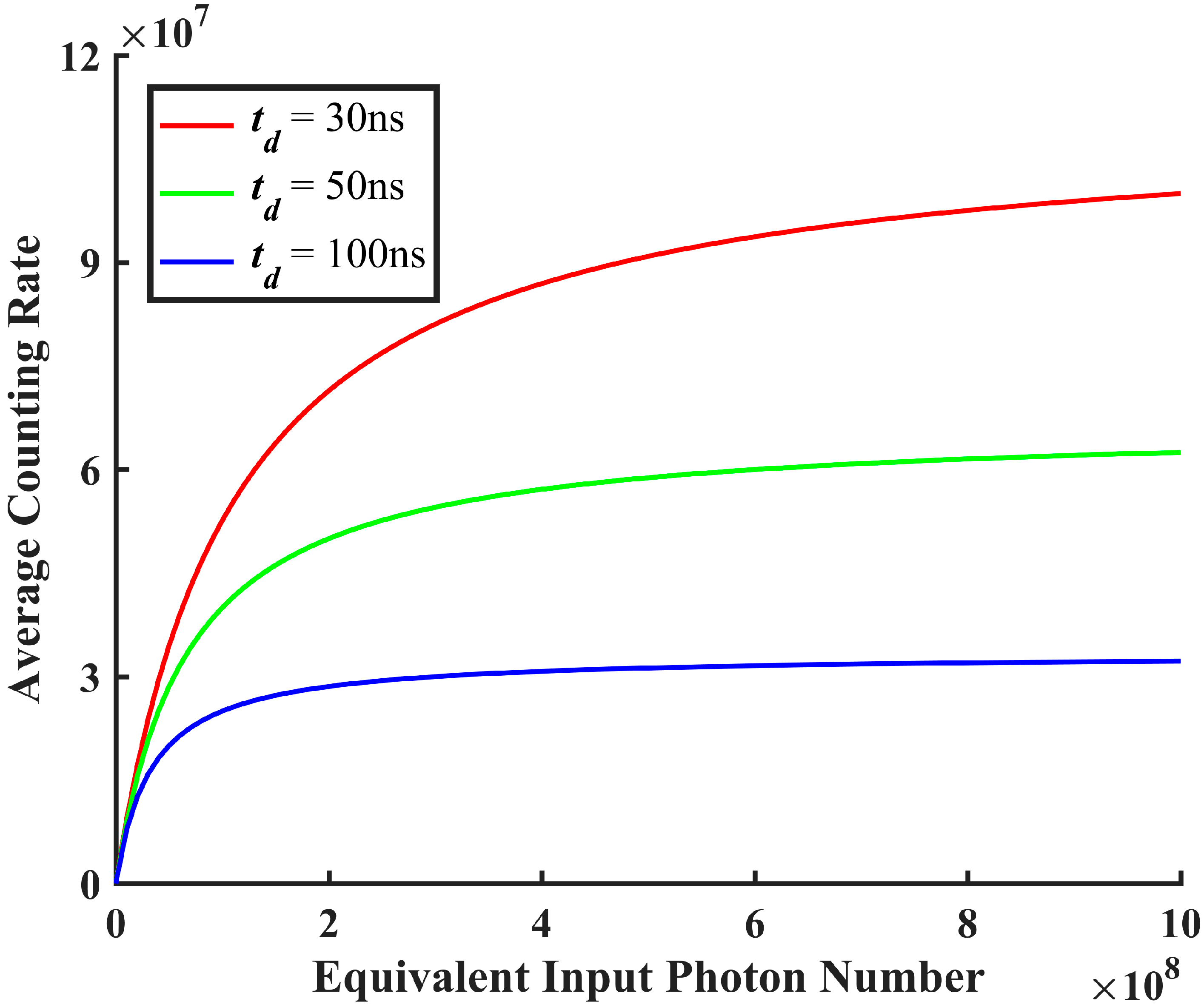
At a detection efficiency of 30% and an initial afterpulse probability of $A=0\%$, the variation curve of the average count rate along with photon number under different dead times is shown in Figure 4. Due to the presence of dead time, there is a theoretical maximum count-rate limit for the detector. This maximum count rate is determined by the reciprocal of the dead time, i.e., maximum count rate = $1/t_d$. The longer the dead time, the lower the average count rate. In reality, due to other factors such as detector recovery time and dark counts, the maximum achievable count rate will always be lower than this theoretical value.

3.3. Signal-to-Noise Ratio: Before and After Correction

Without considering afterpulsing, the SNR for a SPAD based on N-pulse accumulation is defined as the ratio of the square of the detected signal count to the variance of the total detected noise and signal counts [27]. In this paper, $E[M_s]$ and $E[M_n]$ are defined as the total number of signal and noise photons detected upon N-pulse accumulation, respectively, as shown in Equation (14):

$$SNR={\displaystyle \frac{E{[M_s]}^2}{\mathrm{var}[M_s+M]n}},$$

(13)

where $E[M_s]=N{\overline{m}}_s$, $E[M_n]=N{\overline{m}}_n$, and $N$ is the number of pulse accumulations.

In the case where both the GM-APD input and output fluxes follow a Poisson distribution, the mean and variance of the photon number are equal, and we obtain an expression for the signal-to-noise ratio with respect to the incident photon number, given as:

$$SN{R}_o=\eta {\displaystyle \frac{N\times {{\overline{\mathrm{n}}}_s}^2}{{\overline{\mathrm{n}}}_s+{\overline{\mathrm{n}}}_n}}.$$

(14)

Within a set unit of time, the number of input photons and noise photons can be converted into the signal count rate and the dark count rate, respectively, which results in $C_{sig}=\eta {\overline{n}}_s$ and $C_{dc}=\eta {\overline{n}}_n$. Thus, we achieve the following:

$$SN{R}_{\mathrm{o}}={\displaystyle \frac{N\times {C_{sig}}^2}{C_{sig}+C_{dc}}}.$$

(15)

When afterpulsing cannot be ignored, the SNR needs to be recalculated. Afterpulsing can be considered a part of the noise. With the average afterpulsing rate being calculated earlier, it can be incorporated into the SNR expressions in Equations (17) and (18). The equation for SNR then becomes:

$$SNR={\displaystyle \frac{N\times {C_{sig}}^2}{C_{total}}},$$

(16)

where $C_{total}=C_{sig}+C_{dc}+C_a$ and ${\overline{n}}_{total}=\eta C_{total}$, thus:

$$SNR=\eta {\displaystyle \frac{N\times {n_s}^2}{{\overline{\mathrm{n}}}_{total}}}.$$

(17)

4. Systematic Error Analysis and Optimization of Measured Photon Counts

In single-photon detection systems, dead time and afterpulse probability are two crucial parameters that significantly affect the accuracy of the system’s average count rate. To accurately analyze these errors, we need to consider several combinations of different dead times and afterpulse probabilities. Through simulation, we can quantify the impact of these parameters on the average count rate and SNR. This enables us to adjust the dead time and afterpulse probability according to actual needs during the design and optimization of single-photon detection systems, minimizing errors and enhancing the accuracy of the average count rate and SNR.

4.1. Average Count Rate Under Different Afterpulse Probability Conditions

The impact of afterpulse probability in SPADs on the system’s average count rate is evident, with the afterpulsing effect inducing errors in the average count rate that escalate in magnitude concomitant with an increase in afterpulse probability, as shown in Figure 5a. Our statistical analysis indicates that under conditions of low incident photon numbers, the impact of afterpulsing on the system’s average count rate is significant, potentially exceeding 50%. As shown in Figure 5b, with a detector dead time of 50 ns and a detection efficiency of 30%, the error range in the system is between 1.6% and 5.1% when the afterpulse probability is 5% and the incident photon number is high. When the afterpulse probability increases to 10%, the system’s error range expands to between 2.5% and 7.5%.

In SPADs, an elevated afterpulsing probability correlates with an increase in the count errors induced by afterpulsing effects, thereby exacerbating the measurement inaccuracies across the entire system. At lower average photon numbers, the proportion of afterpulsing events within the total count is more significant, due to the relatively fewer real photon detection events, rendering the impact of afterpulsing effects on the average count rate more pronounced. As the number of photons escalates, the relative proportion of afterpulsing events within the total count diminishes, leading to a gradual reduction in the influence of afterpulsing effects on the average count rate.

4.2. Average Count Rate Under Different Dead Times Conditions

Regarding the average count rate of the system, both dead time and afterpulsing exert significant influences. Extended dead times result in a notable reduction in the average count rate and also diminish the contribution of afterpulsing counts to the total count, thereby rendering the measured count rate more closely aligned with the true primary pulse count rate. As shown in Figure 6a, the error induced in the system’s count by afterpulsing effects diminishes with an increase in the detector’s dead time.

As shown in Figure 6b, with the detector’s detection efficiency at 30% and an afterpulse probability of 5%, our data analysis indicates that the system’s error rates are 1.6–5.1% and 0.5–2.0% for dead times of 50 ns and 100 ns, respectively. The influence of afterpulsing effects on the system’s average count rate diminishes with the extension of dead time, as a longer dead time reduces the likelihood of afterpulsing events being erroneously recorded as valid counts. This observation is in alignment with objective reality, further substantiating the reliability of afterpulsing correction measures.

4.3. Signal-to-Noise Ratio Under Different Afterpulse Probabilities

In this section, we assume that $N=100$ and $C_{dc}=1000$, and subsequently calculate the system’s signal-to-noise ratio (SNR) under conditions of 50 ns of dead time with no afterpulsing, and afterpulsing probabilities of 5% and 10%. The variation of the system’s SNR with the number of input photons is illustrated in Figure 7. Considering the additional counts introduced by afterpulsing, there is an increase in the total system noise, resulting in a lower SNR compared to scenarios where afterpulsing is not accounted for.

Data analysis reveals that in scenarios both with and without afterpulsing, the system’s error could reach up to approximately 8%. Incorporating afterpulsing parameters into the SNR calculation implies the consideration of these additional noise sources in the overall noise level. Due to the increased total noise level, the SNR decreases correspondingly, even if the signal level remains constant. An 8% reduction in SNR indicates a relatively significant adverse impact of afterpulsing on system performance, especially in the design and analysis of high-performance optical communication systems or precision measurement systems.

4.4. Optimization of the Measured Photon Count, Based on Afterpulsing Correction

In single-photon detection systems, the afterpulsing effect introduces additional counts, thereby causing measurement errors. To correct this error, we can obtain a stable afterpulse rate through iterative calculation and adjust the actual photon counts in conjunction with the dark count rate, thus achieving more accurate signal photon numbers. The expression for the photon count value $N_{sig}$, corrected for afterpulse probability within the total detection time $T$, is as follows:

$$N_{sig}=N_{total}-{\displaystyle \frac{C_{dc}\times T}{\eta }}-{\displaystyle \frac{C_a\times T}{\eta }},$$

(18)

where $N_{total}$ is the total count by the detector within the detection time $T$, including signal photons, dark counts, and afterpulse counts. Given the known number of incident photons and dark counts, a stable average afterpulse rate $C_a$ can be obtained through iterative calculation, allowing further calculation of the signal photon count after removing afterpulses and dark counts.

Under the conditions of a dead time of 50 ns, a detection efficiency of 30%, a constant input photon count of ${10}^8$, and $C_{dc}=1000$, a simulation was conducted to analyze the effect of different initial afterpulse probabilities on the average count rate and SNR. From this simulation, the maximum afterpulse probability that can be optimized by this method was determined. As shown in Figure 8a, we plotted the percentage increase in the average count rate resulting from an increase in the initial afterpulse probability. The simulation results indicate that when the initial afterpulse probability reaches approximately 40%, the growth in the average count rate nearly stops. Similarly, as shown in Figure 8b, we plotted the percentage decrease in the signal-to-noise ratio (SNR) caused by an increase in the initial afterpulse probability. The results show that at an initial afterpulse probability of 40%, the decrease in SNR is already below 0.2%. Based on the above analysis, we conclude that the maximum optimizable afterpulse probability for this method is approximately 40%.

5. Conclusions

Afterpulsing is a significant parameter in the performance of detectors, and it is crucial for the accurate understanding and optimization of system performance. This study investigates the impact of afterpulsing effects on the performance of single-photon detection systems based on InGaAs SPADs. By calculating the average count of afterpulses within the average response time through the afterpulsing model and incorporating it into the system’s average count rate and SNR, we obtained expressions for the average count rate and SNR that include the afterpulsing effects. Theoretically, afterpulsing effects lead to errors in the system’s average count rate and SNR. The larger the afterpulse probability of the detector, the greater the error caused by the afterpulsing effects. Additionally, we provided an expression for obtaining the photon count, corrected for afterpulse probability from the measured data to improve measurement accuracy.

Despite these promising results, our method may encounter certain limitations in practical applications. The dynamic nature of afterpulsing effects and individual differences in device manufacturing could lead to fluctuations in afterpulse probability, affecting model accuracy. Additionally, environmental factors such as temperature and humidity may influence the afterpulsing behavior. For example, high temperatures can alter charge trapping and release dynamics. As the current model assumes stable environmental conditions, its correction effectiveness might diminish under varying conditions. Future work will consider temperature compensation and environmental monitoring to enhance the method’s adaptability.