Sub-Micron Two-Dimensional Displacement Sensor Based on a Multi-Core Fiber

Abstract

A sub-micron two-dimensional displacement sensor based on a segment of multi-core fiber is presented in this paper. Light at the wavelengths of 1520 nm, 1530 nm, and 1540 nm was introduced separately into three cores of a seven-core fiber (SCF). They were independently transmitted in their respective cores, and after being emitted from the other end of the SCF, they were irradiated onto the end-face of a single-mode fiber (SMF). The SMF received light at three different wavelengths, the power of which was related to the relative position between the SCF and the SMF. When the SMF moved within a two-dimensional plane, the direction of displacement could be determined based on the changes in power at different wavelengths. As a benefit of the high sensitivity of the spectrometer, the sensor could detect displacements at the sub-micron level. When the SMF was translated in 200 nm steps over a range from 5.2 μm to 6.2 μm, the sensitivities at the wavelengths of 1520 nm, 1530 nm, and 1540 nm were 0.34 dB/μm, 0.40 dB/μm, and 0.36 dB/μm, respectively. The two-dimensional displacement sensor proposed in this paper offers the advantages of high detection precision, simple structure, and ease of implementation.

1. Introduction

Optical fiber displacement sensors are pivotal for quantifying the position, displacement, or deformation of objects [1]. They are essential in numerous scientific and technological domains, including industrial automation [2], real-time structural health monitoring [3,4], semiconductor manufacturing [5], aerospace [6,7], and many others. Fiber sensors offer several advantages over conventional electrical sensors, such as higher precision, compactness, superior anti-interference capabilities, and rapid response times [8]. Furthermore, as market demands shift toward high-precision and multi-dimensional measurements, traditional one-dimensional sensors are becoming inadequate. This has spurred the development of advanced technologies, including two-dimensional, high-precision displacement sensors, to address these evolving requirements.

To date, a multitude of two-dimensional fiber displacement sensors have been proposed, each operating on distinct principles. These can be broadly classified into three categories: interferometric [9], fiber Bragg grating [10], and intensity-based sensors [11,12]. Interferometric displacement sensors leverage the principle of light interference to measure displacement. They function by dividing a light beam into two separate beams—one acting as a reference and the other as a measurement beam. When the object under test moves, a phase difference arises between these two beams. The displacement is then ascertained by detecting and analyzing this phase shift. In order to obtain two-dimensional displacement information, a modified extrinsic Fabry–Perot interferometer sensor has been proposed [13]. But this type of sensor provides information on in-plane and out-of-plane displacement. Fiber Bragg grating displacement sensors measure displacement by detecting the shift of the Bragg wavelength. To accomplish two-dimensional displacement measurement, it is essential to modify the symmetrical structure of the fiber’s end-face. Techniques such as employing multi-core fibers [14,15], inscribing gratings directly onto the fiber core and inner cladding [16], or onto the partial core of the depressed cladding fiber [17], have been proposed. While these structures are capable of facilitating two-dimensional displacement sensing, the process of engraving gratings on optical fibers demands sophisticated and costly equipment.

Intensity-based displacement sensors, on the other hand, detect displacement by monitoring variations in the optical intensity within the fiber [18,19,20,21]. The displacement of the measured object modifies the transmission path or the amount of light lost within the fiber, leading to alterations in optical intensity that correspond to the displacement. Compared to interferometric and grating sensors, this sensor type has a simpler operating principle and is more straightforward to implement. By employing single-mode fiber (SMF) bundles [19,20] or plastic multi-core fibers [21] as receivers, the direction of displacement can be ascertained from the variations in power across different fiber cores. However, since plastic multi-core optical fibers are of the multimode variety, the speckle pattern in the spot can impact the measurement accuracy.

With the progress in fiber manufacturing technology, multi-core fibers are finding broader applications in fields such as fiber sensing [22], fiber lasers [23], and fiber communication. Unlike plastic fibers, multi-core fibers sustain the quality of single-mode beams. Furthermore, they provide a more compact structure than SMF bundles. This article introduces a novel two-dimensional displacement sensor that employs multi-core optical fibers. Specifically, a segment of the seven-core fiber (SCF) serves as the transmitting medium, allowing for light of different wavelengths to pass through three of its cores. An SMF then acts as the receiving fiber, capturing the light of these three distinct wavelengths. By monitoring the variations in the light power at these three wavelengths, the sensor is capable of accurately determining both the magnitude and direction of displacement.

2. Working Principle of the Two-Dimensional Displacement Sensor

Figure 1a presents the structure of the two-dimensional displacement sensor proposed in this paper. By aligning the center of the SCF with that of the SMF, the two-dimensional displacement sensor is formed. Generally, multi-core fibers are categorized into strongly coupled and weakly coupled types. In strongly coupled optical fibers, light transmitted through each core experiences coupling between the cores. Conversely, in weakly coupled multi-core fibers, light propagates independently within each core, with each core acting as a separate waveguide. A weakly coupled SCF was employed in our experiment. Figure 1b illustrates the cross-section of the SCF, featuring one central core surrounded by six others. The central core was used for alignment with the SMF. Among the surrounding six cores, three cores were utilized to determine the direction of displacement, while the remaining three cores were not used. During operation, three cores of the SCF were fed with light of different wavelengths. This light propagated independently through the SCF and, upon reaching the SMF, collectively illuminated its core. This allowed for the SMF to receive light that encompassed three distinct wavelengths. Initially, the SMF was aligned with the central core of the SCF. Changes in the relative position between the two fibers altered the intensity of the three wavelengths, and by monitoring these intensity variations, the direction of displacement could be ascertained. Figure 1c shows the distribution of light spots on the end-face of the SMF, with spots of different wavelengths all covering the core of the SMF, which thus received light of three wavelengths. When the SMF moved within the horizontal plane, the intensity of the light received at three different wavelengths varied. These variations allowed for the determination of displacement in two-dimensional directions.

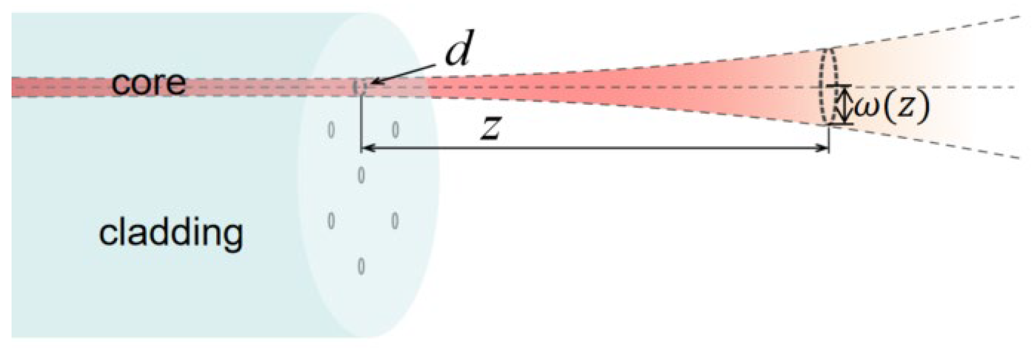
Each core of the SCF can be regarded as an independent waveguide, similar to an SMF. Taking core ① as an example, we analyzed the distribution of light emitted from core ① on the end-face of the SMF. As shown in Figure 2, the light output from the fiber is considered a Gaussian beam, with the beam waist diameter equal to the mode field diameter d of the fiber. By using half of the mode field diameter as the beam waist radius of the Gaussian beam, the spot radius of the beam could be calculated when it reached the SMF.

$$\omega \left(z\right)={\omega }_0\sqrt{1+{\left({\displaystyle \frac{z}{z_R}}\right)}^2}={\displaystyle \frac{d}{2}}\sqrt{1+{\left({\displaystyle \frac{z}{z_R}}\right)}^2},$$

(1)

where ${\omega }_0$ is the waist radius of the Gaussian beam and $\omega \left(z\right)$ is the radius of the light spot when it reaches the end-face of the SMF. z is the distance between the SCF and the SMF, and $z_R$ is the Rayleigh length of the Gaussian beam. The waist radius, ${\omega }_0$, and Rayleigh length of the Gaussian beam satisfy $\pi {\omega }_0^2=\lambda z_R$. d is the mode field diameter of the fiber, which is related to the working wavelength. The irradiance on the end-face of the SMF can be expressed as [24]

$$I\left(r,z\right)={\displaystyle \frac{2P}{\pi {\omega }^2\left(z\right)}}\exp \left[-{\displaystyle \frac{2r^2}{{\omega }^2\left(z\right)}}\right]$$

(2)

In Equation (2), P is the output power of the fiber and r is the distance from the target point to the center of the light spot.

The power of the light at this wavelength received by the SMF is the integral of the irradiance:

$$P\left(z\right)={\displaystyle {\int }_{S}I\left(r,z\right)}dS$$

(3)

In Equation (3), S is the receiving surface, which is the core part of the SMF end-face.

From Equation (3), it can be seen that the optical power received by the SMF is related to the distance, z, and the relative position between the SMF and core, ①. If light with wavelengths is injected into core ①, core ⑤, and core ⑥ of the SCF, the SMF receives light at three wavelengths. When the relative position between the SMF and the SCF changes, the power of the light received at each wavelength changes. Based on the changes in power, the two-dimensional direction of displacement can be determined.

3. Simulation Results

To gain a better understanding of the sensor’s performance, its operating process was simulated using Rsoft 2021 software. In the simulation, the SCF had a cladding diameter of 125 μm and a core diameter of 6.1 μm. The spacing between the cores was 35 μm, which prevented coupling of the light between different cores during transmission. The initial position of the sensor was determined when the core of the SMF was perfectly aligned with the central core of the SCF. Three of the surrounding cores of the SCF had the same relative position to the core of the SMF. To simplify the simulation process, only the core labeled ① was fed with 1540 nm light, and the variation in power received by the SMF as it moved was calculated. 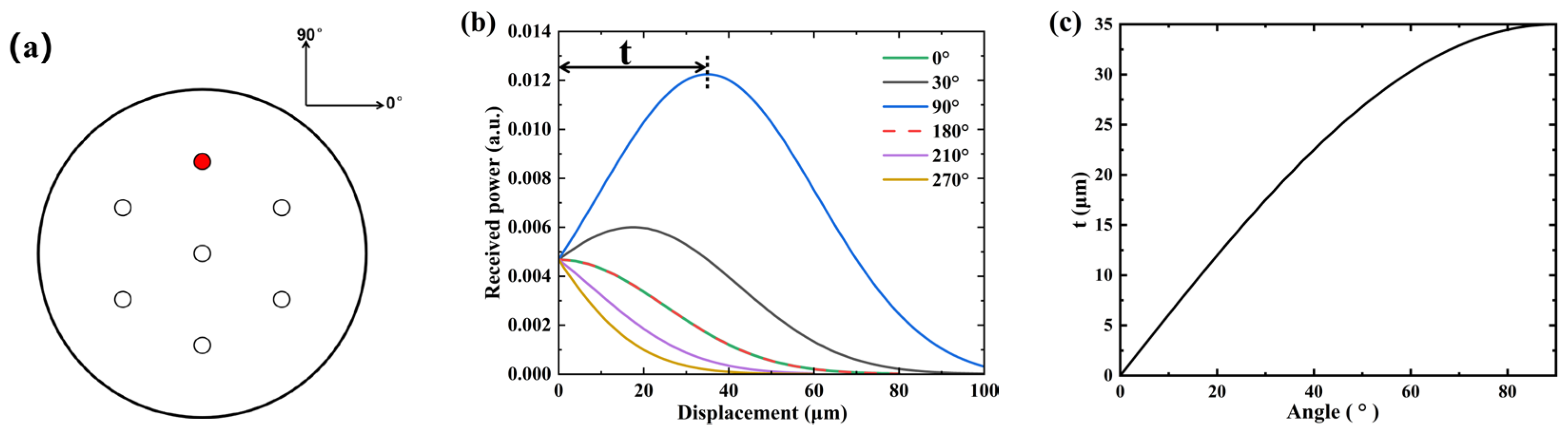Figure 3 illustrates the numerical model of the two-dimensional displacement. Core ① is marked in red to indicate that only 1540 nm light is input into core ①. During the simulation, the distance, d, between the SCF and the SMF was first altered to maximize the power received by the SMF.

The displacement direction was determined according to the angle definition provided in Figure 4a. Figure 4b presents the received power by the SMF when it moves along the directions of 0°, 30°, 90°, 180°, 210°, and 270°. It can be observed from the figure that when the SMF moves along the directions of 0°, 180°, 210°, and 270°, the power received by the SMF decreases. However, the rate of decrease varied depending on the direction of movement. When the SMF moved along the 30° and 90° directions, the power first increased and then decreased. The distance, t, at which the power transitioned from increasing to decreasing is related to the angle, and Figure 4c illustrates the relationship between the distance, t, and the angle. When the SMF moved along the 30° direction, the power initially increased, and after moving 17.5 μm, the power began to decrease. In contrast, when moving along the 10°direction, the power started to decrease after moving 6.08 μm. Therefore, the ability to discern power variations determines the angular resolution. Using a high-stability light source to reduce power fluctuations helped improve the displacement resolution capability.

In actual use, in addition to the 1540 nm light in core ①, cores ⑤ and ⑥ were, respectively, fed with 1530 nm and 1520 nm light, and the SMF received the light of these three wavelengths. During the simulation process, by combining the results at different angles, one could obtain the power variation for each wavelength received by the SMF as it moved in a certain direction. Figure 5 gives the results when the SMF moves along the directions of 30°, 180°, and 210°. As shown in Figure 5a, when the SMF moves along the 30° direction, the power variation of the 1540 nm light emitted by core ① and the 1520 nm light emitted by core ⑥ is the same, both initially increasing and then decreasing. When the SMF moved to the midpoint between cores ① and ⑥, the power of the light was at its maximum; if it continued to move, the power of these two wavelengths decreased. With the increase in displacement, the power of the 1530 nm light emitted by core ⑤ and received by the SMF gradually decreased. As shown in Figure 5b, when moving along the 180° direction, the power of 1540 nm and 1520 nm light decreased, while the 1530 nm light first increased and then decreased.

Table 1. The relationship between power variation for various wavelengths and displacement directions.

		1520 nm	1530 nm	1530 nm	Displacement Direction
Power Variation
					0°~60°
					60°~120°
					120°~180°
					180°~240°
					240°~300°
					300°~360°

provides the variation in light power at different wavelengths with the movement direction of the SMF. If the power of 1540 nm and 1520 nm increased while the power of 1530 nm decreased, the displacement direction was between 0° and 60°. If the power of 1540 nm increased while the power of 1530 nm and 1520 nm decreased, the displacement direction was between 60° and 120°. Similarly, other displacement directions could be determined. As shown in Figure 4, when the SMF moves along the 30° directions, the power first increases and then decreases. The distance, t, at which the power transitioned from increasing to decreasing is related to the angle, and Figure 4c illustrates the relationship between the distance, t, and the angle. If the direction of displacement is confirmed according to Table 1, the displacement range is related to the direction of movement. Figure 4c determines the range of displacement. When the SMF was moved along the directions of 30°, 180°, and 210°, its detection displacement range was 17.5 μm, 30 μm, and 35 μm, respectively.

4. Experimental Results and Discussion

Figure 6 is the experimental setup diagram of the proposed two-dimensional displacement sensor. Figure 6a is a microscope image of the end-face of the SCF (SM-7C1500, Fibercore, Southampton, UK), with a core diameter of 6.1 μm and a spacing of 35 μm between the cores. Figure 6b is a schematic diagram of the experimental setup. Light with wavelengths of 1520 nm, 1530 nm, and 1540 nm was incident on the three cores of the SCF. The SMF (SMF-28e, Corning, New York, NY, USA) was connected to the spectrometer (AQ6370D, YOKOGAWA, Tokyo, Japan) to display the power of the received three wavelengths of light. The three wavelengths of light originate from a super-radiant light diode (SLD, ASLD-CWDM-5, Amonics, Hong Kong, China), and specific wavelengths were selected through the use of three fiber Bragg gratings. During the experiment, a stepping motor with a precision of 8 nm controlled the movement of the SMF. The stepping motor can only move in one dimension. To achieve two-dimensional displacement measurement, the SCF was placed on a rotator, which could rotate 360° in the vertical plane to change the direction of displacement. The rotator was fixed on a high-precision five-axis displacement stage, which was used for the alignment of the SMF and the SCF. The SMF was fixed on another five-axis displacement stage through an optical fiber holder. Light at 1540 nm, 1530 nm, and 1520 nm wavelengths was used as the light source and input separately into cores ①, ⑤, and ⑥ of the SCF through a fan-in device. These three wavelengths of light were transmitted independently within their respective cores, and after emerging from the other end of the SCF, they were transmitted through the air to the end-face of the SMF. The SMF was connected to a spectrometer. When the distance between the SCF and the SMF was appropriate, the SMF received light of the three wavelengths. The direction of displacement was determined by judging the change in the power of light at each wavelength.

In the experiment, the SCF was first aligned with the SMF, and the alignment process was divided into the following three steps. (1) The SCF and the SMF were placed in close proximity and kept fixed. By using a fan-in device, 1550 nm light was input into the central core of the SCF. The five-axis displacement stage was moved to maximize the power received by the SMF. (2) The distance between the SCF and the SMF affected the power of the light received by the SMF. Using a fan-in device, 1540 nm light was input into core ① of the SCF, and the distance, z, adjusted to maximize the light power received by the SMF. Figure 6c shows the relationship between the received power and the distance, z. As the distance increased, the light power received by the SMF gradually increased, reaching a maximum when the distance was 580 μm. During the experiment, the position where the power was at its maximum was maintained. (3) The distance, z, was kept constant, 1550 nm light was re-input into the central core, and the five-axis displacement stage was fine-tuned to maximize the power received by the SMF, ensuring that the SCF was perfectly aligned with the SMF. This completed the alignment process between the SCF and SMF. It is worth noting that during the experiment, it was generally possible to make the two fiber end-faces parallel. Due to the cutting angle of optical fibers, the end-faces of the single-mode fiber and seven-core fiber were generally not perpendicular to the long axis of the fiber.

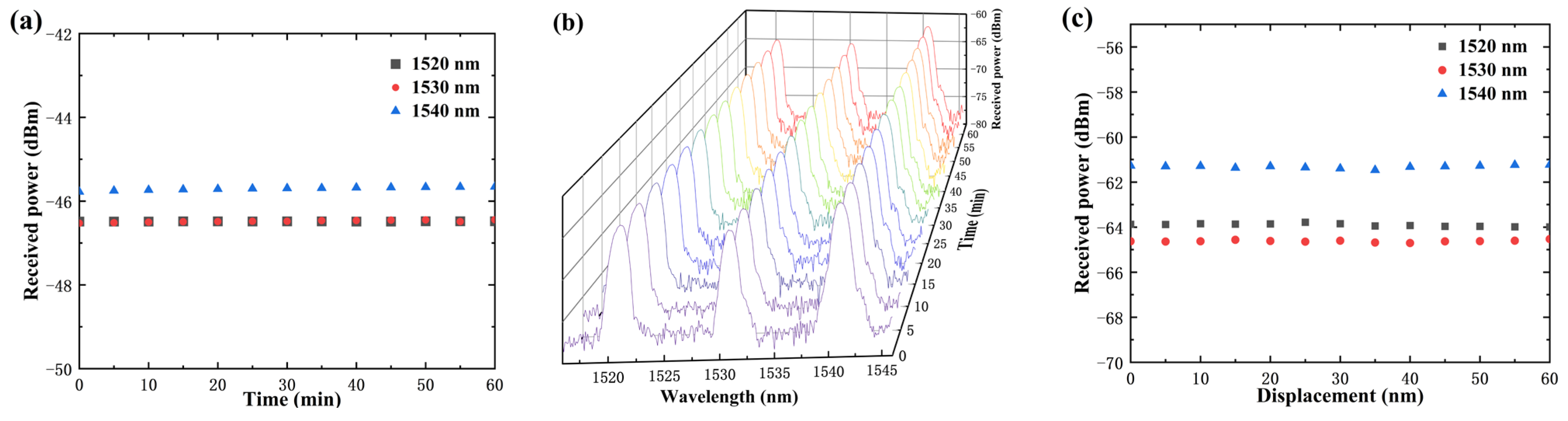
The power stability of the light source severely affected the performance of the sensor. At the beginning of the experiment, the stability of the 1520 nm, 1530 nm, and 1540 nm light sources was measured. Spectral information was recorded every 5 min for a total of 60 min. Figure 7a shows the power read by the spectrometer. Within 1 h, the power fluctuations of the 1520 nm, 1530 nm, and 1540 nm light sources were 0.076 dB, 0.085 dB, and 0.123 dB, respectively.

To verify the stability of the experimental setup, we also measured the power variation in light at different wavelengths received by the SMF after the SCF was aligned with the SMF. Figure 7b shows the results of repeated spectral scans, and Figure 7c shows the power variation read by the spectrometer. Within 1 h, the power fluctuations of 1520 nm, 1530 nm, and 1540 nm were 0.206 dB, 0.174 dB, and 0.238 dB, respectively. The experimental setup had excellent stability.

Figure 8 depicts the variation in power for different wavelengths received by the SMF when it was moved along the 30°, 90°, and 180° directions. Figure 8(a1,b1,c1) represents the spectral data captured by the spectrometer, whereas Figure 8(a2,b2,c2) corresponds to the associated power. When the SMF was moved along the 30°, 90°, and 180° directions, the experimental results were in good agreement with the simulated outcomes compared to Figure 5.

According to Table 1, the direction of displacement within a 60° range could be confirmed based on the changes in the power of the three wavelengths. When the direction of movement was less than 60°, the power of the 1520 nm light increased. When the direction of movement was greater than 60°, the power of the 1520 nm light decreased. During the experimental process, the 60° direction could be confirmed with a judgment error of less than 5°. In the experiment, due to the limitation in the number of available light sources, only three of the six surrounding cores were utilized, with the remaining three cores left unengaged. If all six surrounding cores were to be employed, the direction of displacement within a 30° range could be more accurately determined based on the observed power changes across these six cores.

The sensor’s sensitivity was analyzed as the SMF moved in the 210° direction. Figure 9a depicts the power variation at each wavelength, measured by the spectrometer, with the SMF moving in increments of 1 μm over a total distance of 10 μm. The top of the spectra in Figure 9a shows clear oscillatory structures. The spectra were then smoothed, as depicted in Figure 9b, and the maximum value of the smoothed curve was recorded as the power. Experimental observations indicate that the oscillatory structure became less pronounced with increasing power received by the SMF. When the power was sufficiently high, the spectrum became very smooth, suggesting that employing a higher power light source can mitigate spectral oscillations. Figure 9c demonstrates the correlation between the power read from the spectra and the displacement. As illustrated in Figure 9c, different wavelengths displayed varying sensitivities. The sensor’s sensitivity at 1520 nm, 1530 nm, and 1540 nm were 0.277 dB/μm 0.170 dB/μm 0.253 dB/μm, respectively. Figure 9d illustrates the spectral changes when the SMF was moved in increments of 200 nm, with the movement range extending from 5.2 μm to 6.2 μm. Figure 9e provides a partial enlargement of the image for clarity. Figure 9f displays the power readings corresponding to the spectra. The sensitivities at 1520 nm, 1530 nm, and 1540 nm were 0.34 dB/μm, 0.40 dB/μm and 0.36 dB/μm, respectively. In comparison to Figure 9c, the sensor exhibited varying sensitivities. The observed difference in sensitivity between Figure 9c,f could be attributed to the instability of the light source power.

It should be noted that the light emitted by the laser follows an approximate Gaussian distribution. For a certain wavelength, only the partially displaced region could be approximated as linear [25]. Generally, during the experimental process, one of the three wavelengths of light was situated in the linear region of the Gaussian spot. Initially, the direction of displacement was determined based on the variations in power at each wavelength. Subsequently, the appropriate sensitivity was selected based on the trend of the power changes in that direction.

Reference [3] describes a fiber Bragg grating displacement sensor with a sensitivity of 3304 pm/mm, and the accuracy was only 20 μm. Reference [25] describes a micro-displacement sensor based on a cantilever. A photodetector was utilized to measure the power received by the cantilever, achieving nanometer-level detection precision. The detection accuracy of the sensor was very high. However, the detector could only provide displacement information in one direction. Reference [12] proposes a 2D displacement sensor based on macro-bending loss and the optical power coupling effect, and the sensitivity was reported to be 2.6 nW/mm. The highest power received during the experiment was about −61.9 dBm, and the direction of displacement could be determined when the movement step was 200 nm. A power meter can generally distinguish power in the nW range. If a higher power light source is used, the sensor can detect displacements of tens or even several nanometers.

5. Conclusions

We propose a two-dimensional displacement sensor, characterized by high precision, simple structure, and convenient implementation. By aligning a section of the SCF with a segment of the SMF, a two-dimensional displacement sensor was formed. When light at 1520 nm, 1530 nm, and 1540 nm was introduced into the three side cores of the SCF, the SMF could receive light at these three wavelengths. As the position of the SMF shifted, the received optical power changed, and the direction of displacement could be determined based on these variations. Utilizing the three side cores of the SCF allowed for direction determination within a 60° range. When the SMF was moved in increments of 200 nm, with the movement range extending from 5.2 μm to 6.2 μm, the sensitivities at 1520 nm, 1530 nm, and 1540 nm were 0.34 dB/μm, 0.40 dB/μm and 0.36 dB/μm, respectively. Employing additional side cores and higher power light sources can further enhance the detection precision. This displacement sensor has the potential for application in various fields, including the structural health monitoring of buildings and high-precision alignment in the semiconductor industry.