Abstract
In this paper, we explore the enhancement of a 4.6 km dual-polarization 2 × 2 MIMO D-band photonic-assisted terahertz communication system using iterative pruning-based deep neural network (DNN) nonlinear equalization techniques. The system employs advanced digital signal processing (DSP) methods, including down-conversion, resampling, matched filtering, and various equalization algorithms to combat signal distortions. We demonstrate the effectiveness of DNN and iterative pruning techniques in significantly reducing bit error rates (BERs) across a range of symbol rates (10 Gbaud to 30 Gbaud) and polarization states (vertical and horizontal). Before pruning, at 10 GBaud transmission, the lowest BER was 0.0362, and at 30 GBaud transmission, the lowest BER was 0.1826, both of which did not meet the 20% soft-decision forward error correction (SD-FEC) threshold. After pruning, the BER at different transmission rates was reduced to below the hard decision forward error correction (HD-FEC) threshold, indicating a substantial improvement in signal quality. Additionally, the pruning process contributed to a decrease in network complexity, with a maximum reduction of 85.9% for 10 GBaud signals and 63.0% for 30 GBaud signals. These findings indicate the potential of DNN and pruning techniques to enhance the performance and efficiency of terahertz communication systems, providing valuable insights for future high-capacity, long-distance wireless networks.
1. Introduction
Modern communication networks face unprecedented challenges, requiring larger bandwidth, higher speed, and more flexible service capabilities []. The terahertz (THz) frequency band (0.1 THz–10 THz) is a promising candidate for future 6G communication because of its vast spectrum resources and high-speed data transmission potential. However, traditional electronic devices struggle with bandwidth limitations in generating and processing high-bit-rate THz signals []. Photonic-assisted THz signal generation technology has emerged, overcoming these limitations and enabling ultra-wideband and high-capacity data transmission.
In the exploration of the THz band, Radio-over-Fiber (RoF) technology has garnered widespread attention because of its ability to combine the high bandwidth of fiber optics with the flexibility of wireless communication. RoF technology modulates wireless signals onto optical carriers, utilizes fiber optics for long-distance transmission, and then converts the optical signals back to wireless signals at the wireless access point, thereby enabling high-speed wireless communication []. An experiment in 2012 achieved 24 Gbit/s ASK signal transmission at the 300 GHz band []. Subsequently, researchers widely introduced PS, MIMO, PDM, and Few-subcarrier OFDM technologies, significantly improving the transmission rate of RoF systems [,,]. Extensive experiments conducted across various bands demonstrate the potential of each band in enhancing RoF system transmission performance [,,]. Notably, Li W et al. achieved 4.6 km wireless transmission in the D-band in 2022, setting a record for the longest transmission distance []. These studies provide valuable experience and data support for the application of RoF systems across various bands.
However, RoF systems may suffer from various nonlinear effects, which affect system performance, especially at high bit rates and high spectral efficiencies. Previously, researchers mostly used traditional equalization algorithms such as Decision Feedback Equalizer (DFE), Least Mean Square (LMS), and Volterra to handle nonlinearity [,,,]. In recent years, researchers have improved these algorithms to suit different systems. Specifically, using the MIMO structure Volterra nonlinear equalization (VNE) algorithm, Wei Y et al. successfully transmitted 25-Gbaud 16-QAM signals over a 4.6 km 2 × 2 MIMO wireless system at the 125 GHz D-band in 2023, achieving a minimum BER of 2.05 × 10⁻² [].
However, these improved traditional equalization algorithms have limited capabilities. To address these limitations, the use of machine learning (ML) technology in RoF systems has been proposed and has become an active research area []. Unlike traditional methods, ML methods learn system impairments from training data. Compared with traditional signal processing methods, ML-based schemes consider and handle all impairments simultaneously, as well as the interactions between different types of impairments. Researchers have experimented with and applied various types of ML methods. In the non-neural network domain, researchers achieved 6 GHz RoF transmission using the k-means algorithm in 2010 []. Subsequently, researchers improved the performance of the k-means algorithm in 6 GHz RoF systems using the Fuzzy c-means Gustafson–Kessel (FCM-GK) algorithm []. Researchers also verified the effectiveness of the k-nearest neighbors (KNN) algorithm and support vector machine (SVM) in reducing BER in RoF systems under single-channel and single-polarization conditions [,]. In 2017, SVM was applied to a single-carrier 2.4 Gbps 56.2 GHz RoF system []. In 2020, researchers proposed and validated the effectiveness of a deep reinforcement learning (DRL) method based on the proximal policy optimization (PPO) algorithm, which can be effectively extended to MIMO systems []. Non-neural network algorithms have only been validated in simulations and low-speed, short-distance RoF systems. Neural networks have been more maturely applied in high-speed, long-distance RoF systems. Researchers have verified that neural network algorithms significantly outperform traditional algorithms in handling nonlinear effects in RoF systems []. In 2017, researchers demonstrated the advantage of DNN over VNLE in a 5 Gbps 60 GHz RoF system []. In 2020, researchers began applying convolutional neural networks (CNNs) and Binary Convolutional Neural Networks (BCNNs) to a 5 Gbps 60 GHz RoF system []. In recent years, researchers have improved DNN and CNN algorithms, introducing complex-valued neural networks (CVNNs) and 2D-CNN to achieve equalization of complex signals in RoF communication systems. These algorithms further reduced the BER of DNNs and CNNs [,]. Subsequently, researchers applied complex neural networks to dual-polarization systems, achieving transmission below the hard decision forward error correction (HD-FEC) BER threshold in a 30 GBaud 320 GHz THz system []. In the latest research, Recurrent Neural Networks (RNNs) and Long Short-Term Memory (LSTM) have also been introduced for signal equalization in RoF systems [,].
To balance BER performance and computational complexity, we note that DNNs have significantly lower complexity than CNNs, RNNs, and LSTM when handling the same tasks []. Researchers have shown that a three-layer DNN is sufficient to solve nonlinear problems in RoF systems []. Pruning techniques can further reduce BER and computational complexity, making pruned DNNs have lower complexity than Volterra [].
Therefore, in this paper, we construct a 4.6 km long-distance dual-polarization 2 × 2 MIMO D-band photonics-assisted THz communication system. Innovatively applying DNN neural networks combined with iterative pruning techniques to the RoF system, we successfully reduced the BER of 10 Gbaud to 30 Gbaud 16QAM signals below the HD-FEC threshold of 3.8 × 10⁻³, increasing the transmission rate from 10 Gbaud to 30 Gbaud compared with the MIMO Volterra nonlinear equalization (MIMO-VNLE) algorithm. Meanwhile, iterative pruning techniques significantly reduced the complexity of the DNN. For 10 Gbaud data, complexity could be reduced by up to 85.9%, and for 30 Gbaud data, by up to 63.0%. The innovative combination of DNN and iterative pruning techniques not only enhances system performance but also provides new ideas and technical paths for the design and optimization of future communication systems.
This paper consists of five parts. The next four parts are as follows: Section 2 details the technical principles of the experiment. Section 3 introduces the experimental setup of the dual-polarization photonics-assisted THz wireless transmission link. Section 4 presents the experimental results of neural networks and iterative pruning and conducts in-depth discussions. Section 5 summarizes the main findings and conclusions of this study.
2. Principle
2.1. Photonics-Assisted MIMO Terahertz Technology
Figure 1 illustrates the principle of photonic-assisted terahertz signal generation based on heterodyne beat frequency. Two independent continuous-wave lasers are employed, one serving as the signal laser and the other as the local oscillator (local oscillator, LO) laser. These lasers emit light waves with distinct frequencies. The output of the signal laser is modulated by the optical modulator (Opt. Mod), which is used to encode information onto the optical carrier. The modulated signal light wave is then coupled with the unmodulated local oscillator light wave using an optical coupler (OC). The coupled light waves are transmitted through single mode fibers (SMFs) before reaching the photodetector (PD). Within the PD, the interaction between the signal light wave and the local oscillator light wave, because of the PD’s quadratic-law characteristic, generates a beat frequency signal, whose frequency is equal to the difference between the two light wave frequencies. If this difference falls within the terahertz frequency range, the resulting beat frequency signal is a terahertz wave. In this manner, a terahertz signal can be directly generated within the PD without the need for additional electrical terahertz wave generation devices. The high-gain antenna (HA) is used to transmit the generated terahertz signal, ensuring efficient signal propagation.
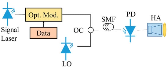
Figure 1.
Photonics-assisted terahertz technology based on heterodyne beat frequency.
Within the photodetector (PD), the phenomenon of beat frequency can be described by the following formulas. Suppose two light waves are heterodyne beat after the PD, their optical fields can be expressed as follows:
where Ei(t) represents the optical field of the i-th light wave, Ei0 is its amplitude, ωi is its angular frequency, and ϕi is its phase. When these two light waves are coupled into the PD, the output current I(t) of the PD is proportional to the square of the incident light power, that is,
Among these terms, the intermediate term can be expanded into the following:
where the first term represents the beat frequency component and the second term represents the sum frequency component. If the difference between ω1 and ω2 falls within the terahertz frequency range, then the beat frequency component is a signal of terahertz frequency. This is the principle by which the PD generates a beat frequency.
The photonic-assisted terahertz signal generation technology based on the heterodyne beat frequency scheme boasts high flexibility and tunability, capable of generating both broadband terahertz waves, suitable for a variety of application scenarios. The advantages of this technology include high efficiency, ease of integration and control, as well as the ability to operate at room temperature.
Polarization multiplexing is a technology that utilizes the polarization characteristics of electromagnetic waves to increase the capacity of communication systems. In polarization multiplexing, two or more signals with different polarization directions can be transmitted simultaneously within the same frequency band without interfering with each other, thereby enhancing spectral efficiency. MIMO technology is a technique that employs multiple antennas for both transmission and reception, improving the performance of wireless communication systems through spatial diversity and spatial multiplexing.
In our system, we utilize photonic-assisted terahertz technology combined with polarization multiplexing MIMO technology to establish a 2 × 2 MIMO wireless link with two transmitters and two receivers. Figure 2a is a schematic diagram of the polarization multiplexed 2 × 2 MIMO wireless transmission system, where H and V represent horizontal and vertical polarization directions, respectively. Figure 2b is a schematic diagram of the traditional 2 × 2 MIMO wireless transmission system, where two wireless links transmit signals in the same polarization direction.
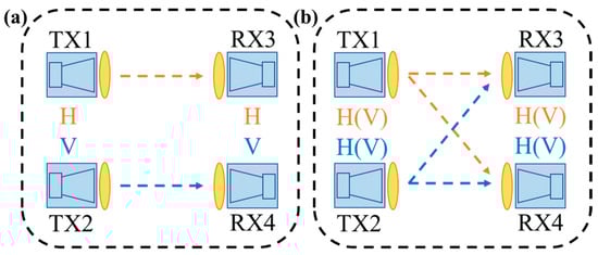
Figure 2.
Schematic diagrams of 2 × 2 MIMO wireless transmission systems. (a) Traditional 2 × 2 MIMO. (b) Polarization multiplexed 2 × 2 MIMO.
2.2. Neural Network Nonlinear Equalizer
In fiber-wireless communication systems, nonlinear noise is difficult to mitigate using traditional polarization demultiplexing techniques. Considering the excellent nonlinear fitting capabilities of neural networks, we propose applying neural network algorithms as an adaptive algorithm in polarization demultiplexing systems.
In our experiment, we employ a DNN with three fully connected layers (FCLs), which include batch normalization (BN), the rectified linear unit (ReLU) activation function, the mean squared error (MSE) loss function, and the Adam optimizer. The batch normalization layer normalizes the output of the fully connected layers to prevent distribution skewing and gradient vanishing. Normalization is achieved by calculating the mean and variance of each mini-batch of data, followed by scaling and shifting the data. The ReLU activation function performs a nonlinear transformation on the batch-normalized data, with the following formula:
The mean squared error (MSE) loss function is used to measure the discrepancy between the network’s predicted values and the actual values. The formula for MSE is as follows:
where d(n) represents the actual value, y(n) is the output data from the neural network, and N is the batch size. Adam (Adaptive Moment Estimation) is an adaptive learning rate optimization algorithm that adjusts the learning rate for each parameter during training to improve convergence speed and stability.
This three-layer DNN neural network, through the backpropagation algorithm and the Adam optimizer, continuously adjusts the weights and biases during training to minimize the MSE loss function, thereby enhancing the prediction accuracy. By introducing neural network algorithms for THz-wave channel equalization, we can leverage the powerful fitting capabilities of neural networks to overcome the limitations of traditional algorithms under complex channel conditions, compensate for channel distortion, and achieve higher transmission performance.
2.3. Iterative Neural Network Pruning Technology
Although neural networks are powerful, they always consume a large amount of storage, memory bandwidth, and computational resources. Neural network pruning is an optimization technique aimed at reducing the complexity of the network by removing certain weights or neurons, thereby improving runtime efficiency, reducing storage requirements, and sometimes enhancing generalization capabilities. The key steps of pruning are as follows: (1) Train a complete neural network until it reaches a satisfactory performance level on the training data. This initial network usually has more weights and neurons than actually needed. (2) Determine a criterion to decide which weights or neurons should be removed. (3) Based on the selected criterion, rank the weights or neurons in the network and remove those deemed unimportant. (4) Retrain the network to fine-tune the remaining weights, adapting them to the new network structure. This step helps to recover the performance that may have been lost by pruning.
In data processing, we used threshold-based pruning, with the standard deviation (standard deviation, STD) as the measure. The basic idea of this method is that the distribution of weight values typically revolves around a central value (such as the mean) with a certain degree of dispersion, which can be measured by the standard deviation. A larger standard deviation indicates a more dispersed distribution of weight values, while a smaller standard deviation indicates a more concentrated distribution. Therefore, in step (3), for each weight matrix (each layer) in the network, the standard deviation of its weight values is calculated. A threshold for the standard deviation is set, which is a relative value to the layer’s standard deviation. That is, threshold = threshold ratio × standard deviation. Weights with a standard deviation below the set threshold are set to 0, completing the removal of weights.
For each weight matrix, a weight value’s standard deviation below the set threshold means that these weights have relatively smaller changes compared with other weights and may contribute less to the network’s output. Therefore, removing those weights with a standard deviation below the set threshold.
Iterative pruning allows the network to adapt gradually to the changes brought by pruning. After each pruning, the network is retrained to ensure its performance does not drop sharply. One-time pruning may lead to over-pruning, i.e., removing too many important weights, which can severely harm the network’s performance. Iterative pruning avoids this situation by pruning gradually, ensuring that the network can still function normally after each pruning. Moreover, iterative pruning helps explore the optimal network structure. Through multiple iterations, different pruning strategies and degrees can be tried, eventually finding a network structure that is efficient and performs well. Figure 3 is a schematic diagram of the iterative pruning process for QAM.
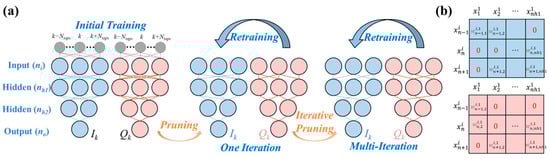
Figure 3.
(a) Schematic diagram of the iterative pruning process. (b) Weight matrix diagram of pruning in the fully connected layer.
As depicted in Figure 3, for the 16QAM signal, we employ an I/Q separation approach, decomposing the 16QAM signal into two independent signals, each of which is then equalized using a neural network. Given that the I and Q path signals may experience different distortions and noise effects during transmission, handling them separately allows for the design of more suitable equalizers tailored to the characteristics of each path, thereby enabling more precise compensation for specific distortions on each path and enhancing overall equalization performance.
3. Experimental Setup
Figure 4a illustrates a 4.6 km 2 × 2 MIMO photonic-assisted terahertz communication system in the D-band. At the transmitter, offline baseband signals are first generated via MATLAB and loaded into a 120 GSa/s arbitrary waveform generator (AWG) to produce 16QAM signals with varying symbol rates. These signals are then amplified by two parallel electrical amplifiers (EAs) with a gain of 25 dB and modulated using an I/Q modulator with a 3 dB bandwidth of 30 GHz. An external cavity laser-1 (ECL1) at a wavelength of 1550 nm serves as the optical carrier and has 12 dBm optical power. The modulated signal is amplified by a polarization-maintaining erbium-doped fiber amplifier (PM-EDFA) and coupled with a 14.5 dBm LO optical source emitted by laser 2 (ECL2) at a wavelength of 1551.1 nm. Both the external cavity lasers have a linewidth of 100 kHz. The signal is transmitted in two polarization directions. After transmission through 100 m of SMF-28 fiber, the signal’s optical power is adjusted by a variable optical attenuator (VOA) and then split into two paths by PM-OC2. To eliminate correlations between the signal paths effectively, a 2 m long polarization-maintaining optical delay line (PM-ODL) is added to one path. The optical signals of the two paths, after transmission through a 1 m polarization-maintaining fiber, are input into UTC-PD1 and UTC-PD2, respectively. These devices operate within a frequency range of 110 to 170 GHz and generate a 124.8 GHz sub-terahertz signal through optical mixing technology. Because of the rapid attenuation of sub-terahertz band signals during free-space transmission, the signal is amplified by a cascade of LNA1/LNA3 with a gain of 18 dB and PA1/PA2 with an output power of 13 dBm to support a wireless transmission distance of 4600 m. Subsequently, the amplified terahertz signal is transmitted via a pair of high-gain antennas (HAs) with horizontal/vertical polarization (H-/V-pol.), each with a gain of 25 dBi. Given the small aperture of high-gain antennas in the sub-terahertz band, a pair of plano-convex lenses (Lens1/Lens3 and Lens2/Lens4) is used to focus the terahertz beam to maximize the reception power at the receiving-end HAs. Specifically, the diameters of Lens1/Lens2 and Lens3/Lens4 are 10 cm and 60 cm, respectively.
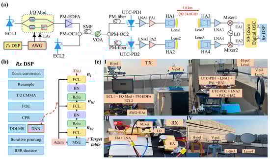
Figure 4.
(a) Schematic diagram of a 4.6 km 2 × 2 MIMO photonic-assisted terahertz communication system architecture in the D-band; (b) flowchart of the digital signal processing at the receiving end; and (c) the 4.6 km 2 × 2 MIMO photonic-assisted terahertz experimental setup. (I) Transmitter, before single-mode fiber, (II) transmitter, after single-mode fiber, (III) receiver, signal processing, and (IV) receiver, lens.
After 4.6 km wireless transmission, the sub-terahertz signal is focused by Lens3/Lens4 and received by H-/V-pol. HAs. The received H-/V-pol. signals are amplified by LNA2/LNA4 with a gain of 33 dB and down-converted by Mixer1/Mixer2. The local oscillator (LO) operates at 112 GHz, generating a 12.8 GHz intermediate frequency (IF). After down-conversion, the IF signals are amplified by EA3/EA4 with a gain of 26 dB and captured by an 80 GSa/s digital storage oscilloscope (DSO). During the experiment, a high-power telescope was used to assist alignment, which helped improve the accuracy and efficiency of alignment. The transmitter and receiver are located in two campuses of Fudan University, with the transmitter on the rooftop of Guanghua Tower at an altitude of 142 m, and the receiver on the rooftop of the Physics Building. They are 4.6 km apart.
Figure 4b shows the channel equalization process at the receiving end of the dual-polarization system. The DSP flow at the receiving end includes down-conversion, resampling, matched filtering, T/2 constant modulus algorithm (CMA), frequency offset estimation (FOE), carrier phase recovery (CPR), direct detection least mean square (DD-LMS) equalization, and DNN-based neural network equalization. First, the IF signal is down-converted and resampled to the baseband. Next, CMA linear equalization and DD-LMS are used to compensate for inter-symbol interference (ISI) caused by channel propagation characteristics. FOE compensates for frequency drift effects due to the laser frequency offset, while CPR reduces phase noise introduced by the laser linewidth. Subsequently, the dual DNN decomposes the complex QAM architecture into independent I and Q paths and performs deep equalization on each.
Figure 4c illustrates the iterative pruning process for the neural network. Pruning the I and Q networks of the dual DNN architecture to varying degrees can eliminate redundancy as much as possible while compensating for the imbalance between the I/Q paths to some extent.
4. Experimental Results and Discussion
Figure 5 shows the spectrum of sub-terahertz 16QAM signals with sampling rates of 80 GHz, intermediate frequencies of approximately 12.8 GHz, and baud rates of 10 Gbaud, 20 Gbaud, and 30 Gbaud, respectively.
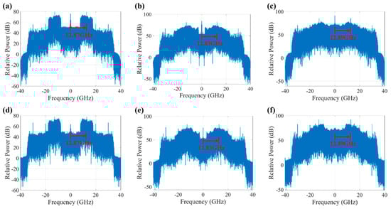
Figure 5.
Signal spectra: (a) V-pol-10 Gbaud, (b) V-pol-20 Gbaud, (c) V-pol-30 Gbaud, (d) H-pol-10 Gbaud, (e) H-pol-20 Gbaud, and (f) H-pol-30 Gbaud.
From the spectral diagrams, it is evident that the signal spectrum shifts upward at different baud rates, specifically showing that the actual frequency is slightly higher than the anticipated 12.80 GHz. This phenomenon may be attributed to the phase noise and frequency instability caused by the laser linewidth. A larger laser linewidth leads to higher phase noise, which increases the phase noise in the beat frequency signal, subsequently causing frequency drift and jitter. It could also be due to insufficient frequency stability in the laser itself, resulting in an output frequency higher than expected, possibly caused by internal noise or temperature fluctuations. Additionally, frequency-selective fading in fiber transmission or terahertz channels may also cause the spectrum to shift upward. These factors increase inter-symbol interference (ISI) and phase errors, impacting the accuracy of signal demodulation and increasing the BER. Therefore, advanced DSP algorithms need to be employed at the receiving end to compensate for these effects and improve the BER.
At the receiving end, we employed traditional DSP demodulation methods. The BERs obtained for the 10 Gbaud, 20 Gbaud, and 30 Gbaud signals in both polarization directions after applying DDLMS were 0.0426, 0.0362, 0.0773, 0.0776, 0.1826, and 0.1856, respectively. After applying the MIMO-VNLE, the BERs were measured as 0.00392, 0.00378, 0.00843, 0.00827, 0.0221, and 0.0192, respectively. Since the results of the MIMO-VNLE did not meet the hard decision threshold requirements, we employed a three-layer neural network after the DDLMS to further reduce the BER. The network structure was ni-360-260-1, meaning the first layer had 360 neurons, the second layer had 260 neurons, and the output layer had 1 neuron. The data length was 98304, and the length of the training data was 32768.
By analyzing Figure 6, we discern the neural network’s convergence trend, and note that the average loss for the 30 Gbaud data is initially significantly higher than that for the 10 Gbaud and 20 Gbaud data, but eventually, the average loss for all three rates converges to a similar level. This phenomenon arises because data with higher baud rates exhibit more complex signal characteristics and noise patterns, resulting in higher initial losses. Consequently, the network requires more time at the outset to adapt to these features associated with higher baud rates. As training progresses, the network gradually learns to handle the characteristics of high-baud-rate data by adjusting its weights and parameters, leading to a reduction in loss until the average losses for all rates converge to a similar level. This indicates that the network is capable of effectively processing data at different rates while maintaining stable performance. Such convergence underscores the network’s robust generalization capabilities and adaptability.
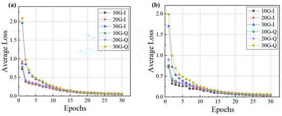
Figure 6.
Neural network training epochs vs. average loss. (a) V-pol and (b) H-pol.
After processing with a three-layer neural network, the calculated BERs were 0.0025, 0.0021, 0.0081, 0.0063, 0.0093, and 0.0121, respectively. The results show that the BER for the 10 Gbaud data reached the HD-FEC threshold of 3.8 × 10⁻³, while the BERs for the 20 Gbaud and 30 Gbaud data reached the 20% SD-FEC threshold at 2.0 × 10⁻³. The neural network demonstrated significant effectiveness in processing signals for the 2 × 2 MIMO D-band photonic-assisted terahertz communication system, providing an effective means to improve system performance.
However, during the training process, to capture complex patterns and features in the data, the network learns a large number of weights and neurons. Some of these weights and neurons may be redundant, meaning they can be removed without significantly affecting the network’s performance. Pruning, as an optimization technique, can reduce the network’s complexity by removing these redundant weights and neurons, thereby lowering storage requirements, reducing computational resource demands, and improving runtime efficiency and generalization capabilities.
Figure 7 illustrates the network sparsity results of a three-layer DNN neural network after iterative pruning, using V-pol as an example. We employed a standard deviation-based weight pruning method, with each pruning round followed by 10 learning epochs, and set a threshold ratio of 0.8, where the pruning threshold equals the threshold ratio multiplied by the standard deviation. After 20 iterations, we observed that the model’s sparsity gradually converged. Notably, the sparsity of the I path after pruning was approximately 8% higher than that of the Q path, and it significantly decreased with increasing signal rate. This is attributed to the fact that, during signal transmission, the Q path may have experienced more severe distortions and noise effects compared with the I path. The path differences between the I and Q paths led the neural network to process the I path data with more redundant information, hence exhibiting higher sparsity post-pruning. Additionally, as the signal rate increases, the network sparsity obtained through pruning decreases. This is because higher-rate signals are subject to greater inter-symbol interference and nonlinear effects during transmission, necessitating the retention of more weights by the network to capture these details, resulting in lower sparsity. Furthermore, we observed that the sparsity of the fc1 layer is significantly greater than that of the fc2 layer. This is likely because the fc1 layer serves as the initial layer of the network, potentially responsible for capturing more general features of the input signal, which are more redundant and thus more prone to pruning. In contrast, the fc2 layer may be responsible for more specific feature extraction, which is more critical to the network’s final output, so more weights are retained during pruning, leading to lower sparsity.
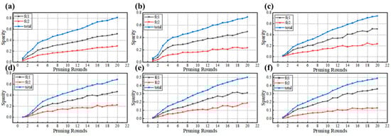
Figure 7.
V-pol neural network pruning rounds vs. sparsity: (a) 10 GBaud-I, (b) 10 GBaud-Q, (c) 20 GBaud-I, (d) 20 GBaud-Q, (e) 30 GBaud-I, and (f) 30 Gbaud-Q.
In Figure 8, we further explored the impact of varying threshold ratios (from 0.1 to 1.0) on the sparsity of I and Q path signals at different rates (10 Gbaud, 20 Gbaud, 30 Gbaud) and different polarization directions (V-pol and H-pol). The experimental results indicate that after 20 rounds of iterative pruning, the black and blue lines, representing the I path signals of V-pol and H-pol, respectively, exhibit significantly and consistently higher sparsity than the red and green lines, which represent the Q path signals, in agreement with the findings in Figure 7. Moreover, the sparsity of H-pol signals is notably greater than that of V-pol signals. This discrepancy is attributed to the distinct propagation characteristics of signals under different polarization states; for instance, in wireless communications, horizontally polarized signals may be more susceptible to ground reflections, whereas vertically polarized signals may be less sensitive to such reflections. Additionally, as the threshold ratio increases, the sparsity achieved through pruning initially rises and then declines. This phenomenon occurs because, at lower threshold ratios, fewer weights are removed in each pruning round, resulting in insufficient pruning. As the threshold ratio gradually increases, more weights are removed, leading to a gradual rise in sparsity. However, when the threshold ratio becomes excessively high, an excessive number of important weights may be removed, and these weights are likely to be restored during the retraining process, leading to redundancy. Hence, the sparsity begins to decrease.
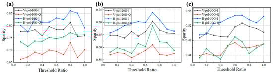
Figure 8.
Neural network pruning threshold ratio vs. sparsity: (a) 10 GBaud, (b) 20 GBaud, and (c) 30 GBaud.
Furthermore, we observed that different rates of signals achieve their maximum sparsity at distinct threshold ratios. Specifically, for 10 Gbaud signals, the threshold ratio is 0.8. For 20 Gbaud signals, the threshold ratio is 0.7. For 30 Gbaud signals, the I path threshold ratio is 0.7, and the Q path threshold ratio is 0.6. This variation is due to the fact that low-rate signals experience less inter-symbol interference and nonlinear effects, requiring fewer features from the network and containing more redundant weights that are easier to restore network performance during retraining, thus allowing for a higher pruning threshold. Conversely, for high-rate signals, the network requires more weights to capture the characteristics of the signals; hence, a lower pruning threshold should be applied. As mentioned in Figure 7, the I path signals experience significantly less inter-symbol interference and nonlinear effects compared with the Q path, and at a transmission rate of 30 Gbaud, the pruning threshold for the I path is greater than that for the Q path, further corroborating this observation.
In Figure 9, we further explore the impact of varying threshold ratios (from 0.1 to 1.0) on the BERs of signals at different rates (10 Gbaud, 20 Gbaud, 30 Gbaud) and different polarization directions (V-pol and H-pol), as well as the effect of retraining epochs (epochs = 5, 10, 15) after pruning on the BER trend. After 20 rounds of pruning, it was found that setting the retraining period to 10 epochs resulted in the lowest BER. This may be due to the fact that 10 epochs represent a balance point, allowing the network to maintain generalization capability while improving performance. For 10 Gbaud signals, the BER curve generally shows that as the threshold ratio increases, the BER gradually rises. At a threshold ratio of 0.1, the BER can be reduced by approximately 37%. However, as the threshold ratio increases, the BER gradually rises until it reaches the same level as before pruning at a threshold ratio of 0.8. For 20 Gbaud and 30 Gbaud signals, the BER first decreases and then increases with the rise in the threshold ratio. For 20 Gbaud signals, the minimum BER is achieved at a threshold ratio of 0.7. For 30 Gbaud signals, the minimum BER for V-pol signals is achieved at a threshold ratio of 0.7, while for H-pol signals, it is achieved at a threshold ratio of 0.6. At these threshold ratios, the minimum BERs after pruning are all around 2.5 × 10⁻³, meeting the hard decision threshold.
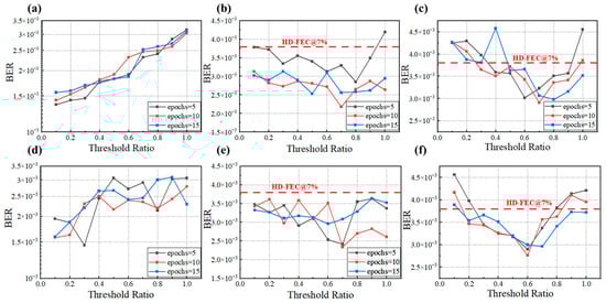
Figure 9.
Neural network pruning threshold ratio vs. BER: (a) V-pol-10 GBaud, (b) V-pol-20 GBaud, (c) V-pol-30 GBaud, (d) H-pol-10 GBaud, (e) H-pol-20 GBaud, and (f) H-pol-30 GBaud.
The gradual rise in BER for 10 Gbaud signals with an increasing threshold ratio may be because there are fewer features of low-rate signals, and the network before pruning has a certain degree of overfitting. Pruning eliminates these redundant weights, leading to an increase in the error rate, but this can enhance the network’s adaptability. For 20 Gbaud and 30 Gbaud signals, the BER first decreases and then increases because, at lower threshold ratios, the network accurately prunes weights that contribute less to the output and further optimizes the distribution of weights through retraining, thereby reducing the BER. However, when the threshold ratio is too high, too many important weights are removed and cannot be recovered during retraining, resulting in a decline in network performance and an increase in BER. Additionally, we can observe that after pruning, the error rate for H-pol signals is slightly lower than that for V-pol signals, which corroborates the analysis in Figure 8 that horizontally polarized signals may be more susceptible to effects during wireless propagation.
Figure 10 illustrates the impact of the entire pruning process on the BER, where PR_5 represents five pruning rounds, and so forth. The experimental results demonstrate that the DNN method can reduce the BER by an order of magnitude, while the pruning process further slightly reduces the BER. Specifically, through the combined application of DNN and pruning, we successfully achieved BERs below the HD-FEC threshold for signals ranging from 10 Gbaud to 30 Gbaud.
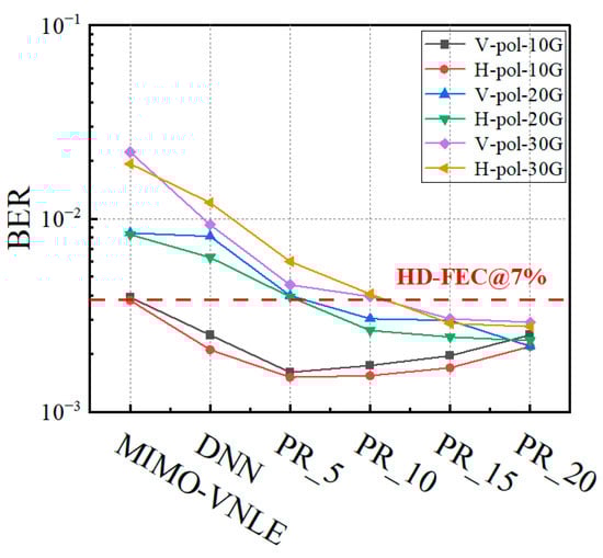
Figure 10.
Different equalization methods vs. BER.
This finding indicates that DNN has a significant effect in improving signal demodulation performance, and the pruning process further enhances performance by optimizing the network structure. This combined strategy provides an effective solution for high-efficiency and high-performance signal processing, especially in communication systems that require stringent BER requirements.
Table 1 and Table 2 present data indicating that, after pruning, the complexity reduction for H-pol is slightly greater than that for V-pol, and the complexity reduction for the I path signals is significantly greater than that for the Q path signals. For the 10 GBaud and 20 Gbaud data, iterative pruning techniques can reduce complexity by approximately 75%; for the high-rate 30 GBaud signals, iterative pruning techniques can reduce complexity by about 50%. Through pruning, we successfully reduced the number of network weights and significantly lowered computational complexity. These results demonstrate the effectiveness of pruning techniques in reducing network complexity, particularly when applied to signal processing at different polarization directions and different rates.

Table 1.
Complexity of V-pol before and after pruning.
Table 2.
Complexity of H-pol before and after pruning.
5. Conclusions
In this paper, we successfully constructed and tested a 4.6 km polarization-multiplexed 2 × 2 MIMO photonic-assisted terahertz communication system. The experimental results demonstrate that the synergistic approach of using DNN with iterative pruning based on the standard deviation can significantly reduce system complexity while maintaining or lowering the signal BER. We successfully reduced the BER of dual-polarization signals from 10 Gbaud to 30 Gbaud by more than an order of magnitude, meeting the HD-FEC threshold and achieving the transmission of a 124.8 GHz, 240 Gbps (30 Gbaud) PDM-16QAM signal. Furthermore, for 10 GBaud and 20 Gbaud data, complexity was reduced by approximately 70%. For 30 Gbaud data, complexity was reduced by about 50%. These results not only underscore the effectiveness of iterative pruning techniques in reducing BER and enhancing system performance but also emphasize their potential applications in practical communication systems. These findings are of significant importance for advancing the development of next-generation communication technologies.
Author Contributions
Conceptualization, J.L., S.X., Q.W., J.Z., J.G., S.W., Z.O. and Y.M.; data curation, W.Z.; formal analysis, J.L.; funding acquisition, J.Y. and W.Z.; investigation, J.L.; methodology, J.L.; project administration, W.Z.; resources, W.Z.; software, J.L.; supervision, W.Z.; validation, J.L.; visualization, J.L.; writing—original draft, J.L.; writing—review and editing, J.Y. and W.Z. All authors have read and agreed to the published version of the manuscript.
Funding
This work is supported by the National Key R&D Program of China (2023YFB2905600) and the National Natural Science Foundation of China (62127802, 62331004, 61720106015, and 61835002).
Institutional Review Board Statement
Not applicable.
Informed Consent Statement
Not applicable.
Data Availability Statement
The raw/processed data required to reproduce these findings cannot be shared at this time as the data also form part of an ongoing study.
Conflicts of Interest
The authors declare no conflicts of interest.
References
- Kumar, P.; Sharma, S.K.; Singla, S.; Gupta, V.; Sharma, A. A review on mmWave based energy efficient RoF system for next generation mobile communication and broadband systems. J. Opt. Commun. 2024, 45, 303–318. [Google Scholar] [CrossRef]
- You, X.; Wang, C.X.; Huang, J.; Gao, X.; Zhang, Z.; Wang, M.; Liang, Y.C. Towards 6G wireless communication networks: Vision, enabling technologies, and new paradigm shifts. Sci. China Inf. Sci. 2021, 64, 1–74. [Google Scholar] [CrossRef]
- Xiao, J.; Zhao, C.; Feng, X.; Dong, X.; Zuo, J.; Ming, J.; Zhou, Y. Review on the Millimeter-Wave Generation Techniques Based on Photon Assisted for the RoF Network System. Adv. Condens. Matter Phys. 2020, 2020, 6692941. [Google Scholar] [CrossRef]
- Song, H.J.; Ajito, K.; Muramoto, Y.; Wakatsuki, A.; Nagatsuma, T.; Kukutsu, N. 24 Gbit/s data transmission in 300 GHz band for future terahertz communications. Electron. Lett. 2012, 48, 953–954. [Google Scholar] [CrossRef]
- Ding, J.; Li, W.; Wang, Y.; Zhang, J.; Zhu, M.; Zhou, W.; Yu, J. 124.8-Gbit/s PS-256QAM signal wireless delivery over 104 m in a photonics-aided terahertz-wave system. IEEE Trans. Terahertz Sci. Technol. 2022, 12, 409–414. [Google Scholar] [CrossRef]
- Cai, Y.; Yang, X.; Zhu, M.; Hua, B.; Xie, Z.; Tong, W.; You, X. Photonics-aided exceeding 200-Gb/s wireless data transmission over outdoor long-range 2× 2 MIMO THz links at 300 GHz. Opt. Express 2024, 32, 33587–33602. [Google Scholar] [CrossRef]
- Zhou, W.; Yu, J.; Zhao, L.; Wang, K.; Kong, M.; Zhang, J.; Chen, Y.W.; Shen, S.; Chang, G.K. Few-subcarrier QPSK-OFDM wireless Ka-band delivery with pre-coding-assisted frequency doubling. In Proceedings of the Optical Fiber Communication Conference, San Diego, CA, USA, 8–12 March 2020; Th2A.45. Optica Publishing Group: Washington, DC, USA, 2020. [Google Scholar]
- Kim, B.G.; Bae, S.H.; Kim, H.; Chung, Y.C. RoF-based mobile fronthaul networks implemented by using DML and EML for 5G wireless communication systems. J. Light. Technol. 2018, 36, 2874–2881. [Google Scholar] [CrossRef]
- Li, W.; Zhu, B.; Wang, F.; Zhou, W.; Yu, J.; Zhao, F.; Yu, J. Photonics-aided THz-wireless transmission over 4.6 km free space by plano-convex lenses. In Proceedings of the 2022 European Conference on Optical Communication (ECOC), Basel, Switzerland, 18–22 September 2022; IEEE: New York, NY, USA, 2022; pp. 1–4. [Google Scholar]
- Maekawa, K.; Yoshioka, T.; Nakashita, T.; Ohara, T.; Nagatsuma, T. Single-carrier 220-Gbit/s sub-THz wireless transmission over 214 m using a photonics-based system. Opt. Lett. 2024, 49, 4666–4668. [Google Scholar] [CrossRef]
- Ribeiro, F.C.; Guerreiro, J.; Dinis, R.; Cercas, F.; SIlva, A.; Pinto, A.N. Nonlinear effects of radio over fiber transmission in base station cooperation systems. In Proceedings of the 2017 IEEE Globecom Workshops (GC Wkshps), Singapore, 4–8 December 2017; IEEE: New York, NY, USA, 2017; pp. 1–6. [Google Scholar]
- Hekkala, A.; Lasanen, M. Performance of adaptive algorithms for compensation of radio over fiber links. In Proceedings of the 2009 Wireless Telecommunications Symposium, Prague, Czech Republic, 22–24 April 2009; IEEE: New York, NY, USA, 2009; pp. 1–5. [Google Scholar]
- Liu, S.; Shen, G.; Zhang, W.; Tian, H. A 60-GHz RoF system with blind VSS-DD-LMS equalizer for optical-wireless transmission. IEEE Photonics Technol. Lett. 2016, 28, 2383–2386. [Google Scholar] [CrossRef]
- Huang, H.T.; Lin, C.T.; Chiang, S.C.; Lin, B.J.; Shih PT, B.; Ng’Oma, A. Volterra nonlinearity compensator for I/Q imbalanced mm-wave OFDM RoF systems. In Proceedings of the 2015 International topical meeting on microwave photonics (MWP), Paphos, Cyprus, 26–29 October 2015; IEEE: New York, NY, USA, 2015; pp. 1–4. [Google Scholar]
- Wei, Y.; Yu, J.; Wang, M.; Zhao, X.; Yang, X.; Li, W.; Wang, K. Demonstration of 200 Gbps D-band Wireless Delivery in a 4.6 km 2 × 2 MIMO system. In Proceedings of the Optical Fiber Communication Conference, San Diego, CA, USA, 24–28 March 2024; Optica Publishing Group: Washington, DC, USA, 2024; p. M2F.4. [Google Scholar]
- He, J.; Lee, J.; Kandeepan, S.; Wang, K. Machine learning techniques in radio-over-fiber systems and networks. Photonics 2020, 7, 105. [Google Scholar] [CrossRef]
- Gonzalez, N.G.; Zibar, D.; Caballero, A.; Monroy, I.T. Experimental 2.5-Gb/s QPSK WDM Phase-Modulated Radio-Over-Fiber Link With Digital Demodulation by a $ K $-Means Algorithm. IEEE Photonics Technol. Lett. 2010, 22, 335–337. [Google Scholar] [CrossRef]
- Fernández, E.A.; Torres JJ, G.; Soto AM, C.; Gonzalez, N.G. Radio-over-Fiber signal demodulation in the presence of non-Gaussian distortions based on subregion constellation processing. Opt. Fiber Technol. 2019, 53, 102062. [Google Scholar] [CrossRef]
- Wang, D.; Zhang, M.; Fu, M.; Cai, Z.; Li, Z.; Han, H.; Luo, B. Nonlinearity mitigation using a machine learning detector based on $ k $-nearest neighbors. IEEE Photonics Technol. Lett. 2016, 28, 2102–2105. [Google Scholar] [CrossRef]
- Huang, Y.; Chen, Y.X.; Yu, J. Nonlinearity mitigation of RoF signal using machine learning based classifier. In Proceedings of the 2017 Asia Communications and Photonics Conference (ACP), Guangzhou, China, 10–13 November 2017; IEEE: New York, NY, USA, 2017; pp. 1–3. [Google Scholar]
- Cui, Y.; Zhang, M.; Wang, D.; Liu, S.; Li, Z.; Chang, G.K. Bit-based support vector machine nonlinear detector for millimeter-wave radio-over-fiber mobile fronthaul systems. Opt. Express 2017, 25, 26186–26197. [Google Scholar] [CrossRef]
- Gong, B.; Huang, G.; Tu, W. Minimize BER without CSI for dynamic RIS-assisted wireless broadcast communication systems. Comput. Netw. 2024, 253, 110729. [Google Scholar] [CrossRef]
- Tao, L.; Chen, L.; Liu, Q. Nonlinearity mitigation with neural networks in vector mm-wave system. Opt. Commun. 2019, 430, 219–222. [Google Scholar] [CrossRef]
- Liu, S.; Wang, X.; Zhang, W.; Shen, G.; Tian, H. An adaptive activated ANN equalizer applied in millimeter-wave RoF transmission system. IEEE Photonics Technol. Lett. 2017, 29, 1935–1938. [Google Scholar] [CrossRef]
- Zhou, Q.; Lu, F.; Xu, M.; Peng, P.C.; Liu, S.; Shen, S.; Chang, G.K. Enhanced multi-level signal recovery in mobile fronthaul network using DNN decoder. IEEE Photonics Technol. Lett. 2018, 30, 1511–1514. [Google Scholar] [CrossRef]
- Zhou, W.; Shi, J.; Zhao, L.; Wang, K.; Wang, C.; Wang, Y.; Kong, M.; Wang, F.; Cuiwei, L.; Ding, J.; et al. Comparison of real-and complex-valued NN equalizers for photonics-aided 90-Gbps D-band PAM-4 coherent detection. J. Light. Technol. 2021, 39, 6858–6868. [Google Scholar] [CrossRef]
- Wang, K.; Wang, C.; Li, W.; Wang, Y.; Ding, J.; Liu, C.; Kong, M.; Wang, F.; Zhou, W.; Zhao, F.; et al. Complex-valued 2D-CNN equalization for OFDM signals in a photonics-aided MMW communication system at the D-band. J. Light. Technol. 2022, 40, 2791–2798. [Google Scholar] [CrossRef]
- Xu, S.; Zhou, W.; Li, W.; Gou, Y.; Sang, B.; Uddin, R.; Zeng, L. Space–time domain equalization algorithm based on complex-valued neural network in a long-haul photonic-aided MIMO THz system. Opt. Lett. 2024, 49, 1253–1256. [Google Scholar] [CrossRef] [PubMed]
- Augusto Melo Pereira, L.; Mendes, L.L.; Bastos Filho CJ, A.; Cerqueira Sodré, A., Jr. Amplified radio-over-fiber system linearization using recurrent neural networks. J. Opt. Commun. Netw. 2023, 15, 144–154. [Google Scholar] [CrossRef]
- Wang, P.Y.; Cai, Y.; Zhang, M.; Yue, L.H.; Lei, M.Z.; Zhang, J.; Zhu, M. 10 Gbps PAM4 transmission for fiber wireless access in Ka-band based on long short-term memory neural network equalizer. In Proceedings of the 2021 International Conference on Optical Instruments and Technology: Optical Communication and Optical Signal Processing, Online, 8–10 April 2002; SPIE: Bellingham, WA, USA, 2022; Volume 12278, pp. 88–94. [Google Scholar]
- Sang, B.; Zhou, W.; Tan, Y.; Kong, M.; Wang, C.; Wang, M.; Yu, J. Low complexity neural network equalization based on multi-symbol output technique for 200+ Gbps IM/DD short reach optical system. J. Light. Technol. 2022, 40, 2890–2900. [Google Scholar] [CrossRef]
- Najarro, A.C.; Kim, S.M. Nonlinear compensation using artificial neural network in radio-over-fiber system. J. Inf. Commun. Converg. Eng. 2018, 16, 1–5. [Google Scholar]
- Shi, J.; Sang, B.; Zhou, W.; Zhao, L.; Ding, J.; Yu, J. Sparse I/Q-joint DNN nonlinear equalization based on progressive pruning for a photonics-aided 256-QAM MMW communication system. Opt. Lett. 2023, 48, 602–605. [Google Scholar] [CrossRef]
Disclaimer/Publisher’s Note: The statements, opinions and data contained in all publications are solely those of the individual author(s) and contributor(s) and not of MDPI and/or the editor(s). MDPI and/or the editor(s) disclaim responsibility for any injury to people or property resulting from any ideas, methods, instructions or products referred to in the content. |
© 2024 by the authors. Licensee MDPI, Basel, Switzerland. This article is an open access article distributed under the terms and conditions of the Creative Commons Attribution (CC BY) license (https://creativecommons.org/licenses/by/4.0/).