Target Detection in Single-Photon Lidar Using CNN Based on Point Cloud Method

Abstract

To enhance the detection capability of weak targets and reduce the dependence of single-photon lidar target detection on the number of the time-correlated single-photon counting detection cycles, a convolutional neural network (CNN) based on the point cloud (CNN-PC) method is proposed in this paper for detecting targets in single-photon lidar. This approach utilizes the exceptional feature extraction capabilities offered by CNN. The CNN-PC method utilizes the feature extraction module of the trained CNN to simultaneously extract features from two-dimensional point cloud slices. Subsequently, it combines these features and feeds them into the classification module of the trained CNN for final target detection. By training the CNN using point cloud slices generated with a minimal number of detection cycles and employing a parallel structure to extract features from multiple point cloud slices, the CNN-PC method exhibits remarkable flexibility in adapting to varying numbers of detection cycles. Both simulation and experimental results demonstrate that the CNN-PC method outperforms the classical constant false alarm rate method in terms of the target detection probability at the same signal-to-noise ratio and in terms of the imaging rate and error rate at the same number of detection cycles.

1. Introduction

The single-photon lidar employs a Geiger mode–avalanche photo diode (Gm-APD) as the detector, which exhibits exceptional sensitivity in detecting individual photons. By employing the time-correlated single-photon counting (TCSPC) technique [1], this lidar system effectively mitigates noise and selectively detects targets with limited echo strength, such as those situated at extended distances or possessing low reflectivity [2,3]. However, the single-photon lidar cannot simultaneously enhance the detection range and time resolution due to limitations in system storage capacity and data read/write speed. To ensure efficient monitoring over a wide distance range, it is necessary to sacrifice the time resolution and utilize broader time bins. Similarly, in order to maintain the refresh rate of the monitoring area, minimizing the number of detection cycles employed by TCSPC is crucial. Whether by employing a broader time bin or reducing the number of detection cycles, the difference between the target and the noise after TCSPC will be attenuated under the same optical noise background, and the target detection performance of the single-photon lidar system will decline. The enhancement of the target detection capability in a single-photon lidar system with low target noise differentiation is a fundamental challenge for expanding their application scope [4].

The target detection methods for single-photon lidar primarily consist of two types: threshold-based detection methods and neural network-based detection methods. The traditional methods for target detection are threshold based, which primarily include the half threshold method [5], likelihood ratio threshold method [6], and constant false alarm rate (CFAR) method [7]. The threshold-based detection method exhibits a straightforward structure and demonstrates exceptional performance under high signal-to-noise ratio (SNR) conditions. However, its effectiveness diminishes significantly when confronted with low SNR and a limited number of detection cycles [8]. The application of neural networks in single-photon lidar target detection is motivated by their exceptional feature extraction capabilities. In a previous study [9], a one-dimensional convolutional neural network (CNN) was employed to detect the TCSPC results of single-photon lidar, resulting in a significant enhancement in target ranging accuracy. The literature [10] employed CNN to enhance the feature of each frame data from the Gm-APD array, aiming to improve target identification and enhance detection performance. The neural network-based method proposed in the literature [11] effectively suppresses noise, thereby enhancing accuracy and robustness in target ranging. However, the methods described in the literature [9,10,11] all rely on the TCSPC results for detection, thus making the detection performance of these methods susceptible to variations in the number of TCSPC detection cycles.

In this paper, utilizing the exceptional feature extraction capability of CNN, a CNN based on the point cloud (CNN-PC) method is proposed for target detection in single-photon lidar. The CNN-PC method does not rely on the TCSPC results for target detection; instead, it directly utilizes the original two-dimensional (2D) point cloud for this purpose. The CNN-PC method initially employs point clouds generated from a limited number of detection cycles to train the CNN model. The trained CNN feature extraction module is then utilized to establish a parallel feature extraction structure for 2D point clouds, enabling the application of the CNN-PC method in target detection scenarios with varying numbers of detection cycles. This approach eliminates the need for network structure redesign and parameter retraining. Based on the analysis of the treatment results on both simulation and experimental data, the CNN-PC method demonstrates a higher target detection probability at the same SNR compared to the CFAR method, making it more suitable for scenarios with limited detection cycles. The key contributions of this paper are as follows:

(1)

The original 2D point cloud obtained from the single-photon lidar is utilized as the input for processing, wherein feature extraction and target detection are performed using CNN. This approach effectively mitigates the information loss caused by TCSPC results, enabling a comprehensive exploration of valuable information within the lidar echoes and enhancing the system detection performance.

(2)

The CNN-PC method is proposed to enable the CNN to adapt to the problem of target detection under varying numbers of detection cycles. This approach utilizes the parameters and structure of the trained CNN, thereby circumventing the need to redesign and retrain the network.

The rest of this paper is organized as follows: Section 2 presents the echo signal model for single-photon lidar. In Section 3, we discuss the problem of target detection in single-photon lidar and analyze the feasibility of employing a CNN. Section 4 describes the dataset generation algorithm. Section 5 illustrates the structure of the CNN model and the training process. Section 6 elaborates on the CNN-PC method. Simulation and experimental results are presented in Section 7, while Section 8 provides a discussion. Finally, some conclusions are given for the paper in Section 9. A list of key notations is given in

Table 1. List of key notations.

Notation	Explanation	Notation	Explanation
${\lambda }_{\mathrm{e}}$	trigger event rate	$\eta$	quantum efficiency
${\lambda }_{\mathrm{t}}$	target photon rate	${\lambda }_{\mathrm{noise}}$	noise photon rate
$a_{\mathrm{t}}$	attenuation coefficient of the target echo	$r_{\mathrm{t}}$	distance of the target
$s\left(t\right)$	transmitting pulse	$a_0$	peak photon number of the pulse
${\tau }_{\mathrm{w}}$	laser pulse duration	$\overline{n}$	mean number of target trigger events
${\tau }_{\mathrm{d}}$	dead time period	${\tau }_{\mathrm{s}}$	time bin width
N	number of detection cycles	$r_l$	binarized discrete echo signal
${\tau }_{\mathrm{g}}$	width of distance gate	SNR	signal-to-noise ratio
$S_{\mathrm{tr}}$	trigger event occurrence time set	$S_{\mathrm{rep}}$	response event occurrence time set
$R_{\mathrm{f}}$	receptive field size	$r_{\mathrm{image}}$	imaging rate

.

2. Echo Signal Model

The trigger events that initiate the avalanche process in the Gm-APD detector during single-photon lidar detection are caused by external target photons, background photons, and dark count events within the Gm-APD device. Consequently, the trigger event rate is denoted as

$${\lambda }_{\mathrm{e}}\left(t\right)=\eta \left[{\lambda }_{\mathrm{t}}\left(t\right)+{\lambda }_{\mathrm{b}}\right]+{\lambda }_{\mathrm{d}}$$

(1)

where $\eta$ is the quantum efficiency (the probability of photon conversion to photoelectron) of the Gm-APD detector, ${\lambda }_{\mathrm{b}}$ denotes the background photon rate, ${\lambda }_{\mathrm{d}}$ refers to the dark count rate, and ${\lambda }_{\mathrm{t}}\left(t\right)$ represents the target photon rate. Noise events, which include both background photons and dark count events, are collectively referred to as noise with a noise photon rate of ${\lambda }_{\mathrm{noise}}=\eta {\lambda }_{\mathrm{b}}+{\lambda }_{\mathrm{d}}$. For ease of description in subsequent discussions, trigger events caused by noise are termed as noise trigger events, while those caused by the target photons are referred to as target trigger events. The number of noise trigger events, denoted as n, follows a Poisson distribution [12] within the time interval from $t_1$ to $t_2$

$$p_{\mathrm{noise}}\left(t_1,t_2;n\right)=\frac{{\left[{\lambda }_{\mathrm{noise}}(t_2-t_1)\right]}^n}{n!}exp\left\{-{\lambda }_{\mathrm{noise}}\left(t_2-t_1\right)\right\}$$

(2)

The noise trigger events are independently and identically distributed, with their occurrence times uniformly distributed over the interval $\left[t_1,t_2\right]$.

The target photon rate ${\lambda }_{\mathrm{t}}\left(t\right)$ is determined by the photon number distribution during the period when the laser pulse is reflected back from the target

$${\lambda }_{\mathrm{t}}\left(t\right)=a_{\mathrm{t}}s\left(t-2r_{\mathrm{t}}/c\right)$$

(3)

where $a_{\mathrm{t}}$ is the attenuation coefficient of the target echo, $r_{\mathrm{t}}$ represents the distance of the target relative to the lidar, and $s\left(t\right)$ refers to the transmitting pulse after quantization by single-photon energy. For the convenience of discussion, a parabolic laser pulse can be employed as the transmitting pulse

$$s\left(t\right)=a_0\left[1-{(\frac{2t}{{\tau }_{\mathrm{w}}}-1)}^2\right]\mathrm{rect}\left(\frac{t-{\tau }_{\mathrm{w}}/2}{{\tau }_{\mathrm{w}}}\right)$$

(4)

where $a_0$ represents the peak photon number of the pulse, while ${\tau }_{\mathrm{w}}$ denotes its laser pulse duration. Based on Equations (3) and (4), it is evident that the target photons are present within the time interval $\left[2r_{\mathrm{t}}/c,2r_{\mathrm{t}}/c+{\tau }_{\mathrm{w}}\right]$. Moreover, during this period, the number of target trigger events n also follows a Poisson distribution [12]

$$p_{\mathrm{t}}\left(2t_{\mathrm{t}}/c,2r_{\mathrm{t}}/c+{\tau }_{\mathrm{w}};n\right)=\frac{{\overline{n}}^n}{n!}exp\{-\overline{n}\}$$

(5)

where $\overline{n}$ denotes the mean number of target trigger events received by the Gm-APD detector within the time interval $\left[2r_{\mathrm{t}}/c,2r_{\mathrm{t}}/c+{\tau }_{\mathrm{w}}\right]$

$$\overline{n}=\eta {\int }_{2r_{\mathrm{t}}/c}^{2r_{\mathrm{t}}/c+{\tau }_{\mathrm{w}}}{\lambda }_{\mathrm{t}}\left(t\right)dt=\frac{2}{3}{a}_{\mathrm{t}}{a}_0\eta {\tau }_{\mathrm{w}}$$

(6)

During the target duration, the spatial arrangement of photons within the echo pulse is directly correlated with the envelope of the transmitting pulse $s\left(t\right)$. The occurrence times of these target photons are independent and identically distributed random variables, characterized by a probability density function

$$f_0\left(t\right)=\frac{s\left(t\right)}{{\int }_0^{{\tau }_{\mathrm{w}}}s\left(t\right)dt}=\frac{3}{2a_0{\tau }_{\mathrm{w}}}s\left(t\right)$$

(7)

The occurrence of a trigger event initiates an avalanche in the Gm-APD detector, which is subsequently detected and classified as a response event. Upon detection of a trigger event, the detector enters a state of unresponsiveness to subsequent trigger events for the duration of the dead time period (${\tau }_{\mathrm{d}}$), resulting in the suppression of trigger events during this interval. Consequently, the number of response events does not exceed that of trigger events, with any disparity influenced by both ${\tau }_{\mathrm{d}}$ and the discrete time bin width (${\tau }_{\mathrm{s}}$).

3. Problem of Target Detection

In a single-photon lidar system, the time-to-digital converter (TDC) is positioned after the Gm-APD detector to accurately record the occurrence times of response events. This temporal information is discussed in terms of the discrete time bin width (${\tau }_{\mathrm{s}}$) specific to single-photon lidar and subsequently stored in their respective time bins, i.e.,

$$r\left(l,m\right)=\left\{\begin{array}{cc}\hfill 0,& \mathrm{occured}\hfill \\ \hfill 1,& \mathrm{not\; occured}\hfill \end{array}\right.$$

(8)

where $r\left(l,m\right)$ represents the value of the m-th discrete time bin in the l-th detection cycle. If a response event occurs within this bin, $r\left(l,m\right)$ is assigned a value of 1; otherwise, it is assigned a value of 0. Therefore, each discrete bin in the l-th detection cycle constitutes the discrete echo signal for that specific detection cycle

$$r_l=\left[r\left(l,1\right),r\left(l,2\right),\cdots ,r\left(l,M\right)\right]$$

(9)

where M is the total number of discrete time bins within the distance gate $\left[0,{\tau }_{\mathrm{g}}\right]$, with ${\tau }_{\mathrm{g}}$ representing the width of distance gate. Equation (8) illustrates that each discrete time bin value of $r_l$ is converted into binary form. However, it should be noted that the occurrence of response events during a single detection cycle alone cannot definitively determine the presence of the target. To accurately depict its existence, multiple detection cycles $\left\{r_l\right\}$ are required to generate a comprehensive point cloud map as depicted in Figure 1. For fast-time direction, the position of the target relative to the lidar remains fixed, resulting in stronger echo intensity and higher target photon rate. Consequently, there is an increased probability of response events by the echo photons within the same time bin. In turn, noise exhibits a lower photon rate and a smaller likelihood of response events, leading to greater stochasticity.

The traditional methods for target detection in single-photon lidar involve accumulating the number of response events within each time bin to generate the TCSPC results. These methods utilize the differences in TCSPC results across discrete time bins to effectively suppress noise and screen targets. To determine the location of the target, all discrete time bins are scanned using a predetermined threshold, and those with TCSPC results above this threshold are identified as containing the target. Different schemes can be employed to establish thresholds, such as the half threshold method [5], likelihood ratio threshold method [6], and CFAR method [7]. The CFAR method utilizes neighboring bins on both sides of the detection bin as reference bins, leveraging the TCSPC results from these references to estimate the noise level. Subsequently, it dynamically adjusts the threshold based on this estimated noise level. The CFAR method represents a uniformly optimal target detector for lidar systems.

The mapping of response events from multiple sequential detection cycles results in the formation of a 2D point cloud map as depicted in Figure 1. Owing to the difference between the target photon rate and the noise photon rate, the point density within time bins containing targets is higher compared to those without targets, exhibiting translational invariance along the slow-time direction. By considering the detection bin as the central bin, a series of time bins is symmetrically extended on both sides to form a 2D point cloud slice as illustrated in Figure 2. It may be beneficial to refer to this slice as the detection slice. The objective of target detection is to determine whether the point density in the detection bin of the detection slice is sufficiently high, indicating the presence of a target within the detection bin. The case depicted in Figure 2a illustrates the presence of a target within the detection bin, while both Figure 2b,c demonstrate scenarios where no target is detected. Figure 2b represents the standard case without any targets, whereas Figure 2c exemplifies a situation with a target present in the reference bin.

The commonly used neural networks for extracting features of the detection slice include CNN, feedforward neural network, and recurrent neural network. Among these three types of neural networks, CNN demonstrates superior effectiveness in extracting local features from the detection slice. Additionally, CNN exhibits nearly perfect translation invariance, which aligns well with the translation invariance present in the detection slice along the slow time. Consequently, CNN is selected as the fundamental neural network for this paper’s methodology.

4. Generation of Dataset

Introducing CNN into target detection for single-photon lidar necessitates a substantial quantity of annotated samples. The utilization of single-photon lidar for surveillance is still in the exploratory phase and currently lacks an available dataset. Hence, numerical simulation becomes imperative to generate annotated samples based on the echo signal model outlined in Section 2.

The specific procedure for simulating a binatized discrete echo signal in a single detection cycle is outlined by Algorithm 1. The initial segment of the algorithm encompasses Steps 1 through 5, which generate a set of instances when trigger events occur. The trigger events mentioned earlier encompass both noise and target trigger events. In the case of a noise trigger event, the number ($n_1$) of such events occurring within the distance gate for this detection cycle is determined by the noise photon rate (${\lambda }_{\mathrm{noise}}$) and width of distance gate (${\tau }_{\mathrm{g}}$). Subsequently, $n_1$ uniformly distributed random numbers are generated within the distance gate to represent the occurrence times of these noise trigger events. The target trigger event, on the other hand, must generate the number of target trigger events ($n_2$) within the laser pulse duration based on the mean number of target trigger events ($\overline{n}$). The occurrence times of $n_2$ target trigger events within the echo pulses is generated based on the envelope of the transmitting pulses, which is adjusted accordingly to compensate for variations in the target distance and determine accurate occurrence times for each individual target trigger event. The occurrence times of both the noise and target trigger events are combined to form a unified set. This set is then sorted in ascending order based on the occurrence time of the trigger events, resulting in the formation of a set called $S_{\mathrm{tr}}$ that represents the occurrence times of these events. Steps 6 and 7, constituting the latter segment of Algorithm 1, involve filtering and quantizing the response events into appropriate discrete time bins. The invalid trigger events are filtered out in Step 6 by utilizing the shielding effect of dead time to obtain the corresponding response events. Subsequently, in Step 7, the response events are mapped to the respective time bins based on the temporal relationship between the discrete time bins and response events, resulting in a binarized discrete echo signal for the current detection cycle.

Algorithm 1 Method for simulating a binarized discrete echo signal.

Input: transmitting pulse signal $s\left(t\right)$, peak photon number of the pulse $a_0$, target distance $r_{\mathrm{t}}$, attenuation coefficient of the target echo $a_{\mathrm{t}}$, quantum efficiency of the Gm-APD detector $\eta$, width of distance gate ${\tau }_{\mathrm{g}}$, time bin width ${\tau }_{\mathrm{s}}$, dead time period ${\tau }_{\mathrm{d}}$, detection cycle numbered l, noise photon rate ${\lambda }_{\mathrm{noise}}$     $\setminus \ast$Generate a set of the occurrence times of the trigger events$\ast \setminus$ 1: The number of noise trigger events ($n_1$) within the distance gate is generated according to a Poisson distribution with parameter ${\lambda }_{\mathrm{noise}}{\tau }_{\mathrm{g}}$; 2: The set $S_1$ represents the occurrence times of noise trigger events, which are generated by uniformly distributing $n_1$ random numbers within the range $\left[0,{\tau }_{\mathrm{g}}\right]$; 3: The parameter $\overline{n}$ is calculated based on Equation (6) to generate a random number ($n_2$) that follows a Poisson distribution over the laser pulse duration, which represents the number of target trigger events; 4: The occurrence times of the $n_2$ target trigger events are obtained by generating $n_2$ random numbers that follow the probability density function of Equation (7) within the range $\left[0,{\tau }_{\mathrm{w}}\right]$ and then compensating for the temporal information of the target echo $2r_{\mathrm{t}}/c$. Let the set $S_2$ represents the occurrence times of target trigger events; 5: The sets $S_1$ and $S_2$ are combined, and all elements are arranged in ascending order to form the trigger event occurrence time set ($S_{\mathrm{tr}}$);     $\setminus \ast$Filter and quantize response events into appropriate discrete time bins$\ast \setminus$ 6: The shielded elements in the set $S_{\mathrm{tr}}$ are removed to form a new response event occurrence time set $S_{\mathrm{rep}}$ based on the shielding effect of dead time period (${\tau }_{\mathrm{d}}$) after the response event; 7: The duration of the distance gate is discretized based on the time bin width (${\tau }_{\mathrm{s}}$). Each element in the set $S_{\mathrm{rep}}$ is then assigned to the corresponding discrete time bin, determined by the start and end times of the bin, resulting in the formation of a binarized discrete echo signal for each detection cycle.     Output: Binarized discrete echo signal $r_l$ of the l-th detection cycle.

The repeated execution of Algorithm 1 yields multiple detection cycles of the binarized discrete echo signal, which are organized in a 2D format to generate a 2D point cloud map as illustrated in Figure 1. A specific time bin is selected for detection purposes, with protection bins designated on either side. Moreover, reference bins are symmetrically positioned outside the protection bins. The purpose of these protection bins is to mitigate the adverse impact on detection when the target echo traverses a discrete time bin. The corresponding detection slice is constructed by combining the detection bin and the reference bins as depicted in Figure 2.

The objective of target detection in single-photon lidar is to shift the 2D point cloud depicted in Figure 1 along the time bin direction, constructing a series of detection slices. The presence of a target at the detection bin determines which time bin contains the target. In cases where targets are located at varying distances, there are always instances where the target aligns with the detection bin. The change in target distance solely impacts the difference between the target photons and noise photons within the detection slice. Consequently, when building the database for detection slices, a fixed-distance target is employed while adjusting the position of its appearance by manipulating the detection bin. Simultaneously, modifications to both the noise photon rate (${\lambda }_{\mathrm{noise}}$) and peak photon number of the pulse ($a_0$) achieve alterations in the difference between the target photons and noise photons within each respective detection slice.

5. Training the CNN

The target detection based on point cloud primarily utilizes the graphical features of the target within the point cloud, which can be extracted and integrated with CNN to generate accurate target detection results. The CNN structure is illustrated in Figure 3. The feature extraction module of CNN consists of convolutional layers, normalization layers, and activation function layers, while the classification module comprises a fully connected layer and Softmax regression. Graphical features from detection slices are extracted through feature extraction module before being fed into the classification module for further processing. Finally, the classification module combines the extracted features and generates the output by utilizing a fully connected layer.

The detection result in CNN is determined by selecting the maximum output node from the fully connected layer. However, during network training, the theoretical value of this output node falls within the range of $\left(-\infty ,+\infty \right)$, which poses challenges for gradient computation and back propagation. Therefore, it is necessary to normalize the output node using a Softmax layer during training.

The size of the CNN input image is primarily influenced by the number of reference bins. In a single-photon lidar system, the number of reference bins on each side is determined by the dead time period (${\tau }_{\mathrm{d}}$), which represents a multiple of the time bin width (${\tau }_{\mathrm{s}}$). For instance, if ${\tau }_{\mathrm{d}}$ equals 5 times ${\tau }_{\mathrm{s}}$, then five time bins are selected as reference bins on both sides of the detection bin. Consequently, the detection slice consists of 11 time bins in total. This design ensures that targets can only appear either in the detection bin or in the reference bins but not simultaneously in both. To facilitate training purposes, we set the dimensions of the standard detection slice to be $11\times 11$.

The convolutional layer of CNN employs a $3\times 3$ convolutional kernel, which offers the advantage of fewer parameters and allows for stacking to achieve comparable feature extraction capabilities as larger kernels [13]. As previously mentioned, in the CNN-PC method, the presence of a target within the detection bin located at the center of the detection slice is determined without utilizing padding.

The detection bin is positioned at the center of a $11\times 11$ detection slice; thus, the receptive field size ($R_{\mathrm{f}}$) of the feature map generated by the final convolutional layer in CNN should be no smaller than 6. For convolutional layers employing only $3\times 3$ kernels, we can simplify the relationship between $R_{\mathrm{f}}$ and the number of convolutional layers (i) as follows:

$$R_{\mathrm{f}}=2i+1$$

(10)

Thus, $R_{\mathrm{f}}\ge 6$ when $i\ge 3$. As the number of convolutional layers increases, the complexity of the CNN model grows rapidly and becomes more prone to overfitting. Therefore, in this study, we employ a CNN architecture with precisely three convolutional layers, resulting in a receptive field size of feature map $R_{\mathrm{f}}=7$.

The receptive field size of the feature map in the first convolutional layer is $3\times 3$, where each row represents three adjacent time bins within a detection cycle. Due to the shielding effects of dead time, only one of the three adjacent time bins in each row of the receptive field typically contains a response event. As a result, there are four distinct response event distributions present within each row of the receptive field in the feature map of the first convolutional layer. The distribution of response events among rows within the receptive field is mutually independent, resulting in a total of 64 distinct forms of response event distribution in the first convolutional layer’s receptive field. Consequently, the number of channels in the initial convolutional layer is set to 64. Following the principle of halving the feature map size while doubling the output channel count for each subsequent convolutional layer in CNN [14], the third convolutional layer is assigned 128 output channels. To prevent any loss of features during the convolution process, an equal number of 128 output channels are also designated for the second convolutional layer.

The dataset utilized for CNN training is generated employing the algorithm outlined in Section 4. The single-photon lidar employs parabolic laser pulses, with a laser pulse duration of ${\tau }_{\mathrm{w}}=10\mathrm{ns}$, system time bin width of ${\tau }_{\mathrm{s}}=10\mathrm{ns}$, dead time period of the Gm-APD detector of ${\tau }_{\mathrm{d}}=50\mathrm{ns}$, quantum efficiency of $\eta =70\%$, and attenuation coefficient of the target echo of $a_{\mathrm{t}}=0.65$. The target is located at a distance $r_{\mathrm{t}}=3000\mathrm{m}$ from the lidar, and the noise photon rate (${\lambda }_{\mathrm{noise}}$) follows a uniform distribution within the interval $\left(10,100\right)$ kHz. In order to elucidate the correlation between the target echo strength and noise levels, SNR is defined as the ratio between the mean target photon rate and noise photon rate

$$\mathrm{SNR}=101\mathrm{g}\frac{{\int }_{2r_t/c}^{2r_t/c+{\tau }_{\mathrm{w}}}{\lambda }_t\left(t\right)dt/{\tau }_{\mathrm{w}}}{{\lambda }_{\mathrm{noise}}}=101\mathrm{g}\frac{2a_{\mathrm{t}}{a}_0}{3{\lambda }_{\mathrm{noise}}}$$

(11)

The peak photon number of the pulse ($a_0$) is adjusted to achieve a system SNR within the range of 20 dB to 30 dB in the dataset. The dataset consists of 20,000 detection slices, including 5000 purely noise slices and 5000 slices, where the target is present in the reference bins. Each reference bin contains 500 slices with targets. Both pure noise slices and those slices with targets in the reference bins are considered non-targets and labeled as 0. There are also 10,000 detection slices, where the target is located at the center, indicating the presence of a target in the detection bin and labeled as 1. For training purposes, $80\%$ of the dataset is used for training, while the remaining $20\%$ serves as the test dataset. Other training parameters are selected according to

Table 2. Training parameter settings.

Training Parameters	Setting
Learning rate	0.02
Batch size	1000
Epoch number	40
Loss function	Cross entropy loss
Optimizer	SGD

. The variation of loss and accuracy curves for CNN with respect to the epoch can be observed in Figure 4.

The loss of the CNN, as depicted in Figure 4, exhibits an initial rapid decrease with increasing the epoch number. However, beyond Epoch 2, the rate of loss reduction becomes more gradual yet continuous. Simultaneously, both the training and test dataset accuracies of the CNN demonstrate a significant surge during the initial phase. These growth rates gradually decelerate around Epoch 5 and subsequently stabilize for both datasets. Ultimately, the CNN achieves an accuracy exceeding $90\%$ on both the train and test datasets.

6. CNN-PC Method

As depicted in Figure 4, the accuracy of the CNN falls below the required level for target detection in single-photon lidar, standing at approximately $90\%$. This deficiency can be attributed to the limited number of detection cycles processed by the network. In order to enhance its accuracy, it is imperative to augment the capacity for processing detection cycles. However, a mere increase in the input slice dimensionality would not be desirable, as it would only amplify network complexity and reduce adaptability. To address this issue and enable CNN to handle target detection problems with a larger number of available detection cycles, the CNN-PC method is proposed in this paper, whose structure is illustrated in Figure 5.

The standard detection slices are sequentially extracted along the slow time direction at equidistant intervals. For echo signals of N (where N is a multiple of 11) detection cycles, they can be divided into $B=N/11$ standard detection slices. These individual detection slices are then inputted separately into the CNN feature extraction module. As explained in Section 2, the detection slices exhibit translation invariance in the slow time direction, allowing each feature extraction module in the CNN-PC method to directly utilize the feature extraction module of the trained CNN.

The output feature maps of each feature extraction module in the CNN-PC method share a consistent structure. Consequently, these feature maps can be overlaid to generate a combination feature map, which can then be directly utilized for target detection through the classification module of the trained CNN model. As this approach utilizes pre-trained CNN parameters, only the maximum node among the output nodes from the fully connected layer in the classification module is employed as the detection result, obviating any requirement for Softmax regression.

7. Simulation and Experimental Results

7.1. Simulation Results

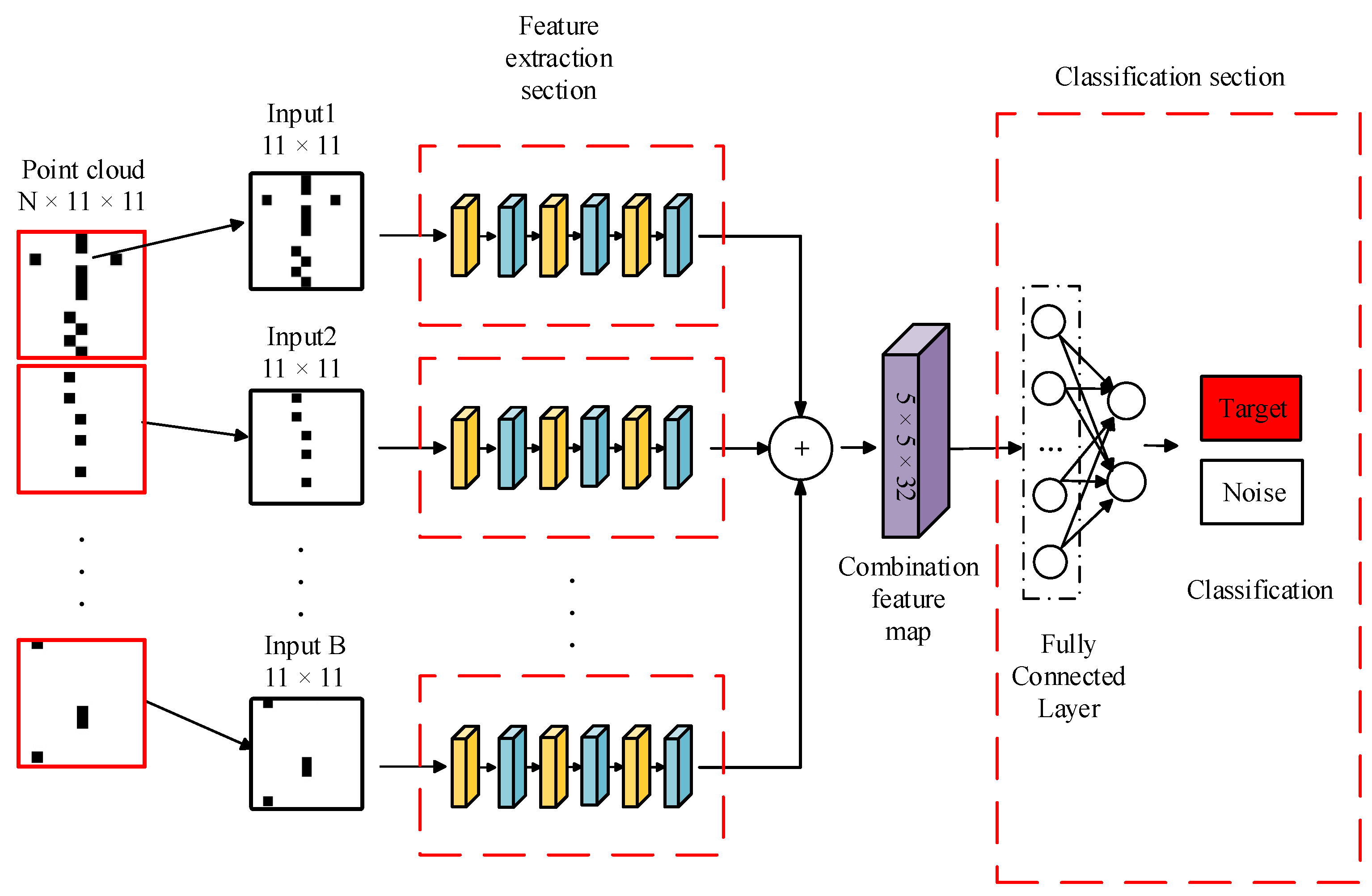
The detection performance of CNN and the CNN-PC method on the targets is analyzed through simulation experiments in this section.

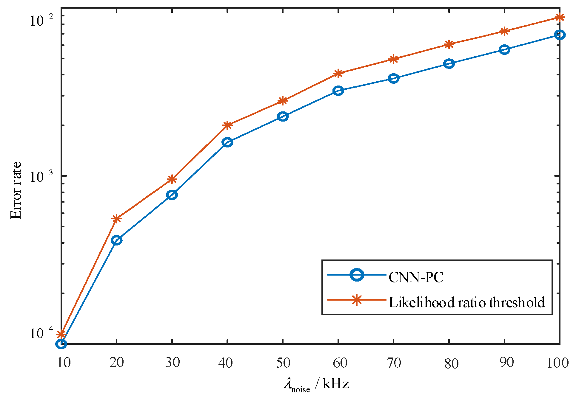
Firstly, the variation in the CNN network error rate is analyzed with respect to the noise photon rate (${\lambda }_{\mathrm{noise}}$). The error rate refers to the proportion of incorrect judgments made by CNN regarding the presence of a target in the detection bin of the detection slice. In surveillance applications, the prior probability of target existence is typically low and unknown. Hence, this experiment solely focuses on discussing the error detection proportion in CNN when no target is present in the detection bin.

Using the parameters specified in Section 5, we set the detection slice number N to be 11 and SNR to be 15dB. Under varying the noise photon rate (${\lambda }_{\mathrm{noise}}$) within the range of [10 kHz,100 kHz], a total of 60,000 detection slices are generated for each noise photon rate: 10,000 slices with pure noise and 5000 slices with target in different reference bins. The detection of these slices is performed using CNN and likelihood ratio threshold methods. Subsequently, we calculate the error rate as a function of the noise photon rate as depicted in Figure 6. The increase in the noise photon rate (${\lambda }_{\mathrm{noise}}$), as illustrated in Figure 6, leads to an upward trend in the error rates of both the CNN and likelihood ratio threshold method. However, it is worth noting that the error rate of the CNN marginally outperforms that of the likelihood ratio threshold method.

Secondly, the effectiveness of the CNN in suppressing targets within reference bins is further validated. By utilizing the parameters outlined in Section 5, we set the noise photon rate (${\lambda }_{\mathrm{noise}}$) at 50 kHz and collect 5000 detection slices with varying SNRs by adjusting the peak photon number of the pulse ($a_0$). Subsequently, the window should be slid close to the time bin where the target is located, resulting in diverse positions of the target within the region of interest and generating 5000 corresponding detection slices for each position. The region of interest pertains to a zone centered on the detection bin and encompassed by both the protection bins and reference bins. 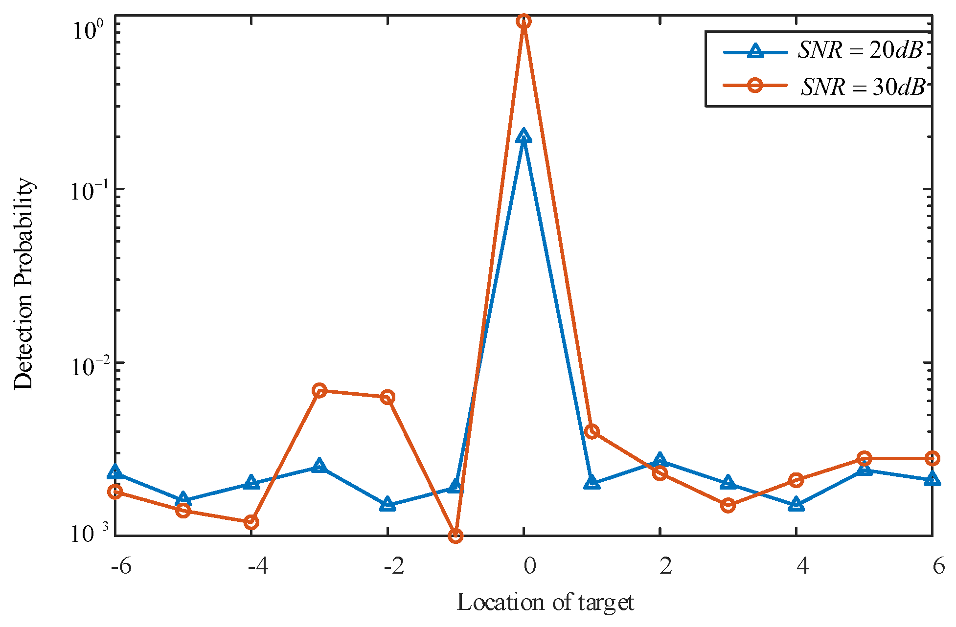The trained CNN of Section 5 is then utilized to process these slices and determine the probability of detection as illustrated in Figure 7. In Figure 7, each value on the horizontal axis represents the relative time bin number where the target is located with respect to the detection bin, with 0 indicating that the target is within the detection bin itself. This experiment also considers scenarios where the target falls into protection bins, denoted by $\pm 1$. The range from $\pm 2$ to $\pm 7$ indicates different reference bins. As depicted in Figure 7, under varying SNRs, effective target detection can only be achieved when the target resides at the detection bin; however, the probability of detecting the target is extremely low in both the reference and protection bins. This outcome aligns with the original design objective of the CNN.

The detection performance of the CNN-PC method is further analyzed by comparing it with the classical CFAR method in the following sections. The parameters mentioned in Section 5 are also utilized, with the exception that the noise photon rate (${\lambda }_{\mathrm{noise}}$) remains fixed at 50 kHz. By varying the peak photons number of the pulse ($a_0$) and the number of detection cycles (N) according to Algorithm 1, we can obtain 5000 detection slices with different SNRs.

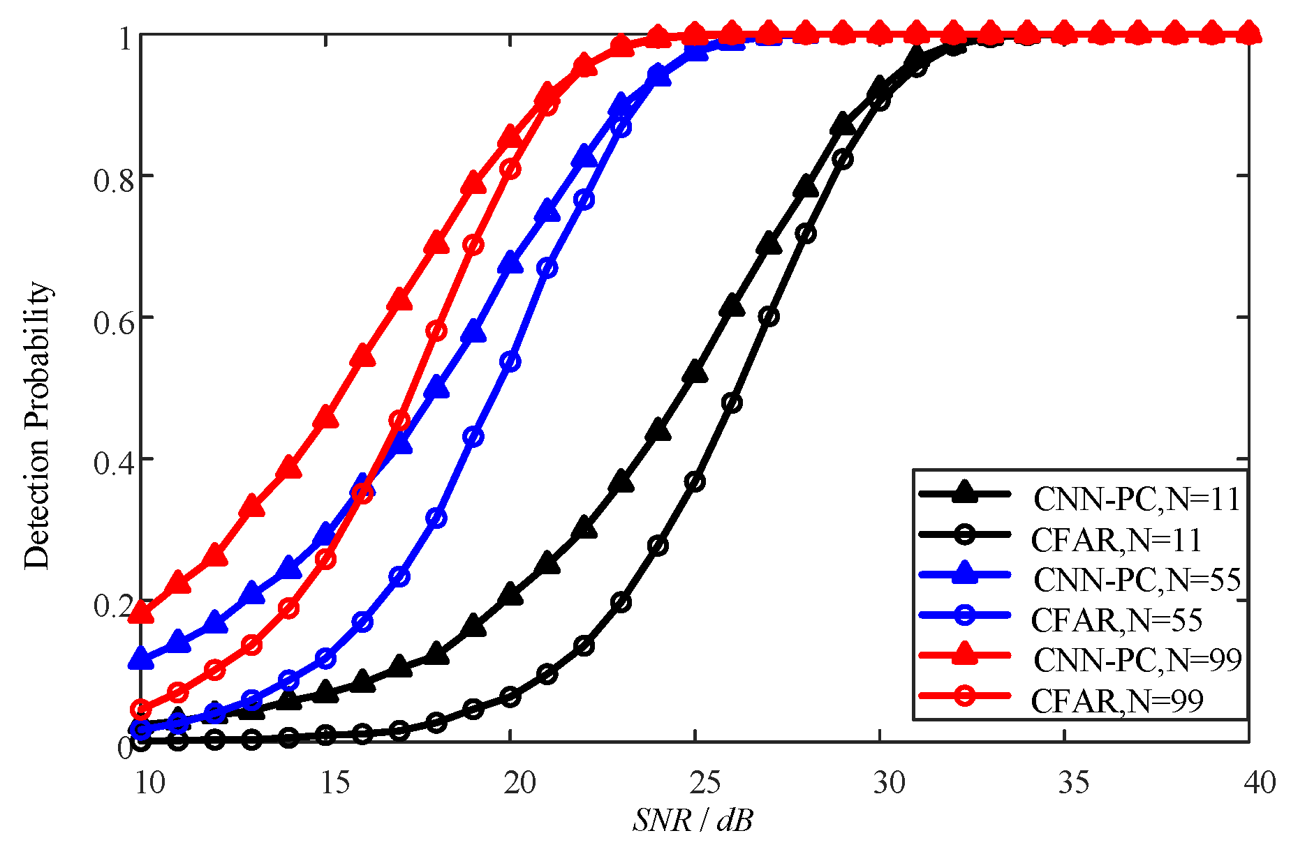
The CNN-PC method and the CFAR method, with a false alarm rate of ${10}^{-3}$, are employed for target detection, respectively. Figure 8 illustrates the corresponding detection probabilities achieved by these methods as a function of SNR and the number of detection cycles (N). As depicted in Figure 8, both the CNN-PC method and CFAR method exhibit an incremental increase in detection probability with rising SNR values. At the same SNR, the CNN-PC method has a higher detection probability. When the number of detection cycles is different, a larger number of detection cycles has superior detection performance at low SNRs. Similarly, under the same detection probability, the larger the number of detection cycles, the better the corresponding detection performance that can be achieved at a lower SNR. As the number of detection cycles increases, the corresponding improvement in the detection probability gradually slows down for both the CNN-PC and CFAR methods.

The detection performance of the CNN-PC method for the targets traversing time bins is analyzed. To demonstrate the correlation between the target echo pulse and the position within the time bin, we define the detection time difference $t_{\det }$ as the difference between the center moment of the echo pulse and that of the corresponding time bin. When $t_{\det }$ equals 0 ns, it indicates that the echo pulse coincides with its respective time bin. The parameters outlined in Section 5 are also employed, except that the noise photon rate (${\lambda }_{\mathrm{noise}}$) is set at 50 kHz and the number of detection cycles (N) is fixed at 44. By varying the peak photon number of the pulse ($a_0$), distinct detection slices with diverse SNRs for the target within the detection bin are obtained. Specifically, setting the target distance as $r_{\mathrm{t}}=2999.25\mathrm{m}$, $r_{\mathrm{t}}=3000\mathrm{m}$ and $r_{\mathrm{t}}=3000.75\mathrm{m}$ respectively yields corresponding detection time differences of $t_{\det }=-5\mathrm{ns}$, $t_{\det }=0\mathrm{ns}$ and $t_{\det }=5\mathrm{ns}$. Consequently, under each combination of detection time difference and SNR, 5000 slices are respectively generated. The CNN-PC method and CFAR method are employed for target detection. The percentage of slices in which the target is detected is computed, and the corresponding variations in detection probability with respect to SNR are illustrated in Figure 9. As depicted in Figure 9, when the target echo pulse is shifted forward relative to the detection bin (e.g., $t_{\det }=-5\mathrm{ns}$), the detection probability of the target no longer tends towards 100% as the SNR increases but rather reaches a peak at a certain level of SNR. Specifically, at 40 dB, there is a decline in the detection probability of the target. Although the CNN-PC method still outperforms the CFAR method under identical SNR conditions, both methods exhibit a rapid decrease in detection probability as SNR surpasses a specific threshold. This phenomenon indicates that it is not attributable to any algorithmic issue but rather stems from the inherent characteristics of the single-photon lidar system.

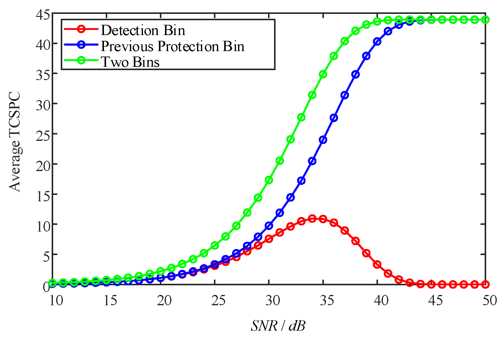
In order to analyze the cause behind the rapid decline in detection probability beyond a certain SNR threshold, when the target echo pulse is shifted forward relative to the detection bin shown in Figure 9, the average TCSPC results of the detection bin and its preceding protection bin were calculated with N = 44 and $t_{\det }=-5\mathrm{ns}$ as illustrated in Figure 10. The increase in SNR indicates an increase in the target echo energy under a certain noise level. For the target echo with $t_{\det }=-5\mathrm{ns}$, the energy in the detection bin and the protection bin in front of it are equal, implying that the average photon rate of the target is identical in both bins. As depicted in Figure 10, at lower SNRs (SNR < 25 dB), the mean TCSPC results of both cells are nearly equivalent. However, as SNR increases, there is a gradual divergence between the average TCSPC results of these two bins, with the protection bin exhibiting higher values compared to those of the detection bin. Even when SNR exceeds 35 dB, there continues to be an upward trend for the average TCSPC results in the protection bin while it is decreasing for those in the detection bin. Nevertheless, during this period, there remains an overall increasing trend when the sum of the average TCSPC results from both bins. This observation suggests that although there is a normal change trend caused by the targets’ influence on the TCSPC results, there is a reduction specifically observed within average TCSPC results from the detection bin. The average TCSPC result of the detection bin is influenced not only by the average photon rate of the target but also by the shielding effect caused by trigger events from the protection bin. When the SNR is low, the shielding effect of the protection bin may not be apparent. However, as SNR increases, there is a significant increase in the average TCSPC result of the protection bin, leading to a more prominent shielding effect on the detection bin. This subsequently affects how well the detection bin responds to trigger events and results in a decrease in the target detection probability.

Finally, the error rate introduced by the CNN-PC method is discussed. As mentioned earlier, the prior probability of the monitored target is typically very low and unknown. Therefore, the error judgment proportion of the detection slice without a target in the detection bin can approximately represent the error rate of the CNN-PC method. By utilizing the parameters specified in Section 5, we set the noise photon rate (${\lambda }_{\mathrm{noise}}$) to 50 kHz and maintain a SNR of 15 dB. Under a different number of detection cycles (N), we generated 10,000 detection slices consisting solely of pure noise and simultaneously produced 5000 detection slices with targets in different reference bins. This allowed us to obtain a total of 60,000 detection slices under a varying number of detection cycles (N). Both the CNN-PC method and likelihood ratio threshold method were employed for detecting these slices, and statistical analysis was conducted on each method’s error rate as N changed. The results are illustrated in Figure 11. As can be seen from Figure 11, the error rates of both methods increase in tandem as the number of detection cycles (N) increases. Over time, the error rates of both methods gradually converge towards equality. Despite the increasing error rate with a higher number of detection cycles (N), it remains consistently low and has minimal impact on the performance of the lidar system.

7.2. Experimental Results

The actual data collected by single-photon lidar are utilized in this section to validate the detection performance of the CNN-PC method. In the experiment, a $64\times 64$ Gm-APD array with a parabolic laser pulse at a pulse repetition frequency of 20 kHz and laser pulse duration of ${\tau }_{\mathrm{w}}=20\mathrm{ns}$, as well as time bin width of ${\tau }_{\mathrm{s}}=20\mathrm{ns}$, is employed for the single-photon lidar. The single-photon lidar employs a single beam of floodlight to effectively detect the power line tower target located approximately $450\mathrm{m}$ above it, operating in a fixed gaze mode. 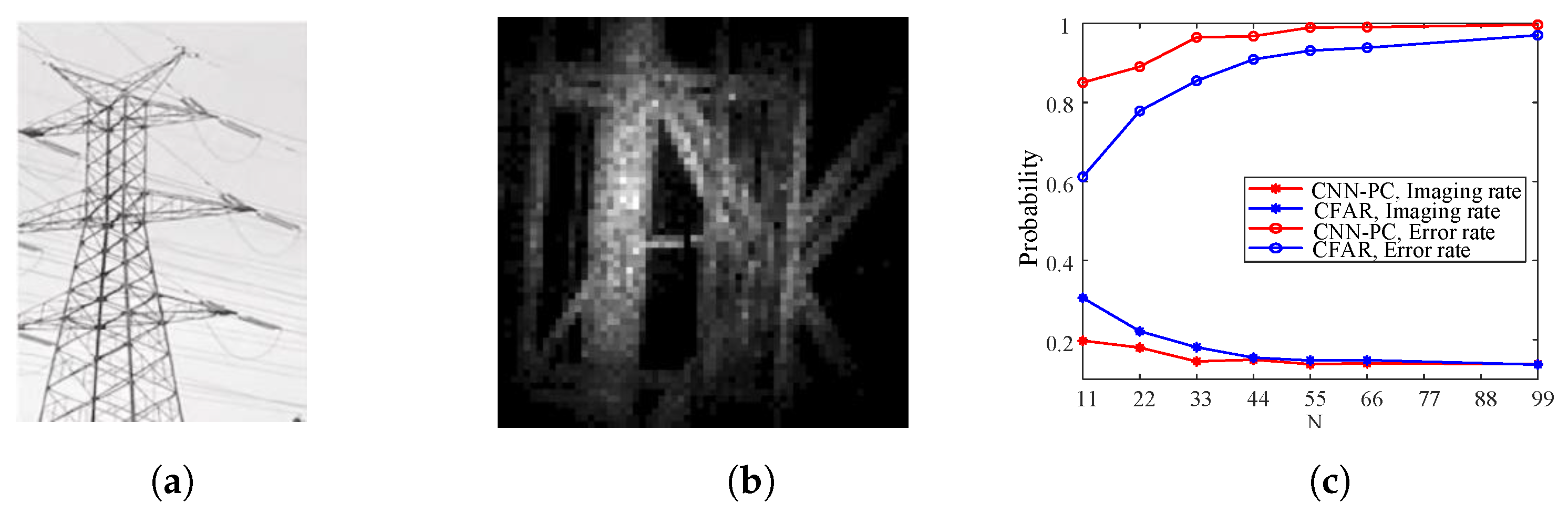Figure 12a illustrates the optical image of the detected target, while Figure 12b presents results obtained using a fixed threshold of 50 based on the TCSPC results from 1980 detection cycles. According to the imaging results in Figure 12b, the average TCSPC result corresponding to pixels without detected targets is considered as the noise intensity. Additionally, the TCSPC result corresponding to the brightest pixel in Figure 12b is taken as the maximum intensity of the target, while the fixed threshold is regarded as the minimum intensity of the target. It can be estimated that the experimental SNR varies within a range of $[2.45\mathrm{dB},17.96\mathrm{dB}]$.

The CNN-PC method’s detection performance is evaluated at different numbers of detection cycles by considering the pixels shown in Figure 12b as valid pixels. The imaging rate $r_{\mathrm{image}}$ is then defined as the ratio of valid pixel points in the imaging result to the total number of valid pixels in Figure 12b. In this experiment, the CNN-PC method’s detection performance is analyzed using actual data imaging results. Therefore, the corresponding error rate can be described as the proportion of error detection pixels in the entire image pixel for the CNN-PC method. Error detection pixels refer to points where the imaging results have different validity descriptions compared to their corresponding pixels in Figure 12b. The imaging rates and error rates of both the CNN-PC method and CFAR method vary with the number of detection cycles as depicted in Figure 12c; it should be noted that the false alarm rate for the CFAR method remains at a constant value of ${10}^{-3}$.

The CNN-PC method exhibits an imaging rate of approximately $85\%$ when N = 11, as depicted in Figure 12c, which is significantly higher than that achieved by the CFAR method. Moreover, the error rate of the CNN-PC method at this point stands at around 20%, which is notably lower than that of the CFAR method. As the number of detection cycles increases, both methods demonstrate a corresponding increase in the imaging rate and a gradual decrease in the error rate. Consequently, the disparity between their respective imaging rates and error rates diminishes. Notably, the CNN-PC method achieves near-perfect imaging rates with an error rate of approximately 13% when the number of detection cycles exceeds 55. Similarly, for N = 99, the CFAR method attains an imaging rate around 95% while maintaining an error rate of about 13%. Evidently, at equivalent numbers of detection cycles, the CNN-PC method outperforms with its superior imaging rate and reduced error rate. Additionally, the CNN-PC method requires fewer detection cycles at same level of imaging rate or error rate. Consequently, it proves more suitable for scenarios where limitations exist on the number of detection cycles.

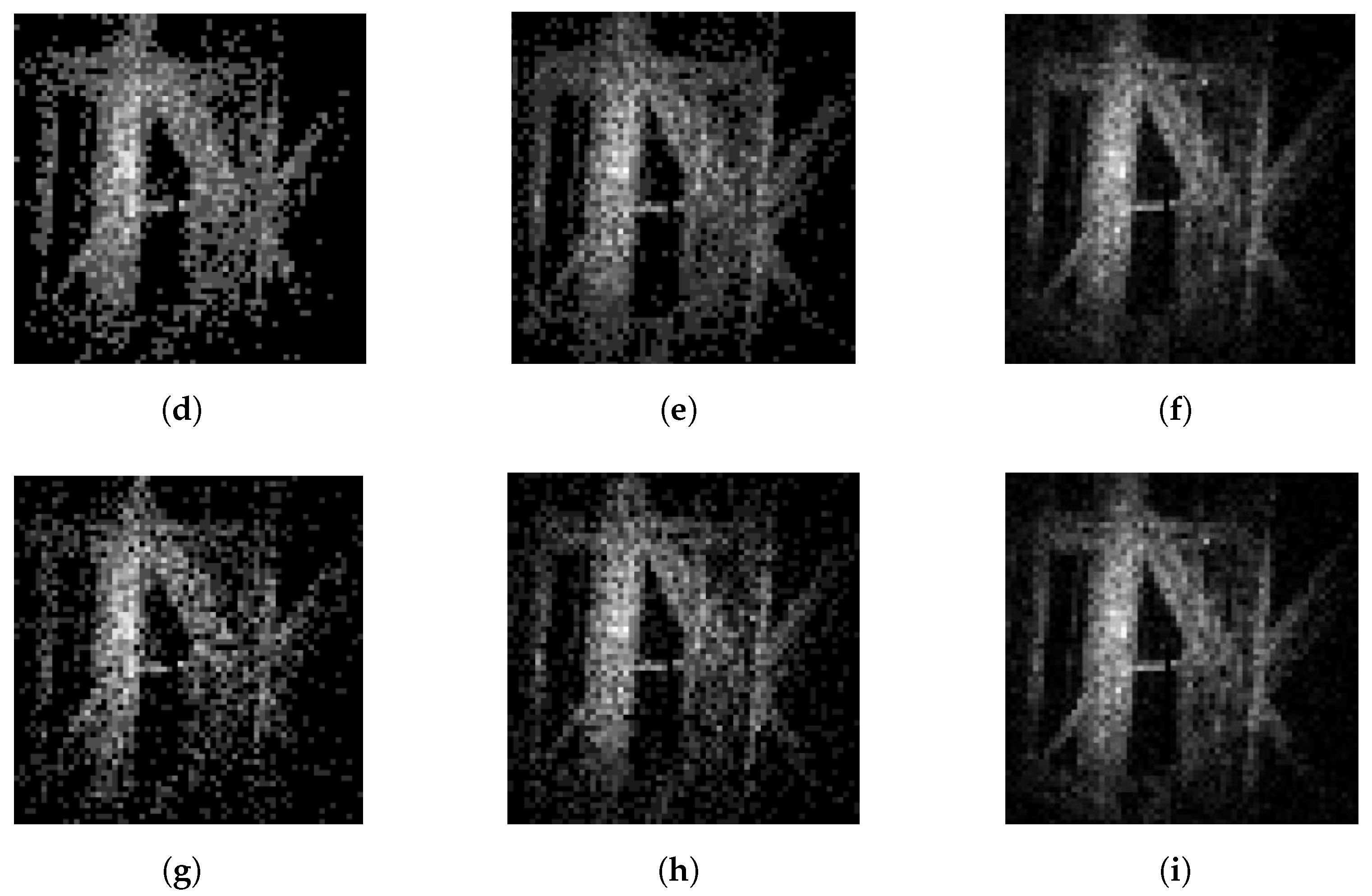
The imaging results are presented in Figure 12d–i for $N=11$, $N=22$, and $N=99$ using the CNN-PC method and CFAR method. Comparing Figure 12d–f, it is evident that increasing the number of detection cycles leads to the CNN-PC method capturing more effective pixels in the target image, resulting in a smoother and clearer image. Similar conclusions can be drawn from the corresponding imaging results of the CFAR method shown in Figure 12g–i. A comparison between Figure 12d,g reveals that when $N=11$, the CNN-PC method detects more pixel points than the CFAR method. As observed in Figure 12f,i, at $N=99$, the CNN-PC method significantly improves the imaging quality compared to the CFAR method; however, their difference becomes less pronounced. Therefore, under a small number of detection cycles, the CNN-PC method exhibits greater advantages.

8. Discussion

The single-photon lidar system must minimize the number of detection cycles in order to effectively monitor large areas with a high refresh rate. In this study, instead of utilizing the accumulated TCSPC results values from multiple detection cycles for target detection, we directly form 2D detection slices through multiple detection cycles and achieve target detection based on these slices. The proposed CNN-PC method leverages CNN to extract features from the detection slices and comprehensively processes the features of multiple slices for target identification and classification. This approach exhibits low sensitivity to the number of detection cycles while demonstrating a robust capability in detecting weak targets.

Compared to TCSPC, 2D detection slices provide an intuitive characterization of point cloud features without any loss of information after dimensionality reduction. Consequently, processing directly on these detection slices enables the extraction of more effective features, leading to the superior performance of the CNN-PC method in target detection compared to the TCSPC-based detection method [9,10,11]. Furthermore, when compared to threshold-based methods [5,6,7], the CNN-PC method exhibits improved error rates and detection probabilities. Notably, as the target echo pulse is shifted forward relative to the detection bin, there is a rapid decrease in the detection probability once the SNR surpasses a certain threshold. This phenomenon can be attributed to the shielding effect caused by trigger events from protection bin preceding the detection bin. It is important to note that this inherent characteristic of single-photon lidar has no bearing on the target detection methodology.

However, it is important to acknowledge the potential challenges and limitations associated with CNN-PC. The CNN-PC method is constrained by the restriction of allowing only one target in the detection slice. Consequently, this limitation results in small available detection slices, posing difficulties for feature mining. Furthermore, when processing multiple detection slices, each slice is adjacent to one another without any overlap, which also imposes a constraint on the selection of the number of detection cycles.

9. Conclusions

In this paper, CNN is introduced for feature extraction from 2D point cloud slices, and based on this, the CNN-PC method is proposed for target detection in single-photon lidar. The method enables target detection with fewer detection cycles, facilitating the application of single-photon lidar in large-scale surveillance scenarios with high refresh rates. Additionally, the CNN-PC method exhibits a robust capability to detect weak targets.

Compared to the traditional target detection method of single-photon lidar, the CNN-PC method exhibits evident advantages in terms of the target detection performance, error rate, and imaging rate. However, a limitation of the CNN-PC method lies in its utilization of excessively small detection slices, which somewhat impacts its overall performance. Therefore, further research is needed to explore breakthroughs in overcoming this size constraint on detection slices. Additionally, it is essential to investigate improvements in the detection scheme when dealing with overlapping multiple detection slices.

References

1. Hadfield, R.H. Single-photon detectors for optical quantum information applications. Nat. Photonics 2009, 3, 696–705. [Google Scholar] [CrossRef]
2. Tan, C.S.; Kong, W.; Huang, G.H.; Hou, J. Long-Range Daytime 3D Imaging Lidar With Short Acquisition Time Based on 64 × 64 Gm-APD Array. Photonics J. 2022, 3, 6623407. [Google Scholar] [CrossRef]
3. Wu, C.; Xing, W.G.; Xia, L.H.; Huang, H.X. Improvement of detection performance on single-photon lidar by EMD-based denoising method. Optik 2019, 181, 760–767. [Google Scholar] [CrossRef]
4. Wang, M.Q.; Sun, J.F.; Li, S.N.; Lu, W.; Zhou, X.; Zhang, H.L. A photon-number-based systematic algorithm for range image recovery of GM-APD lidar under few-frames detection. Infrared Phys. Technol. 2022, 125, 104267. [Google Scholar] [CrossRef]
5. Xu, L. Improving on Detection Performance of Pulse Accumulated Gm-APD Lidar. Ph.D. Thesis, Harbin Institute of Technology, Harbin, China, 2017. [Google Scholar]
6. Jiang, Z.M.; Gong, C.; Xu, Z.Y. Varied threshold with laser flight time in scannerless range-gated ladar. IEEE Trans. Wirel. Commun. 2019, 18, 6015–6029. [Google Scholar] [CrossRef]
7. Chen, Z.; Liu, B.; Guo, G.M. Adaptive single photon detection under fluctuating background noise. Opt. Express 2020, 28, 30199–30209. [Google Scholar] [CrossRef] [PubMed]
8. Liu, Z.W.; Li, Z.Q.; Su, Z.G. Detection of Constant False Alarms Based on Single-photon lidar. Chin. J. Lasers 2023, 50, 184–192. [Google Scholar] [CrossRef]
9. Hu, S.J.; He, Y.; Yuan, J.Y.; Lv, D.L.; Hou, C.H.; Chen, W.B. Method for Solving Echo Time of Pulse Laser Ranging Based on Deep Learning. Chin. J. Lasers 2019, 46, 302–311. [Google Scholar] [CrossRef]
10. Bai, Y.B.; Pan, K.L.; Geng, L. Signal Processing of Spatial Convolutional Neural Network for Laser Ranging. Chin. J. Lasers 2021, 48, 38–48. [Google Scholar] [CrossRef]
11. Chen, G.B.; Landmeyer, F.; Wiede, C.; Kokozinski, R. Feature extraction and neural network-based multi-peak analysis on time-correlated LiDAR histograms. J. Opt. 2022, 24, 034008. [Google Scholar] [CrossRef]
12. Johnson, S.E. Target detection with randomized thresholds for lidar applications. Appl. Opt. 2012, 51, 4139–4150. [Google Scholar] [CrossRef] [PubMed]
13. Wu, S.; Wang, G.R.; Tang, P.; Chen, F.; Shi, L.P. Convolution with even-sized kernels and symmetric padding. In Proceedings of the Advances in Neural Information Processing Systems 32 (NeurIPS), Vancouver, BC, Canada, 8–14 December 2019; pp. 1192–1203. [Google Scholar]
14. Szegedy, C.; Wanhoucke, V.; Ioffe, S.; Shlens, J.; Wojna, Z. Rethinking the Inception Architecture for Computer Vision. In Proceedings of the 2016 IEEE Conference on Computer Vision and Pattern Recognition (CVPR), Las Vegas, NV, USA, 27–30 June 2016; pp. 2818–2826. [Google Scholar]
Figure 1. A 2D point cloud map with multiple detection cycles.
Photonics 11 00043 g001
Figure 2. Detection slices of 2D point cloud. (a) Target present within the detection bin; (b) no target in the detection slice; (c) target present within the reference bin.
Photonics 11 00043 g002
Figure 3. Structure of CNN.
Photonics 11 00043 g003
Figure 4. Accuracy and loss curves during CNN training process.
Photonics 11 00043 g004
Figure 5. CNN-PC method.
Photonics 11 00043 g005
Figure 6. The variation of error rates with noise photon rate ( λ noise ).
Photonics 11 00043 g006
Figure 7. The probability of targets in different locations of the detection slice being detected by the CNN.
Photonics 11 00043 g007
Figure 8. The variation of detection probability with SNR for the CNN-PC method and CFAR method.
Photonics 11 00043 g008
Figure 9. The variation of detection probability with SNR for the CNN-PC method and CFAR method under different t det .
Photonics 11 00043 g009
Figure 10. The variation of average TCSPC result with SNR at t det = 5 ns.
Photonics 11 00043 g010
Figure 11. The variation of error rates as the number of detection cycles (N) changed.
Photonics 11 00043 g011
Figure 12. The imaging results obtained using Gm-APD array. (a) The optical image of the observed target; (b) Imaging result achieved with N = 1980 ; (c) The variations of imaging rate and error rate; (d) Imaging result obtained using CNN-PC method for N = 11 ; (e) Imaging result obtained using CNN-PC method for N = 22 ; (f) Imaging result obtained using CNN-PC method for N = 99 ; (g) Imaging result obtained using CFAR method for N = 11 ; (h) Imaging result obtained using CFAR method for N = 22 ; (i) Imaging result obtained using CFAR method for N = 99 .
Photonics 11 00043 g012aPhotonics 11 00043 g012b