Abstract
Different from the radio frequency bipolar complex signalling, LED-based visible light communication (LED-VLC) meets the non-negativity requirement by adding a bias component (BC) to a bipolar real-valued signal. Although many people know that there is a relationship between BC and LED characteristics, unfortunately, most of them chose to ignore it, and thus there has been little exploration of its impact on VLC. In this paper, we have experimentally measured the frequency domain characteristics of several LEDs commonly used in home and business applications. The numerical calculations show that the logarithmic domain absolute frequency response is approximately linear, where the corresponding intercepts and slopes can be quadratically expressed with respect to BC with a very low fitting error. This experimental investigation reveals that the BC value will remarkably influence the VLC system performance beyond non-negativity, and the LED-VLC transceiver designs should jointly take the BC and LED communication characteristic into consideration.
1. Introduction
As a special sub-domain of wireless communications, visible light communication utilizes off-the-shelf light-emitting diodes (LED) as transmitters to emit the signals and simultaneously provide satisfactory illumination [1], where t is the time instance and is the bias voltage. Since the input of LED is required to be non-negative real-valued (NRV), , the bipolar signal component is generally added by a bias component (BC) using Bias-Tee equipment. Therefore, the main difference between antenna-based radio-frequency (RF) and VLC is that the input of RF antenna, , can be bipolar complex-valued. At the receiver side, the noise-free received signal of VLC can be expressed as , where is the additive channel noise and is the equivalent channel impulse response closely related to the channel bandwidth.
To improve the transmission rate of VLC, there are numerical approaches such as high-order modulation format [2], blue light filtering [3], pre-equalization [4], post-equalization [5], discrete multitone modulation (DMT) [6,7], optical MIMO [8] and micro-LED array [9,10]. These schemes focus on the energy-efficient designs of [2,6,7,8], or improving the time-domain or frequency domain performance of [3,4,5]. For these works, two fundamental assumptions for VLC system designs are the NRV assumption and that the value of BC, , will not influence other key performance indicators of VLC, such as the 3 dB bandwidth of . We notice that the author of [11] mainly selects the bias according to the indoor lighting standard, without in-depth analysis of the impact of bias on frequency response and modulation bandwidth. The authors of [10] have designed complementary metal oxide semiconductor (CMOS)-controlled micro-LEDs and experimentally demonstrated that will remarkably influence with respect to the available modulation bandwidth, which is up to 185 MHz for these LEDs specially designed for VLC. This important fact implies that when we design for CMOS-controlled micro-LEDs, we should jointly consider and , whose frequency domain transformation is defined by . Furthermore, the authors of [10] also pointed out that , the frequency domain of , satisfies
where represents the carrier lifetime within the device active region. With the increase in the bias current or , the carrier concentration in the PN junction increases, becomes smaller and thus, will increase. Unfortunately, the authors [10] failed to develop a general numerical model of the relationship between and for CMOS-controlled LED. In addition, this model is not necessarily applicable to commercially available LEDs. Compared with specially designed LEDs, it will be more meaningful to establish a specific numerical relationship model between and for commercially available LEDs. The reasons mainly include the following two aspects: first, commercially available LEDs are the basis for transforming into access points and communication base stations of ordinary end networks, integrating communication and lighting, and upgrading from green lighting to smart lighting. Secondly, the 3 dB bandwidth of commercially available LED is only a few MHZ, which is the bottleneck restricting the rapid development of visible light communication. By establishing the specific numerical model of and , we can not only understand the specific influence of on , but also combine the model to balance the LED to broaden its available bandwidth, so as to optimize the VLC system.
Motivated by the aforementioned considerations, we conducted experiments on several representative commercially available LEDs, modelling with respect to . We demonstrate that can be well approximated by a log-domain linear function of with a very low fitting error; say, . Furthermore, we show that the intercept and slope of the low-domain line, and , can be described by first or quadratic functions with respect to . These are the first experimental results to characterize how the bias setup influences the frequency domain characteristics of commercially available LED. These results also provide more insight into the joint consideration of bias setup and transceiver designs and indicate that the bias setup imposes constraints more than NRV on the VLC system compared with its antenna-based RF counterpart.
2. Theoretical Analysis
In this section, we mainly introduce how the affects the amplitude–frequency response of the LED.
The LED equivalent circuit is shown in Figure 1 [12]. The parallel network composed of and C shows the junction resistance and junction capacitance of the PN junction in the LED. and L are the cascade resistance and parasitic inductance of the metal pin connection at both ends of the LED and the surface of the coating layer, respectively, which are the main factors leading to LED heating. The LED emits photons through the PN junction. The structure of the PN junction directly affects the luminescence characteristics of the LED. The carrier lifetime —that is, the average recombination time of electrons and holes—affects the frequency response of the LED. The domain equivalent impedance of LED is:
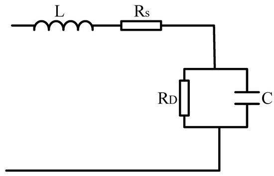
Figure 1.
The LED equivalent circuit.
It can be seen from Equation (2) that when f is fixed, the or bias current becomes larger, becomes smaller, and the role of and C is enhanced. When the input signal power is constant, the power divided by and C will become larger. In essence, this shows that or bias current affects the amplitude–frequency response of LED. Similarly, when is fixed, with the increase of f, the effect of and C is weakened, and the energy is mainly distributed in the form of thermal energy, which is also the reason why the LED frequency response gradually decreases with the increase in frequency.
3. Experimental System
In this paper, our primary task is to experimentally characterize the influence of the LED bias on the frequency domain channel response . To this end, in this section, we present the system setup and the corresponding measurement approach.
3.1. System Setup
The experimental system diagram and setup are illustrated by Figure 2 and Figure 3, respectively. The system in Figure 3 consists of the following blocks: signal source, bias setup, LED transmitter, photodiode (PD) receiver, and vector network analyser (VNA). The signal source is the ZNB20 vector network analyser produced by Rhode & Schwartz. The VNA can produce bipolar signals, , from 100 KHz to 20 GHz. The bias voltage, , is provided by a multi-channel linear DC voltage source, GPS-3303C. The PD is S10784 silicon photodiode. The Bias-T, ZFBT-4R2GW+, has a passband of 0.1–4200 MHz and can generate , such that the input for LED is VNA, . The output of PD, , is fed back to VNA. Then, comparing and , the frequency domain channel response can be estimated. Since the bandwidths of PD and Bias-T are much larger compared with that of LED, the estimated mainly relies on and can be approximated as the frequency domain characteristic of LED.
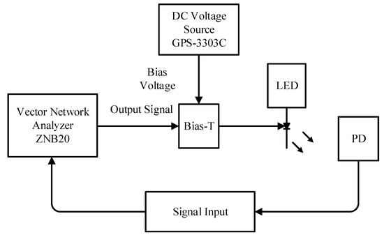
Figure 2.
Experimental schematic diagram.
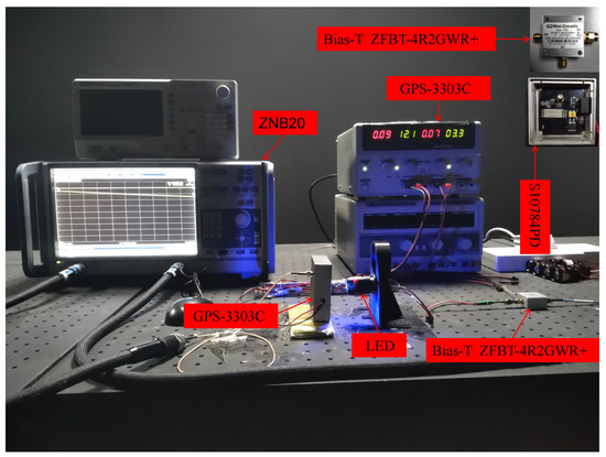
Figure 3.
Real experimental environment.
3.2. Measuring Approach
3.2.1. LEDs to Be Measured
Commercially available LEDs are mainly divided into white LED and monochrome LED. White LED mainly has two categories: PC-LED and RGB-LED. The PC-LED is coated with yellow phosphor on the outside of blue LED (B-LED). Through appropriate design, a part of blue light is emitted through the phosphor coating to form the blue part of the spectrum. At the same time, the phosphor converts the remaining part of blue light into the red and green parts of the spectrum, thus generating white light. RGB-LED produces white light by mixing red LED (R-LED), green LED (G-LED) and blue LED, packaging the three colours together and adjusting the power of each colour LED. Compared with RGB-LED, PC-LED is more common in the commercial field because of its cheap price and simple structure. The main monochrome LED includes red LED, green LED and blue LED. In this paper, we measure for the SMD PC-LED of Model 5730 (5.7 mm × 3.0 mm) with rated power of 0.5 W and monochrome LED (including R-LED, G-LED and B-LED) of SMD 2835 (2.8 mm × 3.5 mm) with rated power of 0.5 W. The LED we measured here refers to LED lamp beads. At present, most of the LED lights used in homes and businesses are welded by these several types of LED lamp beads, so the LED lamp beads we choose are representative. In previous measurements, we have found that the frequency response of monochrome LED was similar. In order to make the paper more concise, we only analysed PC-LED and B-LED in detail. Figure A1 and Figure A2 are amplitude-frequency response and fitting straight lines of R-LED and G-LED, which are given in the Appendix A of the paper and will not be analyzed in detail.
3.2.2. Measuring Range
To fix the system setup, the bias voltage of LED is gradually increased to examine the influence of bias voltage on the amplitude–frequency characteristic response of LED. In order to fully explore the influence of bias voltage on the amplitude-frequency characteristics of LED, and to ensure that the LED will not burn out due to excessive power, we choose a bias voltage range of 3.0∼4.2 V. When the bias voltage is 4.2 V, the power of the LED is nearly twice the rated power. Therefore, the bias component should be smaller than 4.2 V. LED has a 3 dB modulation bandwidth up to several MHz for most of the commercially available LEDs. The PC-LED is lower due to the influence of phosphor. We focus on the frequency range of PC-LED and B-LED for 1–10 MHz and 1–20 MHz, respectively.
3.2.3. Measuring Procedure
During measuring processing, the VNA ZNB20 uniformly samples 201 points of the selected frequency range under a single bias voltage. In order to facilitate modelling and analysis of bias voltage and amplitude–frequency response, in the experiment, we use to represent the frequency response in dB, f to represent the frequency in MHz, and to represent the bias voltage in V.
4. Experimental Results and Analysis
Using the experimental system setup in Section 3, we will measure the LED spectral characteristics and analyse the fitting error to show the reasonability of the proposed model in this section.
4.1. Experimental Results and Fitting Analysis
4.1.1. Error Function of Proposed Model
To show the reasonability of the proposed log-linear model, we first present the processing error definition. To analyse the fitting error between the measured data and the proposed model, we resort to MATLAB 2021a, where the fitting error defined by R-squared (Coefficient of Determination) is given by
where is the experimental measured data, is the predicted value based on the proposed fitting equation, and is the average value of the measured value. Here, R-squared ranges from zero to one and a larger R-squared value implies a more precise proposed model.
4.1.2. Polynomial Order Determination in Log-Domain
In this paper, we use a log-domain polynomial to fit the measured data. To show our main motivation, we first recall the proposed model in (1) for special-purpose LED of VLC in (1). With the increase in the bias current, the carrier life in (1) will become smaller and result in a polynomial negative slope of . We use this model to fit the measured data and show the comparison in Figure 4. As illustrated by Figure 4, when the bias voltage is 3.0 V, R-Squared is 0.113, and when the bias voltage is 4.2 V, R-Squared is 0.065. Consequently, the existing model in (1) is not applicable to the commercially available LEDs. For this reason, we propose to fit the measured data using a log-domain polynomial. For this purpose, we first determine the polynomial order of in the log-domain for two kinds of LEDs under different . R-squared obtained from linear fitting and quadratic curve fitting is shown in Figure 5, which illustrates that the R-square values of these two fitting schemes approach one for different , implying linear fitting is sufficient. In addition, higher-order polynomial fitting also increases the processing complexity. Therefore, in the following discussion, we focus on the log-domain linear model analysis.
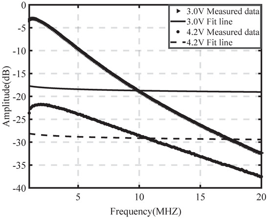
Figure 4.
Model (1) in [10] and the measured data of B-LED.
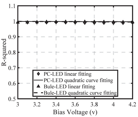
Figure 5.
R-squared for linear and quadratic fitting of amplitude–frequency response of two LEDs at different bias voltages.
4.1.3. Proposed Log-Domain Linear Model and Fitting Error
Now, we present the proposed log-domain linear model and analyse the fitting error. We formally introduce the log-domain linear model below
where S represents the slope of the fitting straight line under different bias voltages, while I is the intercept of the fitting straight line under different bias voltages and represents the frequency response value predicted according to the fitting straight line when the frequency is 0 MHz. The amplitude-frequency responses measured at different bias voltages and the log-domain linear fitting results are given by Figure 6 and Figure 7. The expressions of the fitted lines are listed in Table 1 and Table 2. For these proposed models, the fitting error with respect to R-squared value is shown in Figure 8, from which we can see that the minimum value of R-squared for two kinds of LED is 0.988.
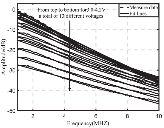
Figure 6.
PC-LED amplitude–frequency response and fitting straight lines.
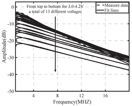
Figure 7.
B-LED amplitude–frequency response and fitting straight lines.

Table 1.
Linear Fitting Equations for PC-LED at Different Bias Voltages.
Table 2.
Linear Fitting Equations for Bule-LED at Different Bias Voltages.
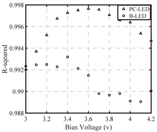
Figure 8.
Linear fitting R-squared for two LEDs with different bias voltages.
Next, we investigate the relationship between and S or I. Figure 6 and Figure 7 are the fitting lines of the two LEDs under different voltages. The points in Figure 9 are the slopes of the fitting lines under different bias voltages of the two LEDs. The points in Figure 10 are the intercepts of the fitting lines under different bias voltages of the two LEDs; that is, the value of the intersection of the fitting line and the X-axis. Using the MATLAB 2021a fitting tool to fit the points in Figure 9 and Figure 10 with the minimum error, the fitting lines in Figure 9 and Figure 10 are obtained, and the corresponding expressions of PC-LED and B-LED are obtained as follows:
where is the slope of the PC-LED fitting straight line and is the slope of the B-LED fitting straight-line.
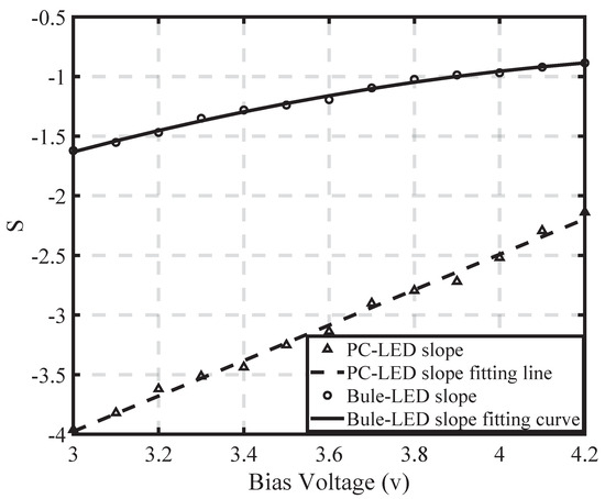
Figure 9.
Slope and fitting curves of two LEDs with different bias voltages.
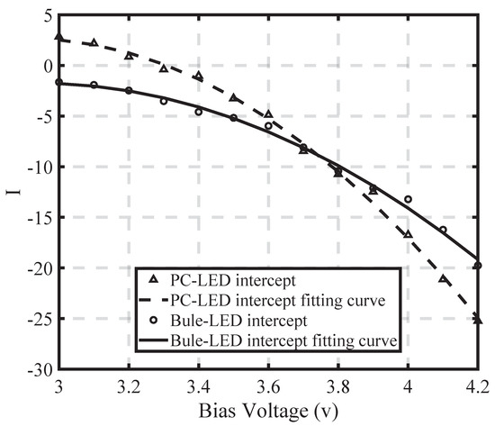
Figure 10.
Intercept and fitting curves of two LEDs with different bias voltages.
By substituting Equations (5) and (7) into Equation (4), the PC-LED bias voltage and amplitude–frequency response model can be obtained, as shown by (9).
By using similar techniques, for B-LED, we get (10).
So far, we have established a log-domain linear model of relative to f, which is the first model to establish the specific relationship between , f and of commercially used LEDs through experiments. From the model we can see that for fixed f, relative to the is a second-order polynomial function. The same applies for fixed LED at low frequency: and f is approximately linear correlation. This model can directly guide us to consider to balance the LED, broaden the available bandwidth of the LED, and design the optimal VLC system.
5. Conclusions
In this paper, we have experimentally investigated the spectral characteristics of commercially available LEDs and revealed that the equivalent spectral function can be well approximated by a log-domain function with respect to f. Our main findings indicate that (1) the traditional model of LED specialized for VLC is not applicable to the commercially available LEDs; (2) the bias setup can remarkably influence the system bandwidth and thus should be taken into consideration for VLC system design beyond satisfying the non-negativity requirement. We believe that the more deeply we investigate the LED characteristics in relation to the performance of the VLC system, the more unique potential technologies of VLC will be dug out in future research.
Author Contributions
Conceptualization, L.L. and Y.Z.; Methodology, B.B.; Resources, L.L.; Data curation, L.L.; Visualization, Y.Z. and L.L.; Supervision, T.Y. All authors have read and agreed to the published version of the manuscript.
Funding
This research received no external funding.
Institutional Review Board Statement
Not applicable.
Informed Consent Statement
Not applicable.
Data Availability Statement
The data used to support the findings of this study are available from the corresponding author upon request.
Acknowledgments
The authors would like to acknowledge the support of the tutor and the collaboration efforts of colleagues.
Conflicts of Interest
The authors declare no conflict of interest.
Abbreviations
The following abbreviations are used in this manuscript:
| VLC | Visible light communication. |
| LED | Light emitting diode. |
| NRV | Nonnegative real-valued. |
| BC | Bias component. |
| RF | Radio frequency. |
| DMT | Discrete multitone modulation. |
| CMOS | Complementary metal oxide semiconductor. |
| VNA | Vector network analyser. |
| PD | Photodiode |
Appendix A

Figure A1.
G-LED amplitude-frequency response and fitting straight lines.
Figure A1.
G-LED amplitude-frequency response and fitting straight lines.


Figure A2.
R-LED amplitude-frequency response and fitting straight lines.
Figure A2.
R-LED amplitude-frequency response and fitting straight lines.

References
- Bao, X.; Yu, G.; Dai, J.; Zhu, X. Li-Fi: Light fidelity-a survey. Wireless Netw. 2015, 21, 1879–1889. [Google Scholar] [CrossRef]
- Langer, K.D.; Vučić, J.; Kottke, C.; Fernández, L.; Habe, K.; Paraskevopoulos, A.; Wendl, M.; Markov, V. Exploring the potentials of optical-wireless communication using white LEDs. In Proceedings of the 2011 13th International Conference on Transparent Optical Networks, Stockholm, Sweden, 26–30 June 2011; IEEE: Piscataway, NJ, USA, 2011; pp. 1–5. [Google Scholar]
- Grubor, J.; Lee, S.C.J.; Langer, K.D.; Koonen, T.; Walewski, J.W. Wireless high-speed data transmission with phosphorescent white-light LEDs. In Proceedings of the 33rd European Conference and Exhibition of Optical Communication-Post-Deadline Papers (Published 2008), Berlin, Germany, 16–20 September 2007; VDE: Frankfurt am Main, Germay, 2007; pp. 1–2. [Google Scholar]
- Le Minh, H.; O’Brien, D.; Faulkner, G.; Zeng, L.; Lee, K.; Jung, D.; Oh, Y. High-Speed Visible Light Communications Using Multiple-Resonant Equalization. IEEE Photonics Technol. Lett. 2008, 20, 1243–1245. [Google Scholar] [CrossRef]
- Le Minh, H.; O’Brien, D.; Faulkner, G.; Zeng, L.; Lee, K.; Jung, D.; Oh, Y.; Won, E.T. 100-Mb/s NRZ Visible Light Communications Using a Postequalized White LED. IEEE Photonics Technol. Lett. 2009, 21, 1063–1065. [Google Scholar] [CrossRef]
- Vučić, J.; Kottke, C.; Nerreter, S.; Langer, K.D.; Walewski, J.W. 513 Mbit/s visible light communications link based on DMT-modulation of a white LED. J. Light. Technol. 2010, 28, 3512–3518. [Google Scholar] [CrossRef]
- Khalid, A.M.; Cossu, G.; Corsini, R.; Choudhury, P.; Ciaramella, E. 1-Gb/s transmission over a phosphorescent white LED by using rate-adaptive discrete multitone modulation. IEEE Photonics J. 2012, 4, 1465–1473. [Google Scholar] [CrossRef]
- Azhar, A.H.; Tran, T.A.; O’Brien, D. Demonstration of high-speed data transmission using MIMO-OFDM visible light communications. In Proceedings of the 2010 IEEE Globecom Workshops, Miami, FL, USA, 6–10 December 2010; IEEE: Piscataway, NJ, USA, 2010; pp. 1052–1056. [Google Scholar]
- Zhao, C.; Li, W.; Yan, G.; Liu, Z. Application of Micro-LED in Visible Light Communication. In SID Symposium Digest of Technical Papers; Wiley: Hoboken, NJ, USA, 2020; Volume 51, pp. 117–120. [Google Scholar]
- McKendry, J.J.D.; Massoubre, D.; Zhang, S.; Rae, B.R.; Green, R.P.; Gu, E.; Henderson, R.K.; Kelly, A.E.; Dawson, M.D. Visible-light communications using a CMOS-controlled micro-light-emitting-diode array. J. Light. Technol. 2012, 30, 61–67. [Google Scholar] [CrossRef]
- Chun, H.; Manousiadis, P.; Rajbhandari, S.; Vithanage, D.A.; Faulkner, G.; Tsonev, D.; McKendry, J.J.D.; Videv, S.; Xie, E.; Gu, E.; et al. Visible Light Communication Using a Blue GaN μ LED and Fluorescent Polymer Color Converter. IEEE Photonics Technol. Lett. 2014, 26, 2035–2038. [Google Scholar] [CrossRef]
- Shatalov, M.; Chitnis, A.; Koudymov, A.; Zhang, J.; Adivarahan, V.; Simin, G.; Khan, M.A. Differential Carrier Lifetime in AlGaN Based Multiple Quantum Well Deep UV Light Emitting Diodes at 325 nm. Jpn. J. Appl. Phys. 2002, 41 Pt 2, L1146–L1148. [Google Scholar] [CrossRef]


Disclaimer/Publisher’s Note: The statements, opinions and data contained in all publications are solely those of the individual author(s) and contributor(s) and not of MDPI and/or the editor(s). MDPI and/or the editor(s) disclaim responsibility for any injury to people or property resulting from any ideas, methods, instructions or products referred to in the content. |
© 2023 by the authors. Licensee MDPI, Basel, Switzerland. This article is an open access article distributed under the terms and conditions of the Creative Commons Attribution (CC BY) license (https://creativecommons.org/licenses/by/4.0/).