A Novel Intraretinal Layer Semantic Segmentation Method of Fundus OCT Images Based on the TransUNet Network Model

Abstract

Optical coherence tomography (OCT) is used to obtain retinal images and stratify them to obtain the thickness of each intraretinal layer, which plays an important role in the clinical diagnosis of many ophthalmic diseases. In order to overcome the difficulties of layer segmentation caused by uneven distribution of retinal pixels, fuzzy boundaries, unclear texture, and irregular lesion structure, a novel lightweight TransUNet deep network model was proposed for automatic semantic segmentation of intraretinal layers in OCT images. First, ResLinear-Transformer was introduced into TransUNet to replace Transformer in TransUNet, which can enhance the receptive field and improve the local segmentation effect. Second, Dense Block was used as the decoder of TransUNet, which can strengthen feature reuse through dense connections, reduce feature parameter learning, and improve network computing efficiency. Finally, the proposed method was compared with the state-of-the-art on the public SD-OCT dataset of diabetic macular edema (DME) patients released by Duke University and POne dataset. The proposed method not only improves the overall semantic segmentation accuracy of retinal layer segmentation, but also reduces the amount of computation, achieves better effect on the intraretinal layer segmentation, and can better assist ophthalmologists in clinical diagnosis of patients.

1. Introduction

Due to the uneven structure of retinal tissue in the fundus, the light absorption and scattering intensity of each tissue layer are different, resulting in the phenomenon of alternating light and dark in retinal OCT images, which clearly reflects the detailed structure of each retinal layer and the characteristics of various retinopathy. Accurate measurement of intraretinal layer structure and layer thickness is the key to many studies and auxiliary disease initial diagnosis and follow-up treatment [1], and many systemic diseases have ocular manifestations [2]. However, manual extraction is too time-consuming and subjective, which limits its practicability in large-scale research [3]. So, it is especially important to automatically stratify the intraretinal layers of retinal images on fundus OCT images.

With the development of machine learning and computer vision, the previously proposed retinal layering methods mainly focused on the gray threshold method, active contour method, graph theory method, and other directions. For gray threshold method, the pixels of the intraretinal layer were mainly distinguished based on the gray value, and through manual definition of threshold or adaptive threshold [4] method to continuously collect multiple images positioning layer segmentation. In 2003, Koozekanani D et al. first located the optic nerve head of the retina with an accuracy of less than 5 pixels [5]. In 2005, Fernandez et al. used the nonlinear diffusion filtering and automatic/interactive methods for retinal localization, discarded the traditional threshold technique, found intensity peaks on each sampling line, and used structural coherence matrix to replace the original data. Active contour model is one of the methods based on boundary image segmentation. The parameter active contour model (Snake) can improve the capture range and stability of the traditional active contour model, and it was the most widely used model [6]. Ghorbel et al. introduce a method for automatic segmentation of the eight-layer structure of the retina based on a combination of active contours and Markov random fields. The graph-theoretic search method searches for a statistically optimal global solution based on grey-scale or gradient information [7]. In 2010, Yang et al. introduced a graph-theoretic computational search algorithm containing both local and global gradients, using information on gradients and minimum path search as the basis [8]. In 2017, Duan et al. proposed an improved geodesic distance formula (GDM) based on exponential function weighting. By solving the ordinary differential equation of geodesic distance for segmentation, the nine-layer retinal layer segmentation was finally achieved [9].

Deep learning has slowly emerged in the recent years and has excelled in many studies. In the task of medical image manipulation, compared with traditional feature extraction methods, deep learning can extract richer image features. Similarly, in the field of OCT intraretinal layer segmentation, convolutional neural networks have gradually emerged. In 2011, Yang et al. designed a set of fully convolutional neural network, which took the boundary probability value as the weight and combined with the graph theory model to search the shortest path, and obtained the final boundary contour value [10]. In 2017, Stefanos et al. introduced a novel fully convolutional neural network architecture Y-Net, which combined the expanded residual blocks together in an asymmetric U-shaped configuration and could segment multiple layers of highly pathological eyes at once [11]. The same year, Roy et al. introduced a novel ReLayNet modeled with an encoder–decoder configuration, and improving spatial consistency as well as ease of gradient flow during training by combining non-pooling stages with jump connections [12]. In 2019, Ngo et al. used a deep neural regression model to train and predict retinal boundary contours using image intensity, gradient, and adaptive normalized intensity as learning features [13]. In 2020, Mishra et al. used the enhanced full convolutional neural network to generate a probability map, combined the shortest path algorithm with the U-Net convolutional neural network, and segmented 11 layers of retina [14].

Although convolutional neural networks have excellent representational capabilities, CNN-based approaches often show limitations in modelling explicit remote relationships due to the intrinsic local nature of the convolutional operations. Therefore, these architectures generally produce weaker performance, especially for showing large errors in texture and shape. To overcome this limitation, the existing studies suggest the establishment of self-attention mechanisms based on CNN features. For example, Wang et al. designed a nonlocal operator that can be inserted into multiple intermediate convolutional layers [15]. Schlemper et al. proposed an encoder-decoder based U-shaped structure and proposed an additional attention gate module integrated into the skip connection [16]. Alternatively, the Transformer was proposed by Vaswani et al. and aims at dealing with sequence-related problems, and has become an alternative architecture [17]. In contrast to the prior CNN-based methods, Transformers are not only robust in modelling the global environment, but also exhibit excellent deliverability to downlink projects under massive pre-training. In 2020, Dosovitskiy al. introduced the Visio Transformer, which laid a solid application foundation for the subsequent application of many medical image segmentation model algorithms based on Transformer [18] such as Swin Transformer [19] and TransUNet. In 2022, Chen Y et al. proposed CSU-Net, a hybrid CNN-Transformer multimodal brain tumor segmentation network, which well combines the two characteristics for medical image segmentation [20].

Currently, while the Transformer network has excellent capability for global capture, image segmentation is performed in deep learning by considering the features of the image globally, and there is a greater need to enhance the representation for local details. In order to overcome the problems that the retinal layer pixel distribution is not uniform, the boundary is fuzzy and the texture is not clear, and the irregular lesion area cannot ensure the correct hierarchical structure segmentation. Based on the advanced TransUNet network model, this paper constructed a novel lightweight TransUNet deep semantic segmentation network model for fundus OCT intraretinal layer segmentation. First, RL-Transformer is to replace the Multilayer Perceptron (MLP) in Transformer with residual perceptron (ResMLP). ResMLP [21] can effectively compensate for the slow learning speed of MLP, which may be insufficient in learning and easy to fall into local extremum, so as to enhance the extraction and learning ability of feature maps. Second, the Dense Block proposed in DenseNet [22] was used to replace transposed convolutional upsampling in TranseUNet, which can not only alleviate the issue of gradient explosions in deep encoders, but also better retains the context information. Finally, it was trained, tested, experimentally compared, and analyzed on the SD-OCT public dataset released by Duke University. The results were tested on the POne dataset.

The paper’s contribution which can be briefly summarized is as follows:

(1)

Through the introduction of the TransUNet model, the global and local information of different intraretinal layers in fundus OCT images can be effectively extracted, thus improving the accuracy of retinal OCT image stratification.

(2)

By using RL-Transformer to replace the Transformer part of the original TransUNet model, the receptive field is amplified, the learning rate of feature map is enhanced, and the hierarchical accuracy is also improved.

(3)

The Dense Block module was used to replace the transpose convolution upsampling part of the original TransUNet model, which can not only prevent the gradient explosion problem, but also better retain context information, enhance feature reuse, reduce feature parameter learning, and improve computational efficiency.

The remainder of the paper has the following structure: Section 2 details the TransUNet approach and the refined lightweight network model; Section 3 depicts the relevant configuration of the dataset and experiments, and presents the experimental results and the comparative interpretation; Section 4 focuses on the analysis and conduct of the extinction experiments. Section 5 presents the summary.

2. Materials and Methods

The proposed model is based on an improvement of the TransUNet model. In OCT images, nerve fiber layer (NFL), ganglion cell layer to inner plexiform layer (GCL-IPL), inner nuclear layer (INL), outer plexiform layer (OPL), outer nuclear layer to inner segment myeloid (ONL-ISM), inner segment ellipsoid (ISE), outer segment to retinal pigment epithelium (OS-RPE) and background for eight-level semantic high-precision segmentation operation were analyzed. An example of the OCT images and their corresponding annotations are shown in Figure 1.

This paper first introduces the network structure framework of TransUNet in Section 2.1. Then, the general framework of the improved lightweight TransUNet is elaborated in Section 2.2.

2.1. TransUNet Network Structure

The Transformer’s structure as shown in Figure 2a. A Transformer consists of layer norm layer, multihead self-attention module (MSA), and multi-layer perceptron (MLP). The TransUNet network structure is shown in Figure 2b, which is a U-shaped encoder-decoder architecture. The strategy in the encoder part is to build the encoder in a mixture of CNN and Transformer, which can take advantage of the advantages of Transformer and CNN, respectively. Due to the self-attention structure of the Transformer network, it pays more attention to global information, and is easy to ignore the details of the image under low resolution, which will cause great damage to the decoder, which recovers the pixel size and leads to rough segmentation results. CNN can just make up for this drawback of the Transformer. CNN can extract local detail information better, so TransUNet combines the two for image segmentation.

For the decoder part, concatenated upsampling is used. While performing transposed convolutional upsampling to restore the image, the corresponding concatenation of the same layer resolution is down-sampled from the encoder’s CNN, which is used to decode the hidden features to output the final segmentation mask. Each upsampling block consists of conventional upsampling, 3 × 3 convolution, and ReLU. In addition, the model achieved outstanding outcomes on the datasets Synapse and ACDC [23].

2.2. Improved Lightweight TransUNet Network

The proposed model is shown in Figure 3. Given image $I\in R^{H\times W\times C}$, the objective is to forecast the segmentation map of corresponding size $H\times W$ with a number of channels C. The proposed model belongs to the “U” shape structure, and consists of an encoder–decoder. The encoder is a combination structure of CNN and Transformer, and the decoder is a cascade decoder composed of 2× upsampling operator and Dense Block.

Encoder: In this paper, a modified Transformer, namely RL-Transformer, was mixed with CNN as the encoder of the model, in which CNN, first of all as the feature extractor, produced a map of features for the input. Patch embedding was applied to serialize the feature maps obtained by CNN in one dimension. This change helps to increase the receptive field and enhances the coding performance of the model. Moreover, the mixture of RL-Transformer and CNN is more suitable than the mixture of Transformer and CNN, and CNN can better extract local detail information, and the effect is more obvious. The specific experiments are shown in the ablation experiment.

Decoder: Due to the checkerboard effect when using the traditional transposed convolution for upsampling operation, and the huge amount of calculation is easy to cause resource waste, this paper used the Dense Block in the decoder part to replace the transposed convolution upsampling of the original TransUNet, and at the same time, concatenated with the CNN downsampling from the encoder corresponding to the same layer resolution. A new cascaded upsampling module was constructed. Dense Block can not only prevent the gradient explosion problem, but also better retain the context information, strengthen the feature reuse, and establish a lightweight TransUNet deep network model, which can greatly reduce the computational load. The specific experiments are shown in the ablation laboratory.

2.2.1. RL-Transformer

Trainable linear projections were used to map the vectorized patch $x_p$ to the latent D-dimensional embedding space, the output of this projection is called Patch Embedding. Input the original image into CNN for feature extraction. After linear projection, the Patch Embedding serializes the extracted feature image to obtain a sequence with length P(patch size) × P, and adds position coding to it. When encoding the patch spatial information, specific location embeddings are added to the patch embeddings to retain the location information, as shown below:

$$z_0=\left[x_p^{1}E;x_p^{2}E;\cdots ;x_p^{N}E\right]+E_{pos}$$

(1)

where $E\in R^{\left(P^2·C\right)\times D}$ represents the patch embedding projection, and $E_{pos}\in R^{N\times D}$ represents the embedding position.

In this paper, the MLP in Transformer was changed into ResMLP, that is, the new Transformer (RL-Transformer) [24], and it was used in the proposed network. The structure diagram of RL-Transformer is shown in Figure 4a, which consists of Layer Norm layer, Multihead Self-Attention module (MSA), and ResMLP. The structure of the mentioned ResMLP is shown in Figure 4b.

The RL-Transformer encoder consists of the l-layer multi-head self-attention mechanism (MSA) and ResMLP as shown in Equations (4) and (5). Therefore, the output of layer $l$ can be written as:

$$z_l^{\prime }=MSA\left(LN\left(z_{l-1}\right)\right)+z_{l-1}$$

(2)

$$z_l=ResMLP\left(LN\left(z_l^{\prime }\right)\right)+z_l^{\prime }$$

(3)

where $LN\left(·\right)$ represents the Layer Norm, and $z_l$ represents the encoded image representation.

ResMLP is composed of two GELU [25] layers, three linear layers, and three Dropout, alternating before the second GELU layer to the residual links of the input of the source, ResMLP is represented by the following equation:

$$z_l^{″}=LN\left(z_l^{\prime }\right)$$

(4)

$$y=z_l^{″}+L\left(\alpha GELU\left(L\left(z_l^{″}\right)\right)\right)$$

(5)

where GELU denotes the non-linear layer of GELU, L denotes the linear layer, and $\alpha$ denotes the associated weight parameter, namely, the weight parameter. Finally, the sequence states of the RL-Transformer encoder output are used as image features.

MLP is actually a fully connected neural network, which has the ability of parallel processing and good fault tolerance, but its learning speed is slow, time-consuming, and the learning may not be sufficient. ResMLP can improve these problems.

2.2.2. Dense Block

The Dense Blocks are derived from the DenseNet network, which contains better dense connections than the simple ResNet model [26]. The framework diagram of the Dense Block model is shown in Figure 5, which is a Dense Block with five layers, including four combination functions BN(Batch Norm)-ReLU-Conv and the Transition Layer. Where the input to H₁ is X₀ (the input), the input to H₂ is X₀, X₁ (X₁ is H₁’s output), and so on. It consists of two main parts, the dense block and the transition layer. The Dense Block mainly defines the connection relationship between input and output, and the transition block is mainly used to control the number of channels.

The main idea of Dense Block is feature reuse, and Transition Layers are added to control the number of channels when the number of channels increases. In a Dense Block, the number of feature maps produced by each layer is usually determined by the input and the hyperparameter k, which is called the growth rate. The growth rate k determines the number of feature maps output by each combination function to be k, that is, assuming that the number of channels of feature maps in the input layer is k₀, then the number of channels input in the L layer is k₀ + k (L − 1). The Dense Block combination function is BN+ReLU+Conv (3 × 3) Layer. The Dense Block is followed by a transition layer, which consists of a BN layer, a 1 × 1 convolutional layer, and a 2 × 2 average pooling layer.

The Transition Layer is mainly used to connect each Dense Block and play the function of compressing the model. Assuming that the number of channels of the feature map obtained by the previous layer is of size m, then θ m features can be generated after the Transition layer, where θ represents the compression coefficient between 0 and 1.

2.2.3. Steps of the Algorithm

The algorithmic flow of the novel network is shown as Algorithm 1.

Algorithm 1 The proposed algorithm for fundus OCT intraretinal layer segmentation.

1. Input OCT images

2. Data augmentation of OCT images

3. Input the augmented OCT dataset into the proposed model

4. While η is not converging

5.    For a = 0, 1,…, n

6.      Sample {Xi }m, {Yi }m → Pdata (H, W, 3) a batch from the dataset

7.      Pdata (H, W) → Pdata (H, W, C)

8.      CNN (Pdata)

9.      Hidden Feature (Pdata)

10.      Linear Projection (Pdata)

11.      RL-Transformer (Pdata)

12.      Conv (Pdata)

13.      Dense Block (Pdata)

14.      Gη (dice) ← ∇w Lossdice (P data)

15.      η ← η + ξGη(dice)

16.     end for

17. end while

18. Output the intraretinal layer segmentation results.

Where n is the number of iterations, m is the batch size, and η is the model parameter.

3. Experiments and Results

3.1. Dataset

In order to evaluate the good performance of the proposed method, this paper uses two public datasets for experimental verification.

Dataset 1 is a publicly available SD-OCT [27] dataset of patients with diabetic macular edema (DME) at Duke University, which is composed of about 110 SD-OCT B-scan images, each with a B-scan image size of 496 × 768. These images were taken from 10 patients with DME, and 11 of each patient’s B-scans were centered on the central concavity, with 5 scans collected on each of the two sides of the central recess (central recess slice and transverse scans collected at ±2, ±5, ±10, ±15, and ±20 from the central recess slice). These 110 B-scans were annotated by two clinical ophthalmologists for the retinal layer and the fluid region, respectively. In this experiment, the annotations of expert 1 and expert 2, respectively, were used as the golden annotation for training the network, and the proposed method was compared and evaluated in discussion with the main existing methods.

Dataset 2 is the POne dataset [28], which consists of 100 SD-OCT B-scan images, each of size 496 × 610, collected from 10 healthy adult subjects. The POne dataset was calibrated by two ophthalmic experts for eight layers, and the segmentation results of expert 1 were used as the golden annotation for evaluation and comparison.

3.2. Experimental Environment and Configuration

In the experiments, using Pytorch version 1.10.1 (Sunnyvale, CA, USA) as the deep learning framework, Nvidia version of RTX3090 with 24 GB of video memory (Santa Clara, CA, USA), Anaconda (Austin, TX, USA) used version 4.10.1 and version 11.1 Cuda (Menlo Park, CA, USA). The weights pre-trained on ImageNet were used to initialize the model parameters, with the input patch size P and resolution set to 16 and 224 × 224, respectively (unless otherwise stated). The optimizer was the SGD optimizer with momentum 0.9, learning rate 0.01, and weight decay of 1 × 10⁻⁴, used to optimize the backpropagation of the model. The batch size was set to 24 by default and the epoch was set to 150. In the contrast experiment, the OCT dataset was then trained and tested using the pre-trained weights provided by the original model. The augmentation of data set was mainly aimed at Dataset 1, the horizontal flip, mirror flip, Gaussian noise (noise standard deviation of 0.12), and salt and pepper noise (noise amount of 0.025) were applied to augment the OCT dataset of the images to 20 times, and 60% were randomly selected for training dataset, 20% for test dataset, and 20% for validation dataset. No data from the Dataset 2 have been used for training.

3.3. Evaluation Metrics

The average Dice similarity coefficient (DSC) and the average Hausdorff distance (HD) were used to evaluate the performance of intraretinal layer hierarchical segmentation. Including sensitivity (SE), specificity (SP), Jacquard similarity (JAC), and precision (PR) well-known metrics were used to further demonstrate the advantages of the proposed model. Among them, higher values of DSC, SE, SP, JAC, and PR, and lower values of HD indicate better segmentation. The formulae and brief descriptions of each metric follow: TP denotes the count of correct predictions of positive symptoms; TN denotes the count of correct predictions of negative symptoms; FP denotes the count of negative symptoms wrongly predicted by the model; FN denotes the count of positive symptoms wrongly predicted by the model.

For the speed detection of the model, the calculation amount (Flops), parametric volume (Params), and inference time (FPS) of the neural network were selected to evaluate the speed of the model. Flops is used to calculate the time complexity, which is used to measure the complexity of the algorithm. Params is used to calculate the space complexity, which is used to measure the size of the model. FPS stands for frames per second, which is how many images the network can process per second.

Hausdorff distance (HD) is a measure describing the degree of similarity between two sets of points, and it is a form of definition of the distance between two sets of points: suppose there are two sets A = {a₁,…, a_p}, B = {b₁,…, b_q}, then the Hausdorff distance between the two point sets is defined as:

$$H\left(A,B\right)=\max \left(h\left(A,B\right),h\left(B,A\right)\right)$$

(6)

Among them:

$$h\left(A,B\right)=\underset{a\in A}{\max }\left\{\underset{b\in B}{\min }‖a-b‖\right\}$$

(7)

$$h\left(B,A\right)=\underset{b\in B}{\max }\left\{\underset{a\in A}{\min }‖b-a‖\right\}$$

(8)

Specificity (SP) represents the percentage of true negatives (TN) in model identification. It is calculated as follows.

$$SP=\frac{TN}{TN+FP}$$

(9)

Sensitivity (SE) represents the percentage of true positives (TP) in model identification, also known as recall. Its calculation formula is as follows.

$$SE=\frac{TP}{TP+FN}$$

(10)

The Jaccard similarity (JAC) is used to compare the similarities and differences between finite sets of samples. It is calculated as follows.

$$JAC=\frac{\left|R_{gt}\cap R_{pred}\right|}{\left|R_{gt}\cup R_{pred}\right|}=\frac{TP}{TP+FP+FN}$$

(11)

Precision (PR) represents the proportion of samples predicted to be positive among those predicted to be positive. It is calculated as follows.

$$PR=\frac{TP}{TP+FP}$$

(12)

The Dice similarity coefficient (DSC) represents how similar the predicted value is to the true value. It is calculated as follows.

$$DSC=\frac{2TP}{2TP+FP+FN}$$

(13)

False positive rate (FPR): the proportion of samples in which the true result is negative. It is calculated as follows.

$$FPR=\frac{FP}{FP+TN}$$

(14)

Paired t-tests are often used to test whether two related samples are from a normal population with the same mean. The essence is to test the difference between the mean and zero of the difference of two relevant samples. SPSS software is used to perform paired t-test on the data. If p value is less than 0.05, it is proved that there is a significant difference.

3.4. Experimental Results

The proposed model has been experimentally compared with four current effective methods, including U-Net, ReLayNet, Swin-Unet, and TransUNet on the SD-OCT dataset. The experimental comparison results are shown in

Table 1. Quantitative comparison of Dice coefficient and consistency index of segmentation results of each method layer on the Duke dataset.

Golden Annotation	Method	NFL	GCL-IPL	INL	OPL	ONL-ISM	ISE	OS-RPE	Mean
Expert 1	Expert 2	0.849	0.884	0.792	0.732	0.935	0.852	0.822	0.838
	U-Net	0.809	0.882	0.773	0.717	0.921	0.852	0.821	0.825
	ReLayNet	0.836	0.892	0.78	0.739	0.929	0.867	0.852	0.842
	Swin-Unet	0.858	0.901	0.84	0.804	0.912	0.894	0.821	0.861
	TransUNet	0.884	0.922	0.84	0.825	0.94	0.894	0.864	0.881
	The proposed method	0.907	0.939	0.868	0.853	0.957	0.914	0.889	0.904
	Significance P	0.003	0.027	0.034	0.042	0.034	0.048	0.037	0.032
Expert 2	Expert 1	0.862	0.875	0.801	0.743	0.942	0.845	0.813	0.84
	U-Net	0.793	0.872	0.785	0.722	0.921	0.883	0.801	0.825
	ReLayNet	0.841	0.887	0.766	0.792	0.913	0.867	0.863	0.847
	Swin-Unet	0.858	0.901	0.844	0.814	0.902	0.889	0.834	0.863
	TransUNet	0.845	0.915	0.854	0.835	0.922	0.877	0.853	0.872
	The proposed method	0.901	0.925	0.876	0.854	0.955	0.932	0.876	0.903
	Significance P	0.006	0.035	0.027	0.034	0.047	0.031	0.029	0.029

.

First, taking expert 1 as the golden annotation, from the average of the overall Dice coefficient, the overall Dice coefficient of the proposed algorithm is 0.904, which is better than the four methods of U-Net, ReLayNet, Swin-Unet, and TransUNet 0.079, 0.062, 0.043, and 0.023, respectively. At the same time, it is also superior to the above four methods in the Dice coefficient score of each layer. In particular, there is a large improvement in Dice coefficient scores in the INL and OPL layers. Therefore, from the perspective of Dice coefficient, the hierarchical results of the proposed algorithm are better than those of other methods, and the segmentation accuracy of each layer is improved.

Second, taking expert 2 as the golden annotation, from the average of the overall Dice coefficient, the overall Dice coefficient of the proposed algorithm is 0.903, which is better than 0.078, 0.056, 0.04, and 0.031 of U-Net, ReLayNet, Swin-Unet, and TransUNet, respectively. At the same time, it is also superior to the above four methods in the Dice coefficient score of each layer. Therefore, from the perspective of Dice coefficient, the hierarchical results of the proposed algorithm are better than those of the other methods, and the segmentation accuracy of each layer is improved.

Since the data in Table 1 are all mean values, the standard variances of all values are calculated and the error bar is drawn, as shown in Figure 6.

It can be seen from Figure 6 that the standard deviation of the proposed method is the smallest, that is, the distance between the upper and lower errors is the shortest, which indicates that the segmentation results of the proposed method are more stable and have small fluctuations.

TransUNet achieved the second-best performance in seven categories among the compared methods, so the proposed method and TransUNet were statistically analyzed by paired t-test to obtain significant p-values. The improvement at seven levels has significant p < 0.05, indicating that the proposed model has a significant improvement compared with the four existing methods.

Furthermore, the proposed model was compared with the above four models in terms of Hausdorff distance (HD), sensitivity (SE), specificity (SP), Jaccard similarity (JAC), and precision (PR). As shown in

Table 2. Quantitative comparison of evaluation indicators of various methods.

Method	HD (↓)	SP (↑)	SE (↑)	JAC (↑)	PR (↑)
U-Net	7.31	0.9950	0.841	0.711	0.813
ReLayNet	5.62	0.9958	0.845	0.735	0.843
Swin-Unet	2.75	0.9966	0.886	0.761	0.838
TransUNet	2.66	0.9977	0.893	0.791	0.872
The proposed method	2.43	0.9979	0.911	0.828	0.897

Note: ↑ indicates that a larger value is better, and ↓ indicates that a smaller value is better.

, the HD distance of the proposed method was 2.43 mm, which was 0.23 mm lower than the quantization index of the best TransUNet model among the models. The specificity of the proposed method was 0.9979, the sensitivity (recall) was 0.911, the Jaccard similarity was 0.828, and the precision was 0.897, which were 0.0002, 0.018, 0.037, and 0.025 higher than the quantitative index of the best TransUNet model in the comparison model, respectively. The proposed model is better than the TransUNet, which has the best results among all four previous models. Thus, the proposed model in this paper obtains the optimal results for segmentation in all six of these quantitative metrics, indicating the high precision, low error, and robustness of this paper for intraretinal stratification of OCT images.

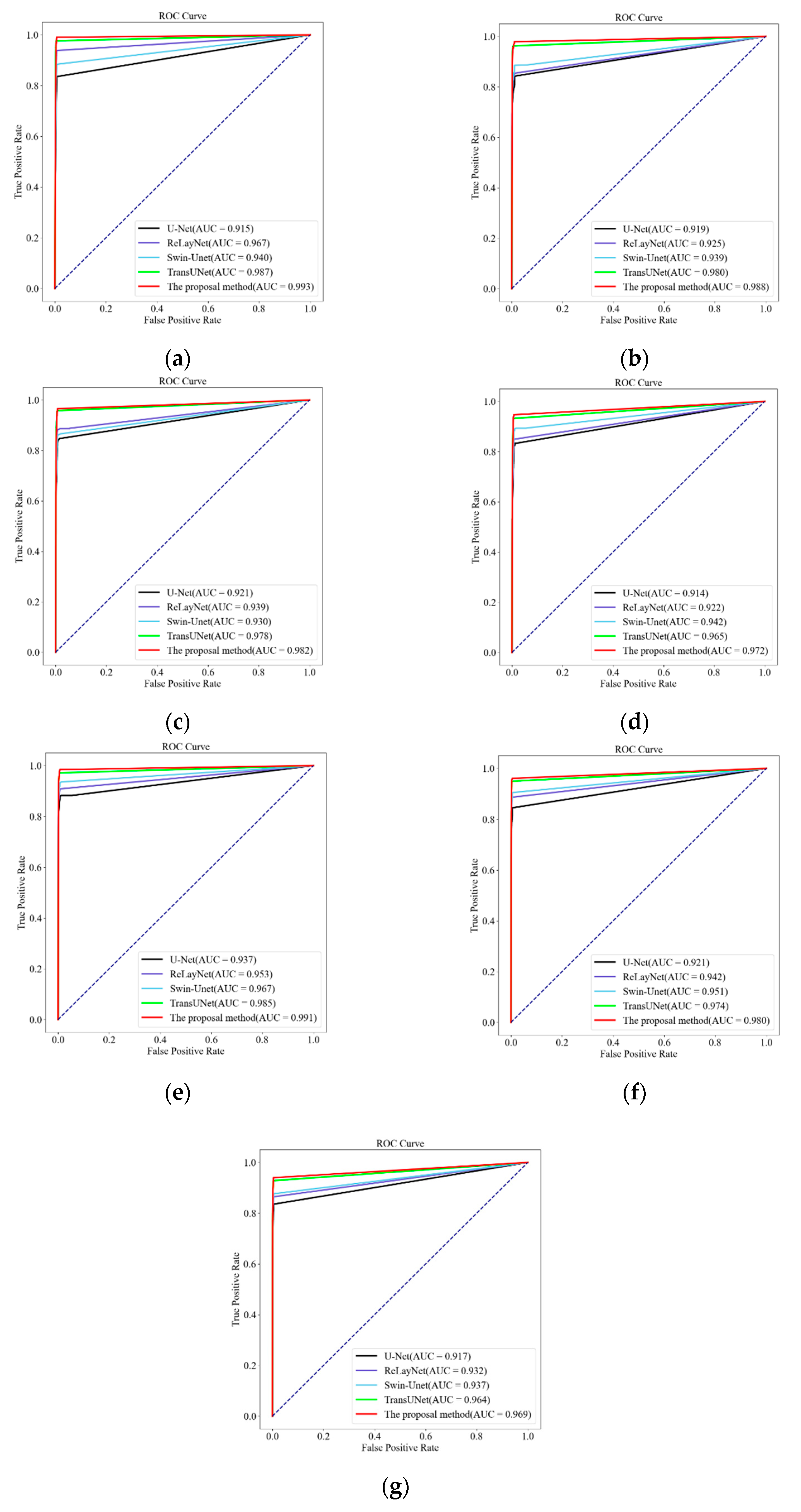
In order to further evaluate the predictive ability of the features, labels, and tests of different layers, for the seven-layer classification, each layer is regarded as an imbalanced binary classification problem, evaluated and visualized by the “Receiver Operating Characteristic” curve. The abscissa of the ROC curve is the false positive rate, and the calculation formula is (14). The ordinate of the ROC curve is the true positive rate, and the calculation formula is the same as the recall, that is, Formula (10). The ROC curves for U-Net, ReLayNet, Swin-Unet, TransUNet, and the proposed method were compared for the seven-layer segmentation of the retina, as illustrated in Figure 7, with the region below the ROC curve (AUC) as a metric for evaluating the model.

As shown in Figure 7, Figure 7a–g show the ROC curves of the results of this paper’s method (red line) and four other methods for segmenting the intraretinal layers of fundus OCT images in each layer, respectively. For different layers, the AUC values of different methods are shown in

Table 3. Comparison of AUC values of different methods in different layers.

Method	NFL	GCL-IPL	INL	OPL	ONL-ISM	ISE	OS-RPE
U-Net	0.915	0.919	0.921	0.914	0.937	0.921	0.917
ReLayNet	0.967	0.925	0.939	0.922	0.953	0.942	0.932
Swin-Unet	0.940	0.939	0.930	0.942	0.967	0.951	0.937
TransUNet	0.987	0.980	0.978	0.965	0.985	0.974	0.964
The proposed method	0.993	0.988	0.982	0.972	0.991	0.980	0.969

.

Table 3 describes the comparison results of the proposed method with U-Net, ReLayNet, Swin-Unet, and TransUNet in terms of AUC values. The AUC value of the proposed method in each layer is in the last row, which is higher than the four comparison methods on each layer.

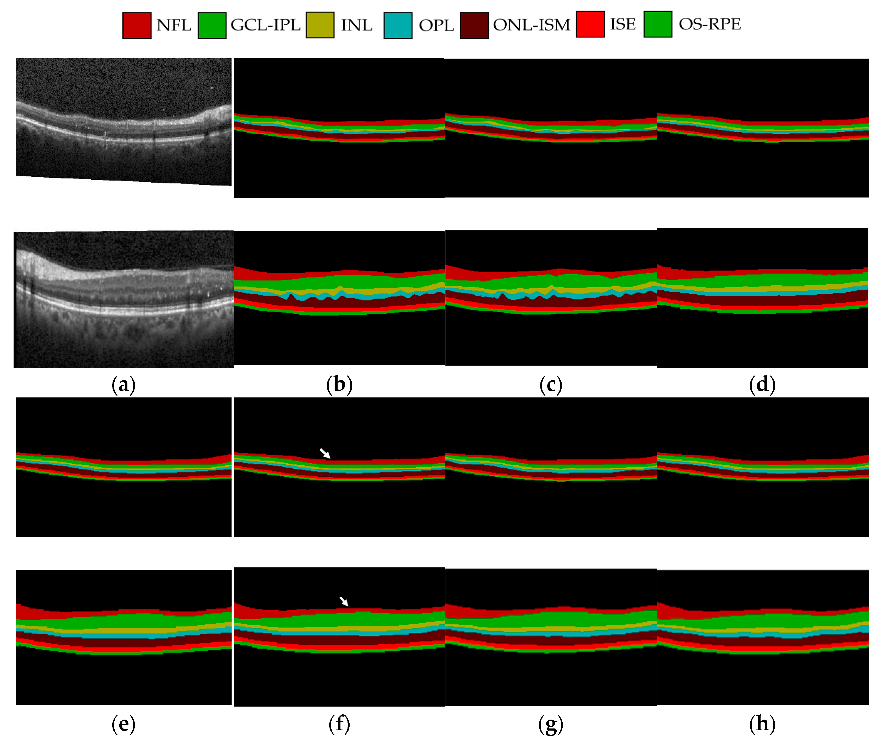
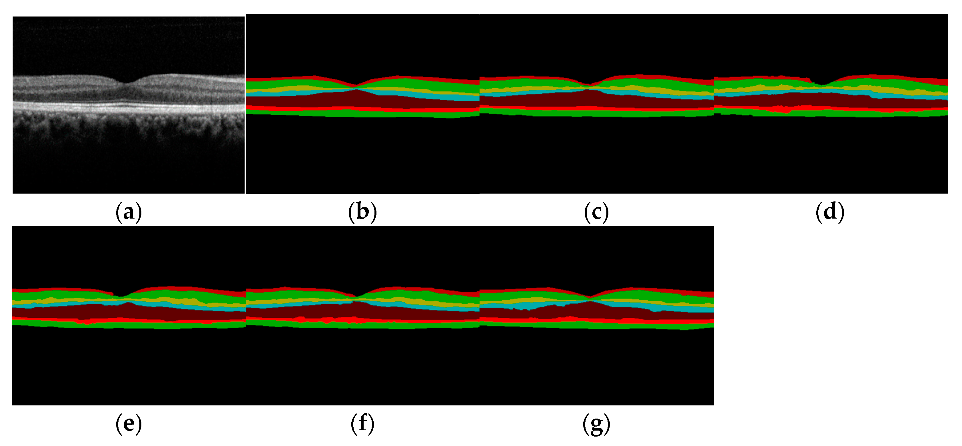
Figure 8 shows (a) the original image, (b) and (c) the labeled image of expert 1 and expert 2 respectively, (d) U-Net prediction results, (e) ReLayNet prediction results, (f) Swin-Unet prediction results, (g) TransUNet prediction results, and (h) the proposed method prediction results. As can be seen from the figure, the prediction results of U-Net network will be very fuzzy at the boundary, and the sense of boundary between layers is not so clear. The ReLayNet network does not have clear upper and lower boundaries when processing the OS-RPE layer. There are errors in the prediction results of the Swin-Unet network in the NFL layer, indicated by a white arrow in the figure. The prediction results of TransUNet network are relatively fuzzy at the boundary between the head and tail layers. The segmentation results of the proposed method are closer to the labeled image.

4. Discussion

To prove the generalization capability of the model, ablation experiments were performed to verify the significant performance of the RL-Transformer and Dense Block introduced in this paper. As shown in

Table 4. Characteristics of the baseline.

Method	RL-Transformer	Dense Block
Baseline 1	No	No
Baseline 2	Yes	No
Baseline 3	No	Yes
The proposed method	Yes	Yes

, the TransUNet is denoted as baseline 1, the TransUNet with RL-Transformer is denoted as baseline 2, and the TransUNet with Dense Block is denoted as baseline 3. The proposed method is TransUNet with RL-Transformer and Dense Block.

The quantitative results of the ablation experiment are shown in

Table 5. Quantitative comparison between Baseline 1-3 and the proposed method using Dice coefficient scores.

Method	NFL	GCL-IPL	INL	OPL	ONL-ISM	ISE	OS-RPE	Mean	Significance P
Baseline 1	88.41	92.21	84.06	82.55	94.03	89.04	86.43	88.10	-
Baseline 2	88.99	93.58	86.41	85.39	95.29	89.75	87.38	89.54	0.036
Baseline 3	89.26	92.27	84.51	84.19	94.29	90.75	89.68	89.27	0.027
The proposed method	90.72	93.93	86.8	85.38	95.72	91.47	88.88	90.41	0.029

. Comparing the results of baseline 1 and baseline 2, it can be seen that the Dice coefficient scores of each layer of baseline 2 are significantly better than the experimental results of baseline 1, indicating that RL-Transformer has a better effect on the intraretinal layer segmentation for OCT image. Comparing the results of baseline 1 and baseline 3, it can be found that the Dice coefficient scores of each layer of baseline 3 are better than those of baseline 1, which indicates that Dense Block can improve the layering segmentation effect of OCT images. Comparing the results of this paper’s method with those of Baseline 3, it can be seen that this paper’s method is better for each layer of the Dice coefficient score, indicating that the overall improvement of RL-Transformer and Dense Block has a better performance in improving the layering segmentation effect of OCT images. In summary, RL-Transformer and Dense Block have shown good performance in improving the segmentation of the intraretinal layer in fundus OCT images.

At the same time, taking baseline 1 as the standard, the paired t-test is conducted on baseline 2, baseline 3, and the proposed method to determine whether there is a significant difference between the two methods. The results show that all p-values are smaller than 0.05, showing a significant enhancement of the method in this paper.

As shown in Figure 9, the visualization result plot of the ablation experiment is illustrated. Figure 9a shows an original retinal OCT image with diabetic macular disease. It can be seen that the foveal area of the macular is obviously raised, and there are multiple cystic lesions with different sizes and irregular structures. Subfigure (c) shows the predicted layer segmentation result of baseline 1, and it can be seen that there are errors at the segmentation of INL and OPL layers, indicated by a white arrow in the figure. Subfigure (d) shows the predicted layer segmentation result of baseline 2, which is greatly improved compared with baseline 1, but there are still shortcomings in the left boundary and lesion area of the first layer. Subfigure (e) is the predicted layer segmentation result of baseline 3, and subfigure (f) is the predicted layer segmentation result of the proposed method. It can be seen that the boundary of the segmentation result is smooth and continuous, and it also has a good segmentation effect on the macular foveal lesion area.

The compared results of this paper’s method with the U-Net, ReLayNet, Swin-Unet, and TransUNet algorithms in terms of Params and Flops values and detection speed are shown in

Table 6. Speed comparison of different algorithms.

Method	Params(↓)	Flops(↓)	FPS(↑)
U-Net	37.65	57.26	35
ReLayNet	40.21	63.55	41
Swin-Unet	33.17	36.57	33
TransUNet	100.27	36.97	32
The proposed method	24.23	31.59	45

Note: ↑ indicates that a larger value is better, and ↓ indicates that a smaller value is better.

.

In Table 6, it can be seen that the proposed method is the lowest in both Params and Flops values, and the calculation amount is also the lowest when the number of parameters is reduced, indicating that replacing the original upsampling with Dense Block can reduce the calculation amount of the model and improve the calculation speed of the model. At the same time, the FPS value is also the highest, it shows that the method in this paper is better than other methods with regard to speed. The visualization results are shown in Figure 9.

Figure 10 shows (a) the results of comparing the number of parameters between this paper’s model and the comparison model, and (b) the results of comparing the computational volume between this paper’s model and the comparison model. The y-axis represents the DSC value (the higher the better), and the x-axis represents the Params (M) and Flops (G) (the lower the better), respectively. It is seen that the method proposed in this paper has the lowest Params and Flops values, while the DSC values are also higher than the other models, indicating that the method in this paper is faster and more accurate than the other methods in segmenting the intraretinal OCT images.

We also investigate the performance of the proposed method on the POne dataset. As mentioned above, the dataset contains 100 B-scans from 10 healthy adult subjects. The data set is used to verify and compare on U-Net, ReLayNet, TansUNet, and the method proposed in this paper, which further shows the generalization ability of the model proposed in this paper.

The results are shown in

Table 7. Quantitative comparison of Dice coefficients of the stratified results of each method on the POne dataset.

Method	NFL	GCL-IPL	INL	OPL	ONL-ISM	ISE	OS-RPE	Mean
Expert 2	0.852	0.913	0.798	0.812	0.947	0.791	0.831	0.849
U-Net	0.823	0.905	0.833	0.804	0.926	0.802	0.834	0.847
ReLayNet	0.867	0.912	0.840	0.821	0.935	0.842	0.877	0.871
TransUNet	0.913	0.940	0.853	0.857	0.961	0.913	0.920	0.908
The proposed method	0.921	0.946	0.872	0.883	0.973	0.927	0.930	0.922

. The comparison results of the proposed method with the dice overlap scores of the stratified results on dataset two of Expert 2, UNet, ReLayNet, and TransUNet are described. First, from the average of the overall dice overlap score, namely the last row of Table 7, the overall dice overlap score of the proposed algorithm is 0.922, which is better than 0.073, 0.075, 0.051, and 0.014 scores of expert 2 and the other three methods, respectively. Second, the dice overlap score in each layer is also slightly better than the other methods. Therefore, from the perspective of dice coefficient, the stratification results of the proposed algorithm are better than other methods.

As shown in Figure 11, (a) shows 1 original retinal OCT image on POne dataset, (b) and (c) represents the hierarchical results manually annotated by expert 1 and expert 2, respectively, and the annotations of each layer are also relatively complete and smooth; (d) is the predicted hierarchical result of U-Net method; (e) is the predicted hierarchical result of ReLayNet method; (f) is the predicted stratification result of TransUNet. It can be seen from (d), (e), and (f) that all three segmentation methods, U-Net, ReLayNet, and TransUNet, have broken in the first layer at the fovea of the retina, which is inconsistent with the annotation of expert 1. However, in (g) the proposed method obtains accurate and continuous and complete segmentation results in each layer, without fault phenomenon, and obtains better results.

5. Conclusions

In this paper, a novel lightweight TransUNet deep semantic segmentation network model was constructed for the intraretinal layer segmentation for fundus OCT image. The OCT dataset was augmented to improve the generalization of the model, and the Transformer was improved to an RL-Transformer to enhance the perceptual field and improve the coding ability of the model. Furthermore, changing the decoding layer to Dense Block could not only prevent the gradient explosion problem, but also better retain the context information, enhance the feature reuse, reduce the learning parameters, and reduce the computational burden. The SD-OCT and POne datasets are used to validate the model, and SD-OCT is a public dataset of Duke University. In recent years, Transformer is used in a variety of different medical image segmentation fields, and the application of Transformer in the field of retinal layer segmentation has also achieved good results. Subsequent work and research will focus on the research and implementation of fluid segmentation in choroidal and retinal diseases [29] and the lightweight of models [30].