Communication

Precise RF Phase Measurement by Optical Sideband Generation Using Mach–Zehnder Modulators

by
Qingchuan Huang
1,* and
Tetsuya Kawanishi
1,2
1
Department of Electronic and Physical Systems, Faculty of Science and Engineering, Waseda University, 3-4-1 Okubo, Shinjuku, Tokyo 169-8555, Japan
2
National Institute of Information and Communications Technology, 4-2-1 Nukui-Kita, Koganei, Tokyo 184-8795, Japan
*
Author to whom correspondence should be addressed.
Photonics 2023, 10(3), 324; https://doi.org/10.3390/photonics10030324
Submission received: 30 January 2023 / Revised: 8 March 2023 / Accepted: 15 March 2023 / Published: 17 March 2023

Abstract

:
A novel radio frequency (RF) phase measurement method that uses optical modulation was proposed. The mathematical model of Mach–Zehnder modulator (MZM) characterization was reviewed. By measuring the output sideband power of the optical modulator, the phase difference of the electric signals fed to the modulator was experimentally measured, and picosecond-level accuracies were achieved. This technique is expected to be useful for radio-over-fiber-based antenna array systems.

1. Introduction

In recent years, the application of video conferences and remote work has rapidly developed owing to the global pandemic. The increasing demand in the telecommunications industry requires increased transmission speed, larger bandwidth, lower latency, and ability to connect to more terminals. To utilize the currently unused high-frequency bands, research and studies aiming for beyond 5G (B5G) and 6G (6th generation wireless systems) telecommunication have begun. A demonstration of bidirectional 300 GHz terahertz transmission, which provides a transmission speed of 2 × 20 Gbps, has recently been experimentally performed [1].
One of the most significant applications contributing to the rapid development of communication technology is massive multiple input/multiple output (MIMO) antenna technology. Massive MIMO antennas can provide users with a high network capacity and improved coverage. With massive MIMO, uniform network access can be provided, similar to the realization of massive terminal connections. In the upcoming B5G and 6G networks, MIMO wireless technology is expected to play an important role. A photonics-aided 2 × 2 MIMO wireless THz wave signal transmission system was recently experimentally demonstrated, in which a 16 Gb/s 450 GHz polarization-division-multiplexed quadrature phase-shift keying (PDM-QPSK) signal was successfully transmitted over a 50 km wired SMF-28 link and a 142 cm wireless 2 × 2 MIMO link [2].
Radio-over-fiber (RoF) technology deployed in wireless networks can be used to increase transmission capacity and improve the quality of service. This provides a good balance between the flexibility and mobility of wireless access networks and the capacity of optical networks. The combination of RoF and MIMO has been experimentally demonstrated, realizing transmission in a 50 km SMF path length and a wireless distance of 15 m [3]. In recent research, the simulation of 60 GHz multiple input/multiple output generalized frequency division multiplexing (MIMO-GFDM) at 1 Gb/s and orthogonal frequency division multiplexing PON (OFDM-PON) signal at a 2.5 Gb/s data rate over a 20 km standard-PON span has also been reported [4]. This kind of result indicates that the system efficiency can be considerably enhanced by applying the combination of RoF and MIMO.
In general, a massive MIMO system is an expansion of a standard MIMO system. A standard MIMO system consists of two or four antennas, whereas a massive MIMO system is a combination of more than hundred antennas. To minimize radio frequency interference, the phase difference between each antenna element needs to be accurately measured and adjusted. In the case of massive MIMO, a large number of antennas increases the importance of accurately measuring the phase difference. A common method to measure the phase difference is to use a frequency domain measuring instrument, such as a vector network analyzer or a cross-domain analyzer.
Integrated lithium niobate (LN) modulators consisting of sub-Mach–Zehnder (MZ) interferometers arranged in parallel are commonly used for high-speed signal generation [5]. Through the characterization of Mach–Zehnder modulators, the working state of the MZM can be systematically verified. By measuring the power of the optical output sidebands, the change in the electrical signal could be derived and verified from the change of the optical signal. Based on this property, the phase difference of the electric signals fed to the modulator can be evaluated through an optical spectrum analysis.
In this study, the phase difference of the modulating signals between the two paths of a Mach–Zehnder modulator was experimentally measured using optical spectrum analysis. Compared with the conventional method, the measurement error based on the optical spectrum analysis of the MZM produces more accurate results, with an error smaller than a few picoseconds in the time domain. This method is an effective technique for supporting massive MIMO antenna array systems. The reminder of this paper is organized as follows: Chapter 2 reviews the MZM characterization calculation model and presents the experimental setup. The experimental results and discussion are presented in Section 3. Finally, Section 4 presents the conclusion of this research.

2. Methods

2.1. Characterization of Mach–Zehnder Modulator

The parameters of a given MZM can be measured by feeding its electrodes with an electrical signal in a push–pull scheme, and the corresponding optical sideband components can be generated and measured [6]. The optical spectrum analysis of the MZ modulator can be used to characterize the MZ modulator. In this type of optical spectrum analysis, the carrier component can be ignored, whereas the maximum and minimum power intensities of the sideband are measured. The output power of nth-order optical sideband components from the MZ modulator can be expressed as [7]
P n = K 2 4 | J n ( A 1 ) I 1 + J n ( A 2 ) I 2 e i ( n ϕ + B ) | 2
where K donates the total insertion loss of MZM, and J n is the first kind of nth-order Bessel function. B is defined as the optical phase difference induced by an applied DC bias voltage. For the common MZM, it is necessary to properly set the average voltage of the modulating signal, which fluctuates alternately. This average voltage is called the DC bias or simply the bias of the modulator [8]. ϕ is the skew that describes the phase difference deviation of the modulating signals in relation to the ideal push–pull condition. A i is the optical phase shift induced by the sinusoidal signal at the i -th interferometer ( i = 1 , 2 ) of MZM.
A 1 =   A 1 + α 0
A 2 =   A 1 α 0
α 0 is defined as the intrinsic chirp parameter; η describes the power imbalance between two interferometers. A is the modulation depth at each arm of the MZM. I i is defined as the optical power imbalance at the i -th interferometer ( i = 1 , 2 ), which can be expressed as:
I 1 = 1 + η 2
I 2 = 1 η 2
By applying a DC bias voltage, the optical phase differences of B k = 0 and B k = π can be induced. Therefore, the maximum and minimum intensities of each sideband component are measured. The ( + ) sign indicates the maximum sideband value, whereas the ( ) sign indicates the minimum sideband value. The parameters A , α 0 , and η can then be derived from the following calculation: First, the approximate value of A can be calculated using Equation (6):
P m + P n + J m A J n A 2
In optical spectrum analysis, the measured sideband components with lower order are preferred because their power is generally larger than that of the higher-order components. P 1 + and P 2 + are usually used for the calculation, and by substituting P 1 + and P 2 + into Equation (6), the approximate value of A can be calculated. After that, approximate values of α 0 and η can be obtained from the following expression:
P n P n + = η 2 + A α 0 J n 1 A J n A n A 2  
The ratios of first- and second-order sidebands P 1 / P 1 + and P 2 / P 2 + can be applied to Equation (7). Generally, two unknown parameters can be derived from these two equations. Several solutions, including unphysical solutions, are derived for these transcendental equations. High-order sideband components, such as P 3 and P 3 + , should be used to determine which solutions are physically possible.
The precision of calculation can be improved through the following equation: [9]
P n , k P n , k + = J n ( A 1 ) I 1 J n A 2 I 2 J n ( A 1 ) I 1 + J n ( A 2 ) I 2 2
The sideband intensities P 1 ,   P 1 + ,   P 2 ,   P 2 + ,   P 3 , and P 3 + can be substituted into Equation (8) for calculation. However, considering the actual measurement, the intensity of third-order sideband may be too low to be detected. Ratio of P 1 / P 1 + ,   P 2 / P 2 + , and P 1 + / P 2   + can also be considered. Therefore, three equations can be obtained to solve the three unknown parameters, and A , α 0 , and η k calculated before can be used as the initial values for the final calculation. The insertion loss K can also be calculated using expressions of A i and I i :
P n , k + = K 2 4 [ J n A 1 I 1 + J n A 2 ) I 2
The characterization method provides an effective way to determine the MZM parameters. By monitoring the modulation depth A , chirp parameter α 0 , and optical power imbalance η , the current working state of the MZM can be studied from the instant sideband components and current bias phase B , and the phase difference ϕ can be calculated.
Referring to Equation (1), the nth-order optical output sideband component of the MZM can also be written in the form:
P n = K 2 4 J n 2 A 1 I 1 2 + J n 2 A 2 I 2 2 + 2 cos n ϕ + B J n A 1 J n A 2 ( 1 η 2 4 )
The intensities of the upper and lower sidebands of the first- and second-order components P 1 ,   P 1 , P 2 , and P 2 were measured using an optical spectrum analyzer. The instant skew ϕ and bias phase B can be directly obtained by solving Equations (11) and (12).
P 1 P 1 = J 1 2 A 1 I 1 2 + J 1 2 A 2 I 2 2 + 2 c o s B + ϕ J 1 A 1 J n A 2 ( 1 η 2 4 ) J 1 2 A 1 I 1 2 + J 1 2 A 2 I 2 2 + 2 c o s B ϕ J 1 A 1 J 1 A 2 ( 1 η 2 4 )
P 2 P 2 = J 2 2 A 1 I 1 2 + J 2 2 A 2 I 2 2 + 2 c o s B + 2 ϕ J 2 A 1 J n A 2 ( 1 η 2 4 ) J 2 2 A 1 I 1 2 + J 2 2 A 2 I 2 2 + 2 c o s B 2 ϕ J 2 A 1 J n A 2 ( 1 η 2 4 )
Owing to the property of the trigonometric equation, the 360-degree shift in the measured skew ϕ and bias phase B should be carefully checked and verified. Setting an initial value for the calculation can help determine appropriate solutions.

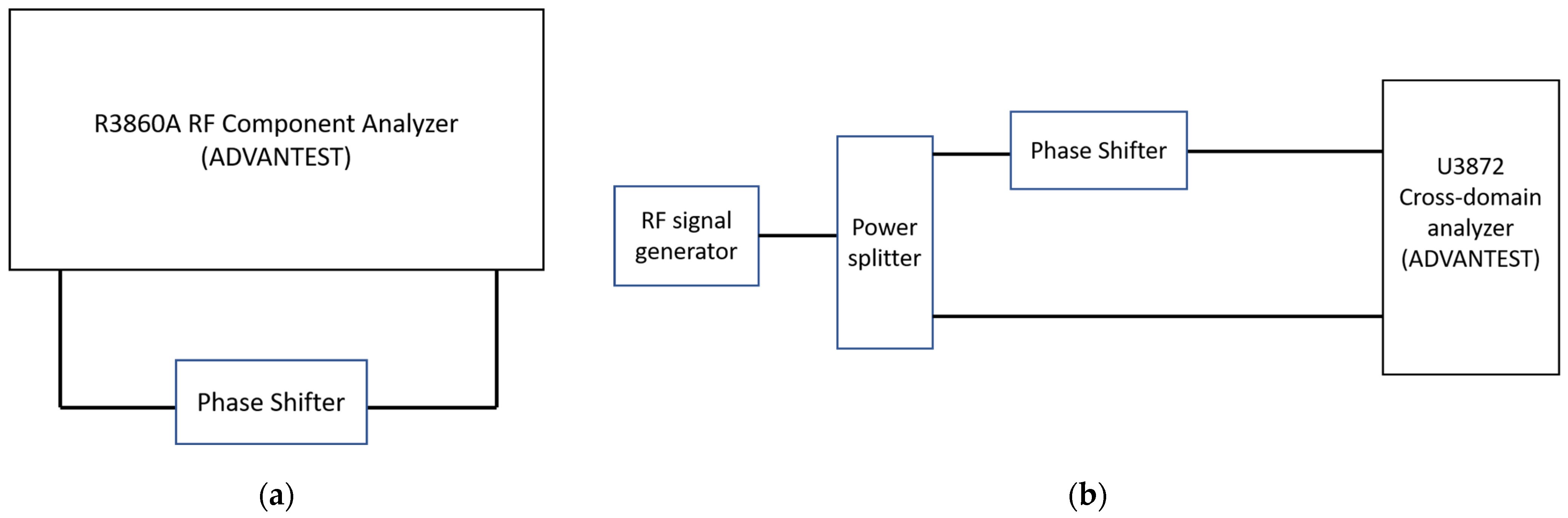
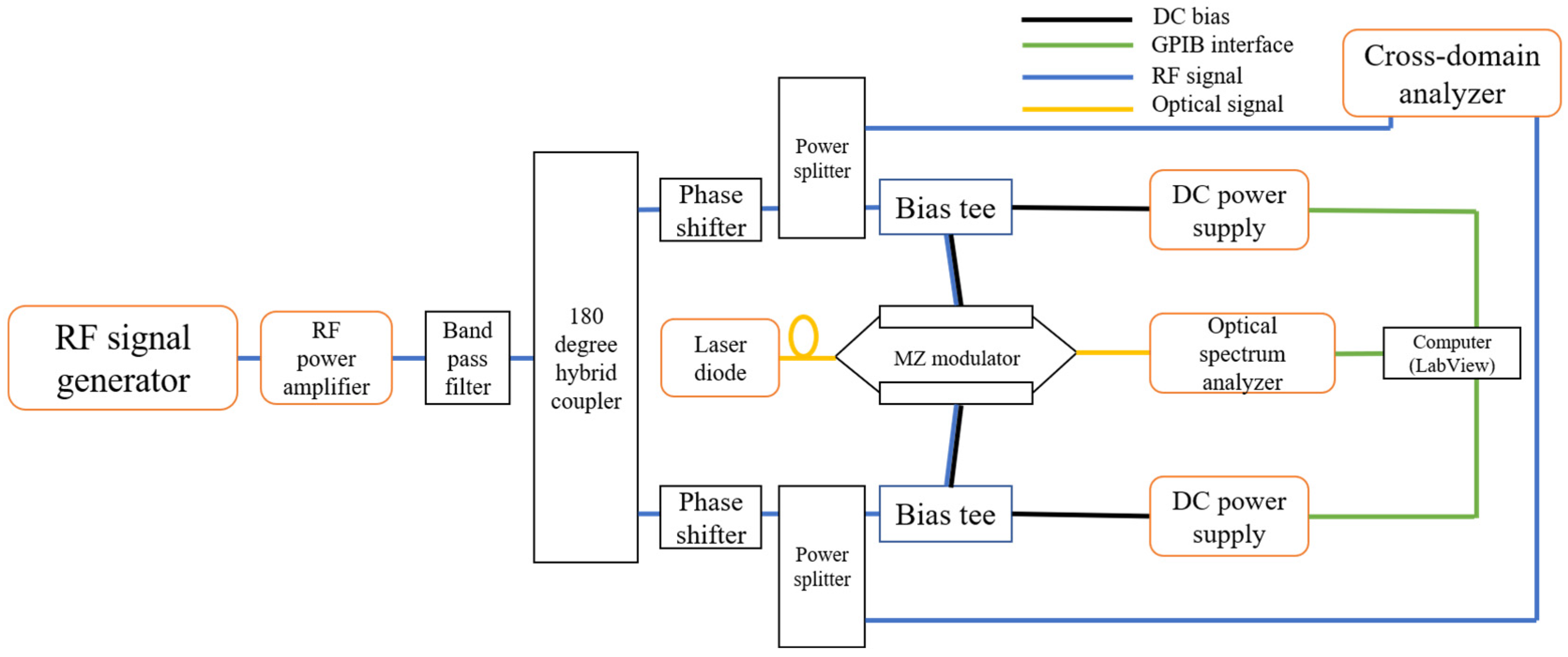
2.2. Experimental Setup

A single MZM with two electrodes on two subphase modulators was used in this experiment. As shown in Figure 1, the experimental setup consisted of four parts: signal generation, reference, single MZM, and signal processing. The brands and models of the instruments used in this experiment can be found in Appendix A. The signal generation part includes the signal generator, RF power amplifier, and the band-pass filter. An RF signal generated by signal generator was used as the modulating signal, which was pumped by the RF power amplifier and then purified by the band-pass filter. The band-pass filter can prevent the high-frequency synchronized components and nonlinear components generated by the RF power amplifier from affecting the measurement results.
The reference part in this configuration can be used to measure the RF phase difference as the reference value. The power dividers in the circuit divide the input electronic signals into two parts. Half of the input signal is fed to the MZM modulator, and the other half is connected to the cross-domain analyzer for the RF phase measurement. The cross-domain analyzer (CDA) is a kind of two-channel vector and spectrum analyzer. This device can enable comparative real-time RF phase measurements from the two channels over a wide frequency range [10].
A single LN-based MZM with two electrodes was used in this experiment. A grid-tunable laser source (TLS) was used to provide the input optical signal. The DC power source can generate the DC signal, which is used to change the bias state of the MZM. The bias tee was used to combine the input RF signal and DC signal.
The signal processing part included an optical spectrum analyzer and PC. The intensity of the output optical sideband was recorded using an optical spectrum analyzer. The calculation of the instant RF phase change was realized using a PC. In this experiment, the DC bias source and the optical spectrum analyzer were connected through a GPIB interface.
First, the relationship between the measured bias phase and measured RF phase difference needs to be confirmed because the bias condition fluctuates in the time domain owing to the DC drift and heat effect. A larger initial bias voltage accelerated the DC drift; thus, the half-wave voltage range with a smaller DC bias voltage was used [11]. The full-bias-states and null-bias states should be found before. The DC bias voltage was adjusted to 0.1 V per step, and the corresponding RF phase difference was recorded. Therefore, the stability of the measured RF phase is confirmed.
Calibration of the cross-domain analyzer should be conducted later. After generating a ramp signal by the DC bias source, first-, second-, and third-order sideband components will be swept under a range of two times the half-wave voltage. The computer is then applied to the measurement of sideband data and the calculation of the working parameters of MZM with LabView and MATLAB. Finally, after the characterization of the MZM, the instant sideband power can be measured and used to figure out RF phase difference.
To further verify the reliability of the measured RF phase using optical spectrum analysis, the RF phase difference measured by the CDA was used as the reference data. A comparison of the measurement results and measurement errors was quantitatively analyzed and will be provided later.

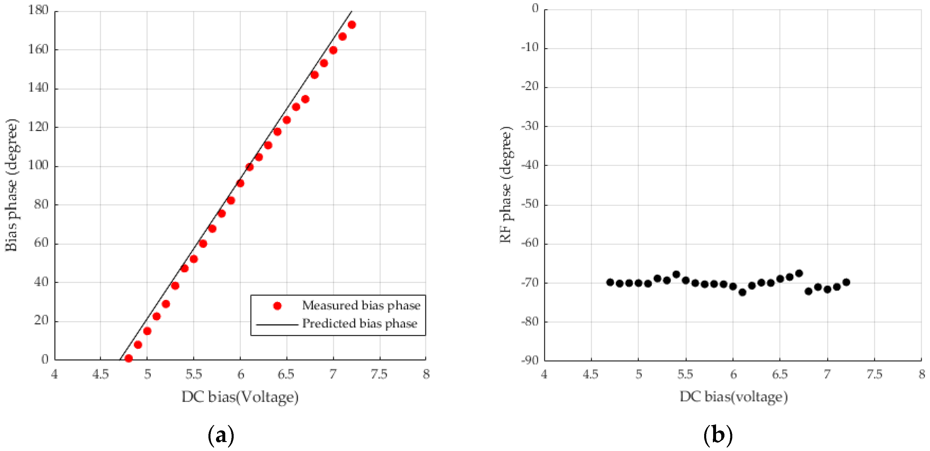
3. Results and Discussion

Figure 2a shows the relationship between the measured bias phase and the DC bias voltage. The change in the measured RF phase difference when a DC bias was applied is shown in Figure 2b. The bias phase changed linearly, whereas the measured RF phase was maintained at a stable level. This result indicates that the measured RF phase was not influenced by the bias fluctuation.
The RF signals of 12, 12.5, and 13 GHz were used as modulating signals in this experiment. The DC bias voltage exerted on the electrodes is set around a 90 ° bias phase state.
Avoiding the use the full-bias and null-bias states is very significant because an asymmetric sideband is needed. After calibrating the CDA, the initial phase difference was set as close to zero. By referring to the phase difference shown on the CDA, the phase shifter was rotated to change the skew by approximately 5 ° each time. It is difficult to maintain the same measurement step because phase shifters have unavoidable mechanical limitations. The current RF phase difference and bias phase can be measured by performing the characterization method and recording the instant sideband power. The RF phase difference was measured for at least 5 times, and the average values were recorded in order to suppress the influence from the fluctuation of the optical sideband.
Figure 3a shows the phase measurement results at 12 GHz. Figure 3b shows the absolute measurement error between the two types of measurement. The x-axis is the measured phase difference from the CDA, whereas the y-axis is the result obtained from the optical spectrum analysis. The red curve represents the reference phase curve measured by the CDA. The error bars show the phase measurement variation range of the CDA. The measured data points located near the reference curve were considered more accurate. The absolute measurement error was smaller than 4 ° .
Measurements were conducted at different frequencies to confirm the measurement stability by changing the frequency of the modulating signal. The phase difference measurement results at 12.5 GHz are shown in Figure 4a. Figure 4b shows that the absolute measurement error was suppressed under 7 ° . The absolute measured error between the results from the CDA and the results from the MZM is larger than the error under 12 GHz.
Following the same procedure, an experiment under 13 GHz was also conducted. Figure 5a shows the phase measurement results, whereas the absolute error is shown in Figure 5b. A comparison of the three different measurements is presented in Table 1.
Table 1 shows that the absolute measurement error was less than 10 degrees in the three groups of measurements. The measurement error under 12.5 GHz is larger than that of the other two groups of measurements. There are several possible explanations for this finding. First, the instant bias phase and RF phase difference were calculated from the sideband intensity. The output power measured by the optical spectrum analyzer occupied the dominant position in whole measurement. Thus, the fluctuation induced by the optical spectrum analyzer cannot be neglected. This problem can be solved by applying the average value of the sideband intensity for the calculation. The stability of the laser diode should also be considered here. However, the grid TLS used in this experiment provided the relatively stable output. The wavelength stability is ± 2.4 pm under 1550 nm, and the variation of optical output level is ± 0.03 dB [12]. The effect of minor fluctuations from the laser diode could be neglected in the measurement. Furthermore, the variation of the phase measured by the CDA would be ± 6 ° . (The discussion can be found in Appendix B) Thus, the reference value may not be sufficiently precise.
In this experiment, the testing instrument used was only adapted for low frequencies, and the sampling speed of the optical spectrum analyzer was relatively low. However, the overall measurement error was successfully suppressed below 10 degrees, allowing several picosecond-level accuracies to be achieved.

4. Conclusions

In this study, a phase difference measurement of the MZM using optical spectrum analysis is proposed. Through characterization of the MZM, the working parameters of the MZM can be identified, allowing the instant bias phase and skew change to be calculated from the sideband component of the optical output. The phase measurement method was experimentally demonstrated. The measurement of the bias phase and RF phase indicates that this method has sufficient tolerance for bias fluctuation. A cross-domain analyzer was used as a reference to confirm the accuracy of the phase measurement. The absolute measurement error was smaller than 10 ° during the test, providing a precise measurement in which the error was smaller than 2.3 ps in the time domain. This technique is expected to be useful for radio-over-fiber-based antenna array systems.

Funding

This paper includes research results from works funded by the Commissioned Research (No. 04901 and No. 06001) of National Institute of Information and Communications Technology (NICT), Japan, and also results from research supported by JSPS KAKENHI Grant Number JP22H05196.

Informed Consent Statement

Not applicable.

Data Availability Statement

Not applicable.

Conflicts of Interest

The authors declare no conflict of interest.

Appendix A

The following instruments were used in the experiment:
  • RF signal generator: ROHDE & SCHWARZ SMF 100A;
  • Optical spectrum analyzer: YOKOGAWA AQ6370N;
  • DC power supply: ROHDE & SCHWARZ HMC8043;
  • Phase shifter: SAGE 6705K-2;
  • Laser diode: YOKOGAWA AQ2211 frame controller with AQ2200-132 grid TLS module;
  • Cross-domain analyzer: ADVANTEST U3872.

Appendix B

According to the datasheet, the phase measured by the CDA has a variation of ± 15 ° under the worst conditions. Even though the manufacturer tends to set a larger specification for measurement instruments, a series of measurements for confirming the accuracy of the cross-domain analyzer is still needed to be verified. A vector network analyzer (VNA) was used to compare RF phase measurement accuracy with the CDA.
Figure A1a shows the experimental setup of the VNA, and the experimental setup of the CDA is in Figure A1b. A phase shifter was used to induce the phase change in the circuit. The initial phase of the phase shifter is defined as phase A. The phase shifter was adjusted to induce two different phase states. The changed phase is defined as phase B and phase C.
Figure A1. (a) RF phase measurement by VNA (b) RF phase measurement by CDA.
Photonics 10 00324 g0a1
Table A1 shows the phase measurement results by the VNA, whereas Table A2 shows the phase measurement results by the CDA. Table A3 describes the difference in the measured phase between the VNA and the CDA.
Table A1. Phase measurement results by VNA.
FrequencyPhase A to Phase BPhase B to Phase C
12 GHz 15.1 ° 17.9 °
12.5 GHz 18.5 ° 15.5 °
13 GHz 18 ° 15 °
Table A2. Phase measurement results by CDA.
FrequencyPhase A to Phase BPhase B to Phase C
12 GHz 14.89 ° 17.52 °
12.5 GHz 16.53 ° 15.82 °
13 GHz 17.39 ° 15.85 °
Table A3. Difference in measured phase between VNA and CDA.
FrequencyPhase A to Phase BPhase B to Phase C
12 GHz 0.21 ° 0.38 °
12.5 GHz 1.97 ° 0.32 °
13 GHz 0.61 ° 0.85 °
According to the results shown in Table A3, the difference in the measured phase is smaller than ± 2 ° under 12, 12.5, and 13 GHz. The dynamic phase measurement accuracy of the VNA is within ± 4 ° in the frequency range of 8 to 20 GHz [13]. This result indicates that the CDA can provide the phase measurement with an accuracy of ± 6 ° in the frequency range of 12 to 13 GHz.

References

  1. Succeeded in the World’s First Bidirectional 300 GHz Terahertz Transmission. Available online: https://www.waseda.jp/top/news/81671 (accessed on 25 January 2023).
  2. Yu, J. Terahertz Signal MIMO Transmission. In Broadband Terahertz Communication Technologies; Springer: Berlin/Heidelberg, Germany, 2021; pp. 99–120. [Google Scholar]
  3. Amiri, I.S.; Alavi, S.E.; Fisal, N.; Supa’at, A.S.M.; Ahmad, H. All-Optical Generation of Two IEEE802.11n Signals for 2 × 2 MIMO-RoF via MRR System. IEEE Photonics J. 2014, 6, 1–11. [Google Scholar] [CrossRef]
  4. Raji, Y.M.; Dahawi, T.H.; Yusoff, Z.; Senior, J.M. 60GHZ MIMO-GFDM RoF Over OFDM-PON. In Proceedings of the 2022 IEEE 9th International Conference on Photonics (ICP), Kuala Lumpur, Malaysia, 8–10 August 2022. [Google Scholar]
  5. Kawanishi, T.; Sakamoto, T.; Chiba, A. High-speed vectorial lightwave modulation techniques. In Proceedings of the 2008 Digest of the IEEE/LEOS Summer Topical Meetings, Acapulco, Mexico, 21–23 July 2008. [Google Scholar]
  6. Kawanishi, T.; Kogo, K.; Oikawa, S.; Izutsu, M. Direct Measurement of chirp parameters of high-speed Mach-Zehnder type optical modulators. Opt. Commun. 2001, 195, 399–404. [Google Scholar] [CrossRef]
  7. Kawanishi, T. Estimation of Parallel Mach-Zehnder Modulators. In Electro-Optic Modulation for Photonic Networks: Precise and High-Speed Control of Lightwaves; Springer: Berlin/Heidelberg, Germany, 2022; pp. 205–211. [Google Scholar]
  8. Kawanishi, T. Basics of Electro-Optic Modulators. In Electro-Optic Modulation for Photonic Networks: Precise and High-Speed Control of Lightwaves; Springer: Berlin/Heidelberg, Germany, 2022; pp. 62–63. [Google Scholar]
  9. Hugo, S.C.; Freire; Yamaguchi, Y.; Kawanishi, T. High-Speed Characterization of Parallel Mach-Zehnder Optical Modulators. In Proceedings of the 2019 24th OptoElectronics and Communications Conference (OECC) and 2019 International Conference on Photonics in Switching and Computing (PSC), Fukuoka, Japan, 7–11 July 2019. [Google Scholar]
  10. U3841/3851/3872—Advantest. Available online: https://www3.advantest.com/documents/11348/146302/catalog_U3841_U3851_U3872_e.pdf/6a412e3e-fcd7-44ed-8ae0-5474865c4fe4 (accessed on 25 January 2023).
  11. Nagata, H.; Honda, H.; Akizuki, K. Initial bias dependency in dc drift of z-cut LiNbO3 optical intensity modulators. Opt. Eng. 2000, 39, 1103–1105. [Google Scholar]
  12. AQ2200 Series Multi Application Test System—Yokogawa. Available online: https://cdn.tmi.yokogawa.com/1/2474/files/BUAQ2200-20EN.pdf (accessed on 4 March 2023).
  13. R3860A RF Component Analyzer—Advantest. Available online: https://scdn.rohde-schwarz.com/ur/pws/dl_downloads/dl_common_library/dl_brochures_and_datasheets/pdf_1/R3860A_R3768_R3770.pdf (accessed on 3 March 2023).
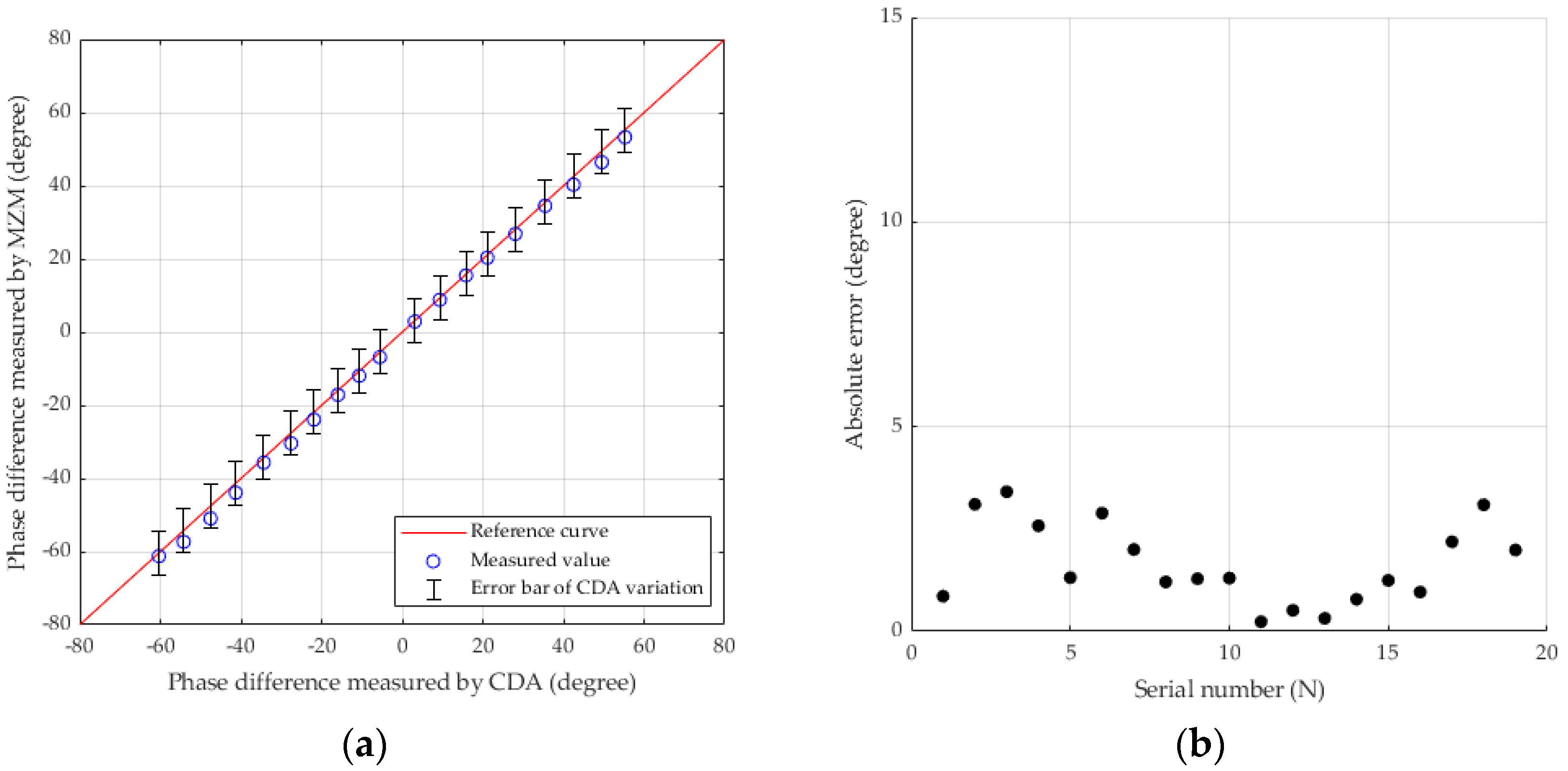
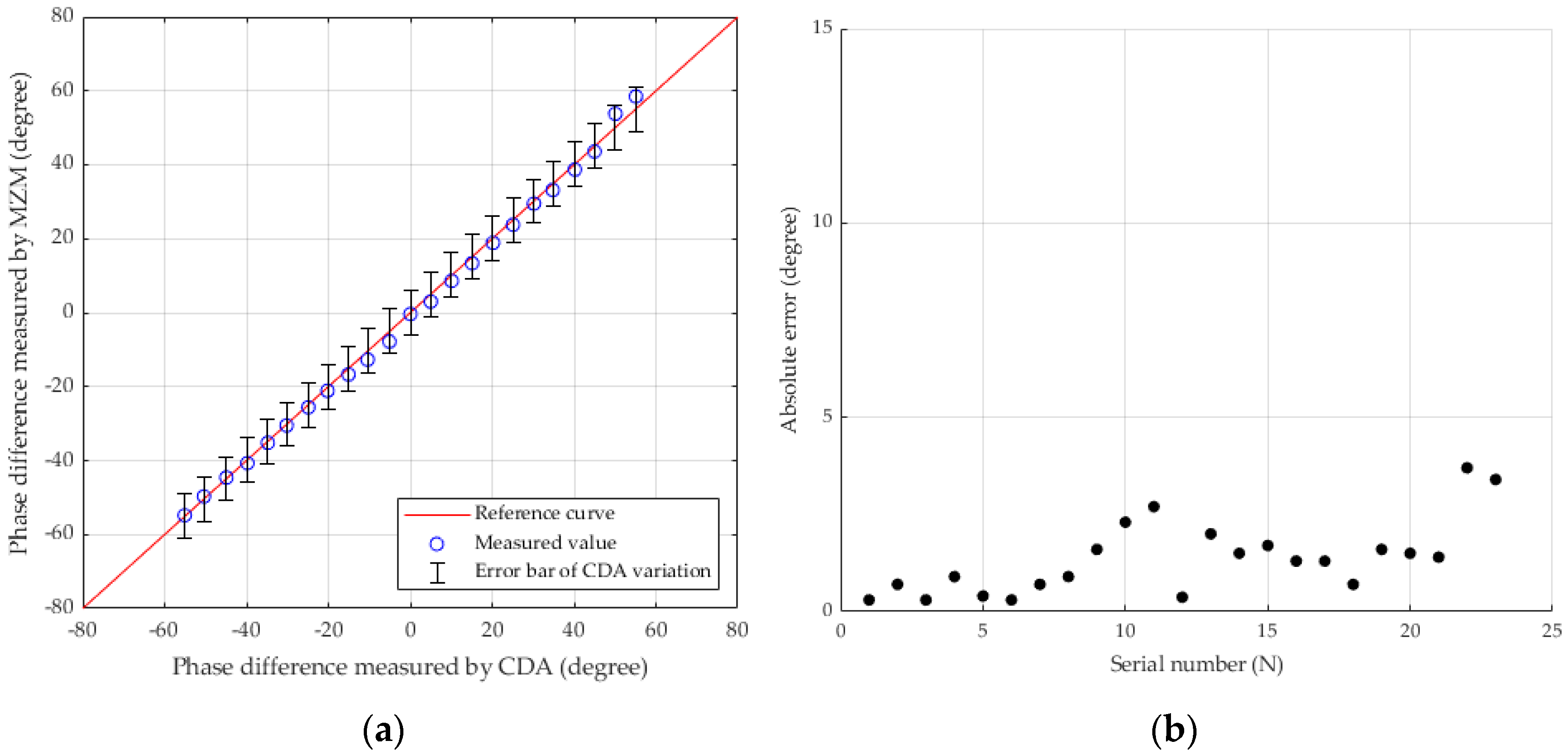
Figure 1. Experimental setup for phase difference measurement.
Photonics 10 00324 g001
Figure 2. (a) Relationship between measured bias phase applied and DC bias voltage; (b) Relationship between measured RF phase and applied DC bias voltage.
Photonics 10 00324 g002
Figure 3. Phase difference measurement under 12 GHz (a) RF phase difference from MZM and CDA; (b) Absolute measurement error between two measurements.
Photonics 10 00324 g003
Figure 4. Phase difference measurement under 12.5 GHz (a) RF phase difference from MZM and CDA; (b) Absolute measurement error between two measurements.
Photonics 10 00324 g004
Figure 5. Phase difference measurement under 13 GHz (a) RF phase difference from MZM and CDA; (b) Absolute measurement error between two measurements.
Photonics 10 00324 g005
Table 1. Relationship between modulating frequency and absolute error.
Modulating FrequencyAbsolute ErrorAbsolute Error (Time Domain)
12 GHz<4 ° <0.93 ps
12.5 GHz<7 ° <1.56 ps
13 GHz<5 ° <1.07 ps
Disclaimer/Publisher’s Note: The statements, opinions and data contained in all publications are solely those of the individual author(s) and contributor(s) and not of MDPI and/or the editor(s). MDPI and/or the editor(s) disclaim responsibility for any injury to people or property resulting from any ideas, methods, instructions or products referred to in the content.

