LIMPID: A Lightweight Image-to-Curve MaPpIng moDel for Extremely Low-Light Image Enhancement

Abstract

Low-light conditions severely degrade the captured image quality with few details, while deep learning approaches are trending towards low-light image enhancement (LLIE) due to their superior performance. However, few methods face the challenges of lower dynamic range and greater noise from extremely low-light directly. Existing methods for extremely low-light enhancement are end-to-end, requiring RAW data as input. Meanwhile, they often lack the potential for real-time mobile deployment owing to the high model complexity. In this paper, we introduce the image-to-curve transformation to ELLIE for the first time and present a Lightweight Image-to-curve MaPpIng moDel for ELLIE (LIMPID). Compared with existing image-to-curve mapping methods, the proposed module is constructed for a wider dynamic range according to the light scattering model. Furthermore, we propose a new pyramid fusion strategy based on Laplacian and Gaussian. This strategy attempts to achieve dynamic fusion of multi-scale images via learnable fusion weight parameters. Specifically, LIMPID consists of a low-resolution dense CNN network stream and a full-resolution guidance stream. First, the curve generation and refinement are achieved in the low-resolution stream constructed on a light scattering model. Then, the curves are up-sampled to full resolution via bilateral grid cells. Finally, the enhanced result is obtained through dynamically adapted multi-scale pyramid fusion. Experimental results show that our method is competitive with existing state-of-the-art methods in terms of performance.

1. Introduction

High-level vision tasks, such as object detection and identification, have made substantial progress in this decade and rely primarily on the quality of the input images. Despite the continued advances in camera sensors and image signal processing pipelines of digital photography, low light conditions are still a challenge due to environmental degradation factors (inadequate lighting conditions, etc.). These low-quality images lose information in the dark areas and suffer from unanticipated noise and color bias, reducing information transmission accuracy and resulting in incorrect object detection or identification. As a result, a growing amount of attention has been paid to LLIE. In particular, picture quality further degrades in extremely low-light scenes, where lower dynamic range and greater noise can pose greater challenges for image enhancement and recovery.

Deep learning methods have been the new trend for LLIE solutions in this decade, as computational resources have great improvement. Usually, end-to-end methods convert low-light images to enhanced images as output. End-to-end methods [1,2,3] are used to directly learn the transformation from the input to the corresponding output image, amongst which numerous methods [4,5] are often combined with Retinex theory to achieve better performance, with the enhancement of image components being performed on separate sub-networks introduced in [3,6]. The derivative works include adding a noise decomposition module by RRDNet [7] or a multi-scale luminance attention module [8]. Similarly, some approaches design different sub-networks to solve specific degenerate entanglement problems. Atoum et al. [9] and Li et al. [10] used different repair strategies to enhance luminance and chrominance, respectively, and Hu et al. [11] specialized in denoising and color correction. Another category of methods focuses on the uncertain nature of LLIE, thus taking complete account of different lighting conditions as well as user preferences [12,13,14,15].

Nevertheless, only rare methods have tackled the enhancement of extremely low-light images. Chen et al. [16] proposed a learning-based method that uses a CNN to directly convert an extremely low-light RAW image to a good-quality RGB image. Wei et al. [17] explained how to construct more realistic noise data for noise reduction in extremely low light. However, all these methods use RAW images as input in order to obtain more complete image information, a requirement that limits the application scenarios of the methods to some extent. Moreover, these aforementioned methods are also end-to-end-based, which generally incurs high computational costs linearly proportional to the input size, as they consist of a large number of stacked convolutions. Therefore, this expressiveness comes at the cost of computing, making it hard to apply to real-time devices.

A new category of deep learning methods, called image-to-curve mapping, obtains inspiration from art design or painting. In these applications, human image retouchers frequently employ professional software such as Photoshop to manually promote the development of digital photographs’ aesthetic quality. Users often alter an S-curve that specifies a function from the input level of a particular color channel to the output level for typically remapping the hue of an image. For example, moving a point up or down will lighten or darken a tonal area. However, manual enhancement can still be challenging for non-professionals who may lack the appropriate skills, time, or aesthetic judgment to efficiently improve the visual perception of their photographs. Therefore, a deep learning-based solution to mimic professional image-to-curve retouching becomes a huge challenge.

To tackle the challenges mentioned above, the image-to-curve approach is proposed as an image enhancement strategy that greatly simplifies the network and speeds up the overall process compared to pixel-by-pixel reconstruction. It simply requires a number of curve parameters to be estimated. In recent years, the efficacy of image-to-curve has been proven in existing LLIE methods [18,19,20,21,22]. One of the most widely noticed is the recently proposed Zero-DCE [21], which uses a low-light image as an input and generates high-order curves as outputs. These curves can be adjusted at a pixel level for enhancement over the varying range of the input, while at the same time preserving the details and intrinsic relationships among surrounding pixels. Since the curve is considered to be microscopic, its adjustable parameters are can be learned by a neural network. Therefore, image-to-curve mapping provides a lightweight solution for learning pixel adjustment over a wide dynamic range. Aiming at a highly efficient solution for ELLIE, we introduce a light scattering model to design a curve refinement module to reshape the training-learned curve, achieving a wider dynamic range. We also use a 3D upsampling approach, inspired by HDRNet [23], to store the curve parameters in bilateral grid cells, further refining the smoothness of the mapped curve. In the full-resolution stream, a proposed automatic fusion strategy optimizes high-frequency and low-frequency information adaptively via a refined version of Gaussian and Laplacian pyramidal fusion. LIMPID is the first attempt to apply image-to-curve mapping to ELLIE and our main contributions are three-fold:

• We introduce image-to-curve mapping to extremely low-light enhancement for the first time.
• We design a lightweight network for real-time extremely low-light image enhancement.
• We propose an adaptive multi-scale fusion strategy in terms of color and texture optimization.

2. Related Work

The advent of big data and computing resources such as GPUs has led to the rapid development of deep learning, which has begun to achieve impressive results in LLIE and has become mainstream in recent years, benefiting from superior enhanced performance and faster speeds than traditional methods. These solutions can be divided into two main categories: end-to-end and image-to-curve approaches.

2.1. End-to-End Methods

End-to-end solutions convert the low-light image into an enhanced image as the output and are often combined with Retinex models [24], which usually separately enhance the luminance component and the reflectance components via specialized sub-networks. KinD [3] was inspired by Retinex to decompose the image into two components: the luminance component is responsible for light adjustment, and the reflection component is responsible for removing degradation. KinD++ [8] is an improved version on aspects of the design of a new multi-scale illumination attention module in order to further improve the enhanced quality of KinD [3]. Zhang et al. [25] proposed a new Retinex model based on maximum information entropy, which achieves self-supervised learning by introducing the constraint that the maximum channel of reflectance matches the maximum channel of low-light images. The Retinex model usually ignores the noise, so the noise is retained or amplified in the enhanced results, and several approaches have worked to address this noise problem. Progressive Retinex [26] based on a progressive mechanism was proposed so that the illumination and noise of low-light images are perceived in a mutually reinforcing manner. LR3M [27] subjected the reflectance map to a low-rank prior, which facilitates the removal of noise. Hao et al. [28] handled imaging noise by estimating the reflectance layer under Retinex constraints and the regularization term on it. RRDNet [7], SGM-Net [29], and R2RNet [30] dealt exclusively with noise using a separate sub-network, making it possible to adjust the illumination and eradicate the noise.

To alleviate the degradation entanglement, different subnetworks are often designed to solve specific degradation problems. Atoum et al. [9] and Li et al. [10] employed different restoration strategies to enhance luminance and chromaticity separately, as they suffered different portions of degradation under low light conditions. Bread et al. [11] was inspired by the divide-and-rule principle, assuming that an image can be decomposed into texture (possibly noise) and color components, which allowed specifically noise removal and color correction, along with lighting adjustment.

LLIE is often regarded as an ill-posed problem rather than the only definitive mapping from the input image to the enhanced result so that methods to produce multiple potential results for user preference are merged. EEMEFN [12] combined the generated images with different lighting conditions by introducing a multi-exposure fusion module (MEF) in the first stage to synthesize a set of images with different exposure times from a single image. Lv et al. [13] enhanced non-uniformly illuminated images from both underexposure and overexposure and then fused the different enhanced intermediate results to generate exposure correction results for real-time enhancement. cGAN [14] formulated the ill-posed problem as a modulation code learning task, which learned to yield an enhanced result set from a given input in response to various reference images, thus accommodating a wide range of user preferences, whereas Wang et al. [15] aimed model this one-to-many relationship via a proposed normalizing flow model.

To process extremely low-light images, Chen et al. [16] created a dataset named SID containing both underexposed and well-exposed RAW image pairs, and used CNN to directly convert low-light RAW images to high-quality RGB images to deal with the more severe image noise and color distortion in extremely underexposed images. Wei et al. [17] developed a model for image noise that makes synthesizing realistic underexposed images possible. However, all these methods use RAW data instead of JPG images, limiting to some extent the scenarios used. Moreover, they all ignore the model complexity, and are thus computationally expensive due to the addition of specialized denoising modules or a large number of superimposed convolutions and non-linearities evaluated at full resolution.

2.2. Image-to-Curve Methods

Recently, image-to-curve has sparked considerable interest in LLIE, which is inspired by the S-curve in Photoshop. The embedded idea is to predict the corresponding pixel-level enhancement curve for each input low-light image. This type of approach avoids the consumption of pixel-level reconstruction, thus greatly reducing the operation time as well as obtaining a broader dynamic range than point-to-point mapping. Zhang et al. [18] proposed ExCNet, a zero-short restoration scheme for back-lit images, which was used to estimate the most suitable parametric “S-curve” for testing images in a limited iteration time to learn the mapping relationships between images and their optimal “S-curve” parameters. DeepLPF [19] estimated the curve parameters of three learned spatially local filters (elliptical filter, graduated filter, polynomial filter). CURL [20] was proposed for global image enhancement, which adopted piece-wise linear scaling for pixel values. Similarly, Guo et al. [21] designed an image-specific curve that is capable of approximating pixels and higher-order curves by iteratively applying itself, which can efficiently perform mapping over a wide dynamic range, while FlexiCurve [22] estimated piece-wise curve parameters and had goods flexibility in adjusting the curvature in each piece.

Taking inspiration from existing methods and aiming to achieve a more real-time computational speed and yield a wider dynamic range, we apply the image-to-curve transformation to the field of ELLIE for the first time, stepping further from these methods by adopting the light scattering model for a more precise curve outcome without multiple curve modeling. At the same time, our adaptive multi-scale fusion proceeds to enable the optimization of information about the color and texture.

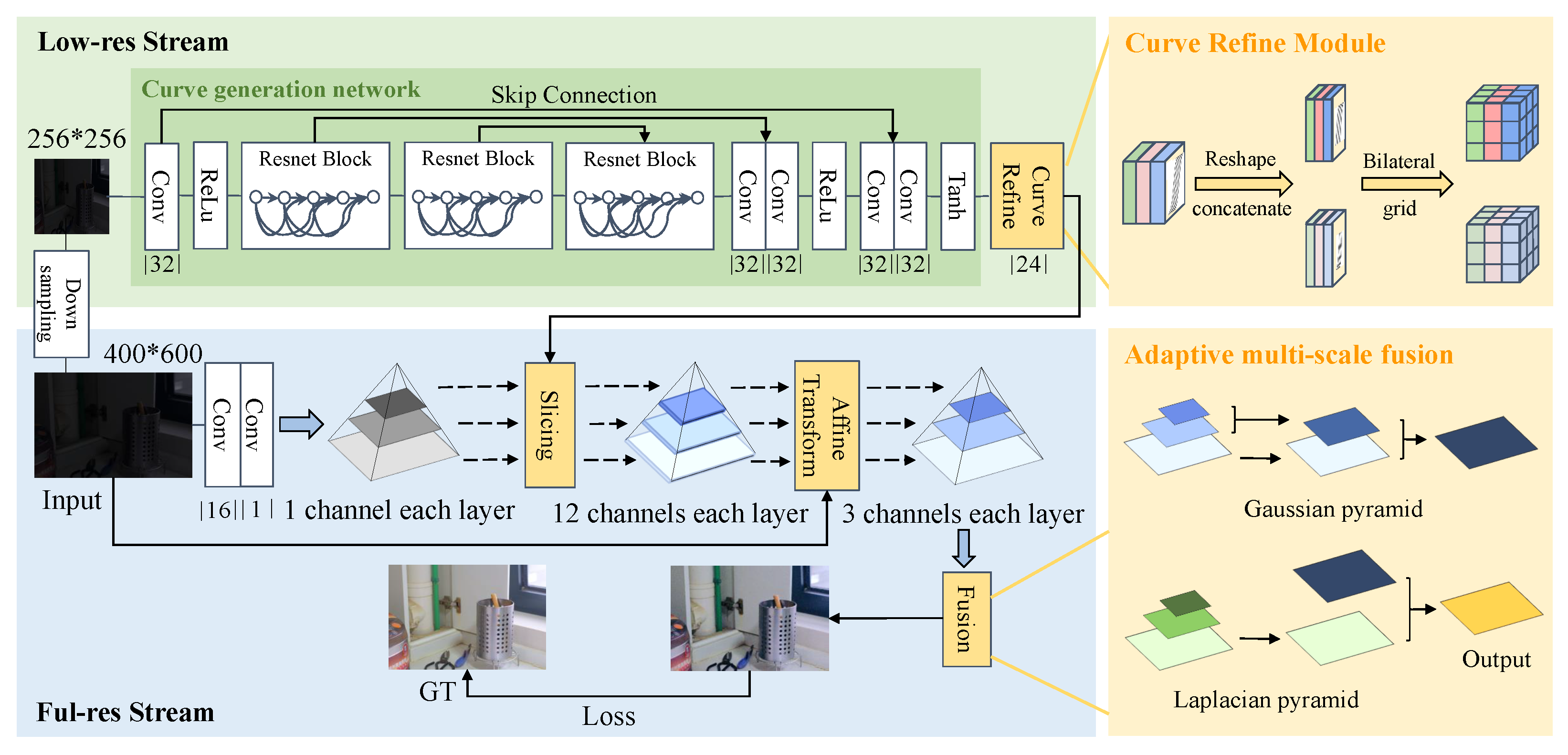
3. The Proposed Method

Figure 1 and Figure 2 respectively illustrate the overall pipeline and the specific implementation of the proposed LIMPID. Our approach is primarily composed of two branches: low-resolution stream and high-resolution stream. The former manages to learn the curve parameters corresponding to the input, while the latter transfers these parameters back to the original resolution through the guidance of grayscale maps and strengthens the color and details via image fusion.

In this section, our organization is as follows: Section 3.1 and Section 3.2 will present the background of the image-to-curve method and its implementation details in LIMPID, separately. Section 3.3 will then discuss the image fusion strategy in the full-resolution stream. Lastly, the entire information transmission and the loss functions employed will be explained in Section 3.4.

3.1. Image-to-Curve Mapping

Originally derived from the software Photoshop, the S-curve provides a tool for professional photographers to manually design adjustments to the curve so as to modify the global properties of an image, but this manner in which to retouch photographs is not universally applicable since it is relatively costly to learn for most casual users who lack artistic skills. To construct an image-to-curve mapping problem in low-light conditions, a mathematical description is introduced here that follows a similar formation of haze image generation with atmospheric light [31,32]:

$$I\left(x\right)=J\left(x\right)t\left(x\right)+A(1-t(x\left)\right),$$

(1)

where $J\left(x\right)$ is a sharp image as a target, while $t\left(x\right)$ and A are the transmittance and global atmospheric light component, respectively.

Following this model, Guo et al. [21] designed a nonlinear light enhancement curve, for which the authors iteratively estimated the image-specific curve n times to form the pixel-wise smoothing mapping function $F_c(x,y)$ in color channel c:

$$F_c^n(x,y)=F_c^{n-1}(x,y)+{\omega }_F{F}_c^{n-1}(x,y)(1-F_c^{n-1}(x,y)),$$

(2)

in which n is the number of iterations and ${\omega }_F$ denotes the curve parameter matrix.

On this basis, the proposed method further employed a more dedicated light scattering model to describe curve formation, relieving the dependence on a predefined curve shape. A low light image is expressed as the radiance arriving at the imaging plane, which is the sum of two terms at pixel X with coordinates $(x,y)$:

$$I\left(X\right)=I_d\left(X\right)+I_b\left(X\right),$$

(3)

in which $I_d$ is the direct light reflection from the objects in the scene and the $I_b$ is the scattered light. In the dehazing system [33,34,35], the clear image $J\left(X\right)$ underlies the light reflected from the target reaching the camera through particle attenuation. Modified from the direct scattering in the dehazing model with atmospheric extinction coefficient $\alpha$, $I_d$ of pixel X at $(x,y)$ in low light is:

$$I_d\left(X\right)=J\left(X\right)e^{-\alpha \left(\tau D\right(x)+D(y\left)\right)}$$

(4)

where $D\left(x\right)$ is the distance, denoting the line the light travels from a light source to the object, and $D\left(y\right)$ is the distance of the reflectance from the object to the camera. $\tau \in [0,1]$ refers to the dark attenuation coefficient to represent the virtual dark surface.

The scatted light $I_b$ is defined with the scattered distance $D\left(ry\right)$, in which r is the partition ratio of $D\left(y\right)$ to form the scatter angle $\theta$ [36], where $cos\theta =\overrightarrow{D\left(x\right)}\overrightarrow{D\left(y\right)}$. Then, its expression is:

$$I_b\left(X\right)=k{\int }_0^1\frac{e^{-a\left[\tau \right[D\left(ry\right)+1]}}{{\left[D\left(ry\right)\right]}^2}dr=kF\left(X\right)$$

(5)

where the term k is an effective constant for the absorbed radiance intensity, and $F\left(X\right)$ is the integration function of the pixel X. Especially, it is not a closed-form solution for Equation (5) in integral, but it is a smooth function with a numerical solution independent of physical parameters.

Then, according to Equation (3), we can deduce that the restored normal light image $J\left(X\right)$ is:

$$\begin{array}{c}\hfill J\left(X\right)=[I\left(X\right)-kF\left(X\right)]e^{\alpha \left(\tau D\right(x)+D(y\left)\right)}.\end{array}$$

(6)

When the term ${\omega }_{x,y}I(x,y)$ is fixed and denoted as $b_c$, the prediction of the restored image $J(x,y)$ is formed in the log domain with ${\omega }_{x,y}=\alpha (\tau D\left(x\right)+D\left(y\right))$:

$$\begin{array}{c}\hfill J(x,y)={\omega }_{x,y}(I(x,y)-k\sum _c^{}F(x,y)),\end{array}$$

(7)

$$J_c(\hat{x},y)={\omega }_c\sum _c^{}F(\hat{x},y)+b_c,$$

(8)

which represents that the restored image $J_c(\hat{x},y)$ is a linear prediction of $F_c(\hat{x},y)$ in color channels c, which is a more precise curve mapping function for the pixel-level fusion of the obtained enhanced image.

Therefore, this prediction indicates the feasibility of the proposed method to flexibly reshape the mapping curve in order to obtain a wider dynamic range in the curve refinement module, the details of which are explained in Section 3.2.

3.2. Curve Generation and Refinement

As shown in Figure 2, the backbone of our model consists of a convolutional network responsible for the image-to-curve mapping and a curve refinement module in charge of reshaping the curves into bilateral grids [23,37,38]. The convolutional network consists of three residual blocks [39] and four convolutional layers with symmetrical skip concatenation, where each convolutional layer consists of 32 convolutional kernels of size $3\times 3$ and step size 1. Each residual block consists of two such convolutional layers. The first six layers use Relu as the activation function, while the last output layer uses the tanh activation function. In our network, 24 curve mapping functions in total are produced via $n=8$ iterations, referring to the settings in [21]. As such, the output of the convolutional network is a curvilinear parametric map of 24 channels, with 8 corresponding reference curves for each pixel value for tuning.

In the curve-refinement module, the 24 mapping matrices are reshaped and concatenated into two 12-channel mapping matrices. These two grid cells are transformed into two non-overlapping up-sampled volumes in $3D$ dimensions, which formed a continuous mapping function with a broader range than single curve formation approaches.

With the help of the bilateral grid, the output of the curve-refinement module has been unrolled with a multi-channel bilateral grid, which is similar to [23], and the coordinate and luminance information is rounded and mapped inside the grid:

$$\begin{array}{c}{A}_{dc+z}{F}_c(x,y)\leftrightarrow A_c{F}_c(x,y,z),\end{array}$$

(9)

where d is the grid depth and z denotes the third dimension to represent the dynamic range. In this way, A is a $16\times 16\times 8$ bilateral grid with 2 gird cells, where each cell contains 12 digits, corresponding to the parameters in a $3\times 4$ affine matrix to achieve color channel conversion. By turning the features into bilateral grids, it allows acceleration with small resolutions. Thus, the information obtained by the low-resolution stream is stored in two grid cells, sent to the slicing layer, and transmitted back to the full-resolution version.

3.3. Adaptive Multi-Scale Fusion

Bilateral grid-based upsampling is performed on the slicing layer to scale up the low-resolution predictions to full resolution so that most of the network computations are done in the low-resolution domain, thus enabling the real-time processing of high-resolution images. However, the initial enhanced image, obtained from the output of the slicing layer after affine transformation, lacks color information, so further enhancement via image fusion is proposed. Here an extension of naive fusion is employed as our adaptive multi-scale image fusion.

As a common type of image fusion, a Gaussian pyramid is a set of pyramidal series of images with gradually decreasing resolution consisting of the same original image. Smoothing and downsampling an i-layer Gaussian pyramid can yield a $(i+1)$-layer Gaussian image:

$$G_{i+1}=Down\left(G_i\otimes G_{\mathrm{kernel}}\right),$$

(10)

where $G_{\mathrm{kernel}}$ denotes Gaussian filtering. During the dimension reduction, the original image will be convolved with a low-pass Gaussian filter matrix and then downsampled to remove even rows and columns. While in size recovery, an upsampling is performed before smoothing by the same filter.

That is, each layer is smoothed for the details of particular interest at the corresponding scale, and the smaller scale layer can approximate the results observed from a distance, which can achieve a smooth transition in grayscale when zoomed in at high resolution so that the details at different scales can be transitioned more naturally after fusion. Due to the non-linear processing of upsampling and downsampling, an irreversible information loss is generated for the image, and hence the image becomes blurred after downsampling. To solve this problem, a Laplacian pyramid is often applied to reconstruct the image by predicting the residuals at upsampling, i.e., the pixel values that need to be inserted at small-scale layer expansion, which is simply and brutally filled with zeros in the upsampling of the Gaussian pyramid. By contrast, the Laplacian pyramid fusion can predict according to the surrounding pixels, allowing for maximum restoration of the image, which can be expressed as:

$$L_i=G_i-Up\left(G_{i+1}\right)\otimes G_{\mathrm{kernel}}.$$

(11)

To perform image fusion, normally the current $(i+1)$th layer is upsampled and overlapped with the next ith layer for the ith fusion result $F_i\left(x\right)$, which can be expressed as:

$$\begin{array}{c}{F}_i\left(x\right)=G_i+\left(Up\left(F_{i+1}\left(x\right)\right)\otimes G_{\mathrm{kernel}}\right)+L_i,\\ \\ F_n\left(x\right)=G_n,\end{array}$$

(12)

where n is the total number of layers in the pyramid and $G_n$ is the smallest layer. The whole process goes from top to bottom.

Traditionally, the largest layer of the Gaussian pyramid is the standard reference image, while the Laplacian pyramid tracks the gap value between the precise image and the up-sampled blurred image. Therefore, the Gaussian pyramid and the Laplacian pyramid can turn the blurred image into a clear one when the weight of each layer is 1 (see Equation (12)). However, our largest layer, which is the output of affine transform, is an intermediate enhancement result, with difficulty to serve as a standard reference. That is to say, the ratio of colors to edges to be strengthened is not necessarily the same. To this end, the Gaussian for low-frequency information optimization and the Laplacian for high-frequency enhancement cannot simply be superimposed on the corresponding layers with the same weight.

In light of the above considerations, we divide the fusion into two steps: low-frequency information enhancement and high-frequency detail compensation. First, the color information is corrected by continuously upsampling and weighted fusion from the smallest scale layer via the Gaussian pyramid:

$$\begin{array}{c}{F}_i\left(x\right)=W_{\mathit{Gh}}{G}_i+W_{\mathit{Gl}}\left(Up\left(F_{i+1}\left(x\right)\right)\otimes G_{\mathrm{kernel}}\right),\\ \\ F_n\left(x\right)=G_n,\end{array}$$

(13)

where $W_{Gh}$ and $W_{Gl}$ denote the weights of high-resolution layers and low-resolution layers, respectively, with n as the total number of layers in the pyramid. Then, the maximum scale layer of the Laplacian pyramid is fused to compensate for the edge information:

$$L_0=G_0-Up\left(F_1\right)\otimes G_{\mathrm{kernel}}.$$

(14)

With the composition of Equations (13) and (14), a sequence of images can be generated via the following:

$$F\left(x\right)=F_0\left(x\right)+W_L{L}_0,$$

(15)

where $W_L$ represents the weight of the maximum scale layer of the Laplacian pyramid. In consideration that the optimization weight of high- and low-frequency information is not necessarily the same and the human-set parameters fail to adapt to different lighting conditions, we set a group of weight parameters ($W_{Gh}$, $W_{Gl}$, and $W_L$) that can be learned to acquire the intensity of different enhanced information, separately. By splitting the correction of color and edge information into two successive steps with learnable weights parameters, our fusion method is capable of dynamically fitting the most appropriate enhancement scheme for different inputs during model training, as shown in Figure 3.

3.4. Overall Architecture

In summary, the proposed model is divided into two branches, the full-resolution stream and the low-resolution stream. The low-resolution stream undertakes the vast majority of inference operations. The downsampled input image first proceeds through the curve generation network to learn the corresponding curve parameters. Afterward, it is reshaped into two bilateral meshes of mapped curves for a wider dynamic range during the curve refinement, which is proven reasonable in Section 3.1. Then, the full-resolution stream employs the input to construct a gray-scale Gaussian pyramid as guide maps for the slicing layer levels, leading to the upsampling of the curve parameter information based on the bilateral grids from the low-resolution stream. After that, multi-scale fusion is performed with dynamic fitting to obtain the enhanced full-resolution output.

To measure the accuracy of the recovery from the input to the enhanced image, we utilize a total loss function consisting of three loss terms, namely spatial consistency loss [21], reconstruction loss, and illumination smoothness loss [21], each with a corresponding weight, as expressed below:

$$\begin{array}{c}{L}_{total}=w_{rec}{L}_{rec}+w_{spa}{L}_{spa}+w_{tvA}{L}_{tvA},\end{array}$$

(16)

where $w_{tvA}$ is set to be 200 referring to [21]. On this basis, we found through experiments that when both A and B are 10, a higher PSNR value can be obtained as shown in Figure 4.

• Spatial consistency loss: $L_{spa}$ enhances the spatial consistency of the image by preserving the differences in adjacent regions between the enhanced image and the ground truth:

  $$L_{spa}=\frac{1}{K}\sum _{i=1}^K\sum _{j\in \Omega \left(i\right)}{\left(\mid \left(Y_i-Y_j\right)\mid -\mid \left(I_i-I_j\right)\mid \right)}^2.$$

  (17)
• Reconstruction loss: $L_{rec}$ compares the difference between the generated image and the ground truth pixel by pixel and takes the absolute value for the distance between pixels in case the positive and negative values cancel each other out.

  $$L_{rec}=\frac{1}{N}\sum _{p\in P}\mid x\left(p\right)-y\left(p\right)\mid ,$$

  (18)

  where P denotes the area of a patch, while N is the number of pixels contained within it.
• Illumination smoothness loss: $L_{tvA}$ preserves a monotonic relationship among adjacent pixels by controlling the smoothing on curve parameter matrices A:

  $$\begin{array}{c}{L}_{tvA}=\frac{1}{N}\sum _{n=1}^N\sum _c{\left(\mid {\nabla }_x{A}_n^c\mid +\mid {\nabla }_y{A}_n^c\mid \right)}^2,\\ \\ c=\{R,G,B\}.\end{array}$$

  (19)

4. Experiments

4.1. Experimental Settings

• Implementation details: Our implementation was carried out with PyTorch and trained for 2499 epochs with a mini-batch size of 6 on an NVidia GTX 1070 GPU. We used the Adam optimizer with an initial learning rate of $1e^{-3}$, and we also used the learning rate decay strategy, which reduces the learning rate to $5e^{-4}$ after 500 epochs.

To demonstrate that LIMPID can provide effective recovery of images captured in extremely low illumination, we compared it with nine SOTA methods in LLIE, including KinD++ [8], SSIENet [25], LLFlow [15], DRBN [40], EnlightenGan [41], HDRNet [23], ExCNet [18], Zero-DCE [21], and cGAN [14].

• Evaluation metrics: We choose PSNR [42], SSIM [43], GMSD [44], and FSIM [45] as objective metrics to evaluate image quality. PSNR [42] reflects the image fidelity, SSIM [43] and GMSD [44] compare the similarity of two images in terms of image structure, and FSIM compares the similarity of images in terms of luminance components.
• Datasets: The LOL-V1 dataset [6] includes 500 pairs of images taken from real scenes, each pair comprising a low-light image and a normal-light image of the same scene, with 485 pairs in the training set and 15 pairs in the testing set. The SID dataset [16] contains 5094 raw short-exposure images, each with a reference long-exposure image. The ELD dataset [17] is an extremely low-light denoising dataset composed of 240 raw image pairs in total captured over 10 indoor scenes using various camera devices. We used the training set of the LOL-V1 dataset [6] for training, and to verify the effectiveness of LIMPID, subjective and objective comparisons were made with existing SOTA methods on the testing sets of the SID dataset [16] and the ELD dataset [17].

4.2. Perceptual Comparisons

We compared the subjective results of LIMPID with the state-of-the-art. Figure 5 and Figure 6 show the test results on the ELD dataset [17] and the SID dataset [16], respectively, with the first and last images of each set being the input low-light image and the reference image, correspondingly.

As can be seen from Figure 5, DRBN [40], KinD++ [8], and SSIENet [8] are more sensitive to noise pollution, which can be proven by the presence of a large amount of noise in the black background of the noise-filled images taken in real scenes. Zero-DCE [21] and LLFlow [15] are inadequate for color and luminance enhancement, with the result being relatively darker than others. On the contrary, ExCNet [18] suffers from local over-enhancement, as Figure 5 clearly shows that ExCNet [18] enhancement results in excessive contrast. From Figure 5 and Figure 6, it appears that the results of cGan [14] are all white, lacking pixel values close to black, whereas HDRNet [23] also has a similar tendency. By contrast, the results obtained by LIMPID are minimally exposed to noise and hence there are no obvious mottled artifacts; moreover, the overall appearance after recovery from degradation is closer to the ground truth, exemplified by the overall brightness and color of the two sets of images in Figure 5.

For very dark scenes, it can be seen from Figure 6 that HDRNet [23], LLFlow [15], and KinD++ [8] have almost no enhancement effect, among which LLFlow [15] loses even the information in the original input, thus rendering it completely black, while cGan [14], EnlightenGan [41], and Zero-DCE [21] also have limited enhancement on both ends. Among the remaining methods, the results of SSIENet [25] and ExCNet [18] significantly amplify the noise, which is exhibited more severely on the noise-dense extremely low-light dataset SID [16] than on the ELD dataset [17] in Figure 5, and especially SSIENet [25] even produces green artifacts. For ExCNet [18], the enhanced result on the first image has unexpectedly clear shadows in the diffuse light on the ground as well as the streetlights, probably due to the limited dynamic range. Obviously, the proposed method and DRBN [40] have superior performance on the SID dataset [16].

It transpires that the proposed method dramatically reduces the effect of noise without a dedicated denoising module as well as providing significant color recovery for the effective enhancement of low light and even extremely low-light inputs.

4.3. Quantitative Comparisons

We compared LIMPID with several SOTA methods based on the ELD dataset [17] and the SID dataset [16], with objective results for image quality evaluation and model complexity testing shown in

Table 1. The objective image quality evaluation metrics on the SID dataset [16] and ELD dataset [17]. ↑ denotes that higher metric values represent better image quality, while for ↓ the opposite is true. Red and blue denote the best and second-best results, respectively.

Method	Datasets	SID [16]				ELD [17]
		SSIM ↑	PSNR (dB) ↑	FSIM ↑	GMSD ↓	SSIM ↑	PSNR (dB) ↑	FSIM ↑	GMSD ↓
KinD++ [8]	240 synthetic and 460 pairs in LOL-V1 [6]	0.4340	12.9617	0.6259	0.2586	0.7443	21.3444	0.7731	0.2120
SSIENet [25]	485 low-light images in LOL-V1 [6]	0.5904	17.0290	0.7301	0.2075	0.6840	18.9030	0.7923	0.1808
LLFlow [15]	LOL-V1 [6] and VE-LOL [46]	0.3835	11.8328	0.5569	0.2961	0.7034	21.7252	0.7961	0.2034
DRBN [40]	689 image pairs in LOL-V2 [29]	0.5753	17.4195	0.7483	0.2173	0.6925	19.6543	0.8116	0.2363
EnlightenGAN [41]	914 low-light and 1016 normal-light images	0.5887	16.8599	0.7321	0.2141	0.7486	21.5746	0.8244	0.1718
HDRNet [23]	485 low-light pairs in LOL-V1 [6]	0.3841	12.0539	0.5661	0.2891	0.6888	20.6590	0.8039	0.1686
ExCNet [18]	No prior training	0.5113	16.7881	0.7069	0.2416	0.6177	17.7844	0.7167	0.2369
Zero-DCE [21]	3022 multi-exposure images in SICE Part1 [47]	0.5158	15.1180	0.7265	0.2151	0.7374	19.2834	0.8317	0.1553
cGAN [14]	6559 images in LOL-V1 [6], MIT5k [48], ExDARK [49]	0.5423	15.3855	0.6676	0.2354	0.6515	17.1118	0.8018	0.1792
LIMPID	485 image pairs in LOL-V1 [6]	0.5478	17.2573	0.7383	0.2199	0.7280	23.0485	0.8239	0.1767

and

Table 2. Three objective metrics indicate the complexity of the model: parameters (in M), running time (in seconds), and FLOPs (in G), where FLOPS is the result of an input size of $256\times 256\times 3$. ‘-’ indicates the result is not available. Red and blue denote the best and second-best results, respectively.

Method	Parameters (in M) ↓	Times (s) ↓	FLOPs (G)↓
KinD++ [8]	8.275	0.392	371.27
SSIENet [25]	0.682	0.124	29.46
LLFlow [15]	17.421	0.287	286.67
DRBN [40]	0.577	2.561	28.47
EnlightenGAN [41]	8.637	0.057	16.58
HDRNet [23]	0.482	0.008	0.05
EXCNet [18]	8.274	23.280	-
Zero-DCE [21]	0.079	0.010	5.21
cGAN [14]	0.997	1.972	18.98
LIMPID	0.091	0.002	5.96

, correspondingly.

In Table 1, the PSNR of LIMPID on the SID dataset [16] and ELD dataset [17] ranks second and first, respectively, where the ELD dataset [17] is a real scene dataset containing noise, which indicates a good content similarity between our results and the ground truth and proves the validity in real scenes. By contrast, DRBN [40] and SSIENet [25], which performed well on the SID dataset [16] in terms of objective metrics, are less effective subjectively (Figure 6) and susceptible to the noise pollution, accordingly with noise in the dark amplified resulting in a more dramatic drop in performance on the ELD dataset [17], which is also verified in the subjective comparison in Section 4.1. Zero-DCE [21] achieved impressive performances on the ELD dataset [17], but its rapidly decreased expressiveness on the SID dataset [16], which shows limited generalization ability. While concordant with the findings from the subjective comparison, the metric values of KinD++ [8], HDRNet [23], and LLFlow [15] on SID [16] clearly show they are barely effective for ELLIE. In comparison, EnlightenGan [41] and the proposed LIMPID outperformed the other methods on both datasets.

Among all the compared methods, only SSIENet [25] and ExCNet [18] are zero-shot methods with only low-light images as input; by contrast, cGAN [14], EnlightenGan [41], and Zero-DCE [21] need extra normal light or multi-exposed inputs for supplementary illuminance information. The other remaining methods utilize strictly aligned paired datasets for fully-supervised training. Owing to the lack of normal illumination guidance, SSIENet [25] and ExCNet [18] appear to be unstable in performance. By contrast, our method achieves almost the same with the amount of training images being one half that of EnlightenGan [41], less than one third that of Zero-DCE [21], and even less than fifteen percent of that of cGAN [14]. As for the training efficiency shown in Table 2, most of the compared methods, including EnlightenGan [41], require far more parameters and running time than LIMPID; for example, KinD++ [8] requires 90 times more trainable parameters than LIMPID. Moreover, for the majority of indicators in Table 1, our results are superior to Zero-DCE [21], which is also a lightweight model. As shown in Table 2, our method implemented the shortest running time and the second-smallest number of trainable parameters. By downsampling the size of the input image, our method can dramatically lower the cost of FLOPs at the expense of sacrificing enhancement performance. Still, LIMPID outperformed most comparison methods. It is worth noting that the test size of FLOPs is $256\times 256\times 3$, whereas the target size of our network’s low-resolution branch is set to $256\times 256$ after downsampling the input, which means that the table cannot reflect the superiority of LIMPID. In the case of a larger input size, the FLOPs of LIMPID will be smaller than Zero-DCE [21] due to the downsampling.

To sum up, in addition to the very lightweight network structure, LIMPID can achieve very competitive performance in both perceptual and quantitative comparisons of LLIE, especially ELLIE. The proposed method enables a balance between performance and model complexity, attributed to the unique design of the curve mapping based on the light scattering model, coupled with an adaptive multi-scale fusion strategy.

4.4. Ablation Study

Experiments were performed to understand the different contributions of each module in LIMPID. Figure 7 and

Table 3. PSNR and SSIM metrics obtained in the ablation study. The values of both metrics acquired when integrating all components are optimal.

Network	Pyramid Fusion	${\mathit{L}}_{\mathit{l}1}$	${\mathit{L}}_{\mathit{spa}}$	${\mathit{L}}_{\mathit{tv}}$	PSNR (dB) ↑	SSIM ↑
	✓	✓	✓	✓	21.41	0.82
✓		✓	✓	✓	13.15	0.64
✓	✓		✓	✓	21.43	0.80
✓	✓	✓		✓	20.82	0.80
✓	✓	✓	✓		19.55	0.81
✓	✓	✓	✓	✓	21.76	0.83

show the subjective and objective performance after ablations on our sub-networks and components. For each configuration, we evaluated PSNR and SSIM metrics and validated both the significance of incorporating all modules and the superior integrated performance experimentally.

• Network Replacing our curve generation network and curve refinement module with a few superficial convolutional layers, the PSNR metric decreases by $0.3$ compared to the performance of LIMPID, and subjectively the enhancement effect is limited for relatively darker regions (see the partially enlarged area), illustrating the stability and effectiveness of our network.
• Multi-scale pyramidal fusion: With only one image as the guide map for the slicing layer and removing the subsequent image fusion, the result is significantly dimmer in color and brightness than that of LIMPID, with PSNR and SSIM reduced by about 40 percent and 20 percent, respectively, due to the dynamic enhancement of color and detail carried out by the fusion of the different scale feature maps in LIMPID.
• Loss function: The second row of Figure 7 shows the results of training through various combinations of loss functions. The absence of the L1 loss function leads to a decrease in PSNR of about $0.3$ and a more erratic appearance of color bias, indicating that the L1 loss function has a significant impact on the specification of the pixel-by-pixel similarity comparison between the input and the enhanced image. Removing the spatial consistency loss yields a result with somewhat higher contrast than the full result, as can be observed by the inconspicuous yellow color of the water pipe above the local zoom in Figure 7, along with a slight drop of about 4 percent in both PSNR and SSIM, demonstrating the importance of spatial consistency loss in preserving differences in adjacent regions of the image. Lastly, the removal of the illumination smoothing loss results in an objective decrease of $2.2$ in PSNR and a subjective decrease in the correlation between adjacent regions, thus blurring the edges, suggesting that the illumination smoothing loss preserves the monotonic relationship between adjacent pixels. Hence, it can be seen that the combination of the loss functions selected can more effectively constrain to recover the color and texture details of the image.

5. Conclusions

In this paper, we introduce image-to-curve mapping into extremely low-light image enhancement for the first time, and propose a lightweight model named LIMPID, whose performance on the restoration of color, luminance, and other degradation was validated on realistic datasets. In the proposed model, a network performs image-to-curve transformation as well as curve reshaping through an image-to-curve mapping based on the light scattering model. After that, the obtained curve is sliced in the $3D$ volume at various scale levels of the grayscale pyramid for upsampling. A dynamically adaptive multi-scale fusion strategy generates the final restored image by splitting the Gaussian and Laplacian pyramid fusion into step-wise optimization of high- and low-frequency information with learnable fusion weights.

In conclusion, we have experimentally demonstrated that LIMPID provides a solution for the ELLIE task that is applicable to real-time mobile deployment. In terms of parameter size and running time, the proposed method outperforms not only extremely low-light enhancement methods, but also other SOTA methods in LLIE.

6. Discussion

In this paper, the proposed method is primarily designed for extremely low-light scenes. With somewhat limited color and luminance information directly obtained from the extremely low-light inputs, we enlarge the number of extracted features using a pyramid fusion strategy instead of a single guide map in the full-resolution stream. However, when the proposed LIMPID is applied to cases with both over- and under-exposed regions, it is hard to achieve uniform illumination enhancement. Moreover, the over-exposed regions may be further boosted or even generate artifacts. For this real challenge of uneven illumination, we will dive into further research for solutions.

References

1. Wang, L.W.; Liu, Z.S.; Siu, W.C.; Lun, D.P. Lightening Network for Low-Light Image Enhancement. IEEE Trans. Image Process. 2020, 29, 7984–7996. [Google Scholar] [CrossRef]
2. Li, J.; Li, J.; Fang, F.; Li, F.; Zhang, G. Luminance-aware Pyramid Network for Low-light Image Enhancement. IEEE Trans. Multimed. 2020, 23, 3153–3165. [Google Scholar] [CrossRef]
3. Zhang, Y.; Zhang, J.; Guo, X. Kindling the darkness: A practical low-light image enhancer. In Proceedings of the ACMMM, Nice, France, 21–25 October 2019; pp. 1632–1640. [Google Scholar]
4. Fan, M.; Wang, W.; Yang, W.; Liu, J. Integrating semantic segmentation and retinex model for low-light image enhancement. In Proceedings of the ACMMM, Seattle, WA, USA, 12–16 October 2020; pp. 2317–2325. [Google Scholar]
5. Xu, J.; Hou, Y.; Ren, D.; Liu, L.; Zhu, F.; Yu, M.; Wang, H.; Shao, L. Star: A structure and texture aware retinex model. IEEE Trans. Image Process. 2020, 29, 5022–5037. [Google Scholar] [CrossRef] [Green Version]
6. Wei, C.; Wang, W.; Yang, W.; Liu, J. Deep retinex decomposition for low-light enhancement. arXiv 2018, arXiv:1808.04560. [Google Scholar]
7. Zhu, A.; Zhang, L.; Shen, Y.; Ma, Y.; Zhao, S.; Zhou, Y. Zero-shot restoration of underexposed images via robust retinex decomposition. In Proceedings of the ICME, London, UK, 6–10 July 2020; pp. 1–6. [Google Scholar]
8. Zhang, Y.; Guo, X.; Ma, J.; Liu, W.; Zhang, J. Beyond Brightening Low-light Images. Int. J. Comput. Vis. 2021, 129, 1013–1037. [Google Scholar] [CrossRef]
9. Atoum, Y.; Ye, M.; Ren, L.; Tai, Y.; Liu, X. Color-wise attention network for low-light image enhancement. In Proceedings of the CVPRW, Seattle, WA, USA, 14–19 June 2020; pp. 506–507. [Google Scholar]
10. Li, S.; Cheng, Q.; Zhang, J. Deep Multi-path Low-Light Image Enhancement. In Proceedings of the MIPR, Shenzhen, China, 6–8 August 2020; pp. 91–96. [Google Scholar]
11. Hu, Q.; Guo, X. Low-light Image Enhancement via Breaking Down the Darkness. arXiv 2021, arXiv:2111.15557. [Google Scholar]
12. Zhu, M.; Pan, P.; Chen, W.; Yang, Y. Eemefn: Low-light image enhancement via edge-enhanced multi-exposure fusion network. In Proceedings of the AAAI, Hilton, NY, USA, 7–12 February 2020; Volume 34, pp. 13106–13113. [Google Scholar]
13. Lv, F.; Liu, B.; Lu, F. Fast enhancement for non-uniform illumination images using light-weight CNNs. In Proceedings of the ACMMM, Seattle, WA, USA, 12–16 October 2020; pp. 1450–1458. [Google Scholar]
14. Sun, X.; Li, M.; He, T.; Fan, L. Enhance Images as You Like with Unpaired Learning. arXiv 2021, arXiv:2110.01161. [Google Scholar]
15. Wang, Y.; Wan, R.; Yang, W.; Li, H.; Chau, L.P.; Kot, A. Low-light image enhancement with normalizing flow. In Proceedings of the AAAI, Virtual, 22 February– 1 March 2022; Volume 36, pp. 2604–2612. [Google Scholar]
16. Chen, C.; Chen, Q.; Xu, J.; Koltun, V. Learning to see in the dark. In Proceedings of the CVPR, Salt Lake City, UT, USA, 18–23 June 2018; pp. 3291–3300. [Google Scholar]
17. Wei, K.; Fu, Y.; Yang, J.; Huang, H. A physics-based noise formation model for extreme low-light raw denoising. In Proceedings of the CVPR, Seattle, WA, USA, 14–19 June 2020; pp. 2758–2767. [Google Scholar]
18. Zhang, L.; Zhang, L.; Liu, X.; Shen, Y.; Zhang, S.; Zhao, S. Zero-shot restoration of back-lit images using deep internal learning. In Proceedings of the ACMMM, Nice, France, 21–25 October 2019; pp. 1623–1631. [Google Scholar]
19. Moran, S.; Marza, P.; McDonagh, S.; Parisot, S.; Slabaugh, G. Deeplpf: Deep local parametric filters for image enhancement. In Proceedings of the CVPR, Seattle, WA, USA, 14–19 June 2020; pp. 12826–12835. [Google Scholar]
20. Moran, S.; McDonagh, S.; Slabaugh, G. Curl: Neural curve layers for global image enhancement. In Proceedings of the ICPR, IEEE, Milan, Italy, 10–15 January 2021; pp. 9796–9803. [Google Scholar]
21. Guo, C.; Li, C.; Guo, J.; Loy, C.C.; Hou, J.; Kwong, S.; Cong, R. Zero-reference deep curve estimation for low-light image enhancement. In Proceedings of the CVPR, Seattle, WA, USA, 14–19 June 2020; pp. 1780–1789. [Google Scholar]
22. Li, C.; Guo, C.; Ai, Q.; Zhou, S.; Loy, C.C. Flexible Piecewise Curves Estimation for Photo Enhancement. arXiv 2020, arXiv:2010.13412. [Google Scholar]
23. Gharbi, M.; Chen, J.; Barron, J.T.; Hasinoff, S.W.; Durand, F. Deep Bilateral Learning for Real-Time Image Enhancement. ACM Trans. Graph. 2017, 36, 118. [Google Scholar] [CrossRef]
24. Jobson, D.J.; Rahman, Z.u.; Woodell, G.A. A multiscale retinex for bridging the gap between color images and the human observation of scenes. IEEE Trans. Image Process. 1997, 6, 965–976. [Google Scholar] [CrossRef] [Green Version]
25. Zhang, Y.; Di, X.; Zhang, B.; Wang, C. Self-supervised image enhancement network: Training with low light images only. arXiv 2020, arXiv:2002.11300. [Google Scholar]
26. Wang, Y.; Cao, Y.; Zha, Z.J.; Zhang, J.; Xiong, Z.; Zhang, W.; Wu, F. Progressive retinex: Mutually reinforced illumination-noise perception network for low-light image enhancement. In Proceedings of the ACMMM, Nice, France, 21–25 October 2019; pp. 2015–2023. [Google Scholar]
27. Ren, X.; Yang, W.; Cheng, W.H.; Liu, J. Lr3m: Robust low-light enhancement via low-rank regularized retinex model. IEEE Trans. Image Process. 2020, 29, 5862–5876. [Google Scholar] [CrossRef]
28. Hao, S.; Han, X.; Guo, Y.; Xu, X.; Wang, M. Low-light image enhancement with semi-decoupled decomposition. IEEE Trans. Multimed. 2020, 22, 3025–3038. [Google Scholar] [CrossRef]
29. Yang, W.; Wang, W.; Huang, H.; Wang, S.; Liu, J. Sparse gradient regularized deep retinex network for robust low-light image enhancement. IEEE Trans. Image Process. 2021, 30, 2072–2086. [Google Scholar] [CrossRef]
30. Hai, J.; Xuan, Z.; Yang, R.; Hao, Y.; Zou, F.; Lin, F.; Han, S. R2RNet: Low-light Image Enhancement via Real-low to Real-normal Network. arXiv 2021, arXiv:2106.14501. [Google Scholar] [CrossRef]
31. McCartney, E.J. Optics of the atmosphere: Scattering by molecules and particles. New York 1976. Available online: https://ui.adsabs.harvard.edu/abs/1976nyjw.book.....M/abstract (accessed on 1 March 2023).
32. Nayar, S.K.; Narasimhan, S.G. Vision in bad weather. In Proceedings of the Seventh IEEE International Conference on Computer Vision, IEEE, Corfu, Greece, 20–27 September 1999; Volume 2, pp. 820–827. [Google Scholar]
33. Sun, B.; Ramamoorthi, R.; Narasimhan, S.; Nayar, S. A practical analytic single scattering model for real time rendering. ACM Trans. Graph. 2005, 24, 1040–1049. [Google Scholar] [CrossRef] [Green Version]
34. Narasimhan, S.G.; Gupta, M.; Donner, C.; Ramamoorthi, R.; Nayar, S.K.; Jensen, H.W. Acquiring Scattering Properties of Participating Media by Dilution. ACM Trans. Graph. 2006, 25, 1003–1012. [Google Scholar] [CrossRef]
35. Guo, X.; Yu, L.; Ling, H. LIME: Low-light Image Enhancement via Illumination Map Estimation. IEEE Trans. Image Process. 2016, 26, 983–993. [Google Scholar] [CrossRef]
36. Tsiotsios, C.; Angelopoulou, M.E.; Kim, T.K.; Davison, A.J. Backscatter Compensated Photometric Stereo with 3 Sources. In Proceedings of the CVPR, Columbus, OH, USA, 23–28 June 2014; pp. 2259–2266. [Google Scholar] [CrossRef] [Green Version]
37. Paris, S.; Durand, F. A fast approximation of the bilateral filter using a signal processing approach. In Proceedings of the ECCV, Graz, Austria, 7–13 May 2006; Springer: Berlin/Heidelberg, Germany, 2006; pp. 568–580. [Google Scholar]
38. Chen, J.; Paris, S.; Durand, F. Real-time edge-aware image processing with the bilateral grid. ACM Trans. Graph. 2007, 26, 103-es. [Google Scholar] [CrossRef]
39. He, K.; Zhang, X.; Ren, S.; Sun, J. Deep residual learning for image recognition. In Proceedings of the CVPR, Las Vegas, NV, USA, 27–30 June 2016; pp. 770–778. [Google Scholar]
40. Yang, W.; Wang, S.; Fang, Y.; Wang, Y.; Liu, J. Band representation-based semi-supervised low-light image enhancement: Bridging the gap between signal fidelity and perceptual quality. IEEE Trans. Image Process. 2021, 30, 3461–3473. [Google Scholar] [CrossRef]
41. Jiang, Y.; Gong, X.; Liu, D.; Cheng, Y.; Fang, C.; Shen, X.; Yang, J.; Zhou, P.; Wang, Z. Enlightengan: Deep light enhancement without paired supervision. IEEE Trans. Image Process. 2021, 30, 2340–2349. [Google Scholar] [CrossRef] [PubMed]
42. Hore, A.; Ziou, D. Image quality metrics: PSNR vs. SSIM. In Proceedings of the ICPR, IEEE, Istanbul, Turkey, 23–26 August 2010; pp. 2366–2369. [Google Scholar]
43. Wang, Z.; Bovik, A.C.; Sheikh, H.R.; Simoncelli, E.P. Image quality assessment: From error visibility to structural similarity. IEEE Trans. Image Process. 2004, 13, 600–612. [Google Scholar] [CrossRef] [PubMed] [Green Version]
44. Xue, W.; Zhang, L.; Mou, X.; Bovik, A.C. Gradient Magnitude Similarity Deviation: A Highly Efficient Perceptual Image Quality Index. IEEE Trans. Image Process. 2014, 23, 684–695. [Google Scholar] [CrossRef] [Green Version]
45. Zhang, L.; Zhang, L.; Mou, X.; Zhang, D. FSIM: A Feature Similarity Index for Image Quality Assessment. IEEE Trans. Image Process. 2011, 20, 2378–2386. [Google Scholar] [CrossRef] [Green Version]
46. Liu, J.; Xu, D.; Yang, W.; Fan, M.; Huang, H. Benchmarking low-light image enhancement and beyond. Int. J. Comput. Vis. 2021, 129, 1153–1184. [Google Scholar] [CrossRef]
47. Cai, J.; Gu, S.; Zhang, L. Learning a deep single image contrast enhancer from multi-exposure images. IEEE Trans. Image Process. 2018, 27, 2049–2062. [Google Scholar] [CrossRef]
48. Bychkovsky, V.; Paris, S.; Chan, E.; Durand, F. Learning photographic global tonal adjustment with a database of input/output image pairs. In Proceedings of the CVPR 2011, IEEE, Colorado Springs, CO, USA, 20–25 June 2011; pp. 97–104. [Google Scholar]
49. Loh, Y.P.; Chan, C.S. Getting to know low-light images with the exclusively dark dataset. Comput. Vis. Image Underst. 2019, 178, 30–42. [Google Scholar] [CrossRef] [Green Version]
Figure 1. Flow chart of the proposed LIMPID.
Photonics 10 00273 g001
Figure 2. Overall framework of LIMPID consists of two streams. The low-resolution stream maps the downsampled input to image-specific curves with parameter information stored in two bilateral grid volumes. Then, the full-resolution stream constructs a gray-scale Gaussian pyramid as a guide map for slicing, and upsamples the curve parameter information to full resolution. Finally, the full-resolution output is obtained after boosting the color and texture with adaptive multi-scale fusion.
Photonics 10 00273 g002
Figure 3. Comparison of subjective results with different fusion strategies, with non-dynamic and dynamic results respectively corresponding to Equations (12) and (15).
Photonics 10 00273 g003
Figure 4. The PSNR values corresponding to the varying weights of the spatial consistency loss and reconstruction loss. The x and y axes respectively represent w s p a and w r e c , with the number in a bubble being the PSNR value (dB), whose magnitudes are positively correlated with the square size of its bubble.
Photonics 10 00273 g004
Figure 5. Results on the ELD dataset of LIMPID and existing SOTA methods in LLIE.
Photonics 10 00273 g005
Figure 6. Results on the SID dataset of LIMPID and existing SOTA methods in LLIE.
Photonics 10 00273 g006
Figure 7. Subjective results of ablation studies on different modules. Comparing the recovered tones and brightness, the enhanced outcome obtained by LIMPID is closer to the ground truth overall.
Photonics 10 00273 g007