Article

Optical Bottle Shaping Using Axicons with Amplitude or Phase Apodization

by
Svetlana N. Khonina
1,2,*,
Andrey V. Ustinov
2,
Sergey I. Kharitonov
1,2,
Sergey A. Fomchenkov
1,2 and
Alexey P. Porfirev
1,2
1
Samara National Research University, Samara 443086, Russia
2
Image Processing Systems Institute of RAS—Branch of the FSRC “Crystallography and Photonics” RAS, Samara 443001, Russia
*
Author to whom correspondence should be addressed.
Photonics 2023, 10(2), 200; https://doi.org/10.3390/photonics10020200
Submission received: 11 January 2023 / Revised: 4 February 2023 / Accepted: 7 February 2023 / Published: 13 February 2023

Abstract

:
We investigate the formation of single and multiple optical bottle beams on the optical axis using a diffractive axicon with amplitude or phase apodization. The proposed approach allows one to control the location and the contrast of the boundaries of the generated dark intensity regions on the optical axis. Experimental results obtained using a spatial light modulator are in good agreement with numerically obtained ones. We successfully used the designed and experimentally formed set of three optical bottle beams for trapping light-absorbing agglomerations of carbon nanoparticles in air under the action of photophoretic forces. This confirms the efficiency of the proposed approach for optical manipulation applications.

1. Introduction

Demonstration in 1986 of single-beam optical tweezers that use only a single strongly focused beam for trapping and manipulation of nano- and micro-objects [1] led to the rapid involvement of laser manipulation techniques in various fields of biology [2], medicine [3], chemistry [4], and physics [5,6]. Optical tweezers made it possible to carry out unique measurements of the viscoelastic properties of single DNA molecules [7], to trap an erythrocyte in the capillary of a living mouse [8], and to cool atoms to ultra-low temperatures [9]. Further development of the optical tweezers technique led to the creation of the so-called holographic optical tweezers (HOTs) [10,11]. HOTs made it possible to further expand the functionality of the laser manipulation technique because of the use of the so-called structured laser beams [12], laser fields with a complex distribution of amplitude, phase, and/or polarization. One of the most widely used types of HOTs is the so-called optical bottle beam, an optical beam with a minimal or zero intensity region three-dimensionally surrounded by regions of higher intensity [12,13,14,15]. The optical bottle beams are widely used for the realization of stable trapping and three-dimensional guiding of the trapped particles [16,17]. Especially this type of optical trap is useful for light-absorbing particles [18] as well as for atoms [19] and low-index and opaque particles [20], which are pushed out of areas of high intensity (that is why it is necessary to form a dark area surrounded by a light barrier). There are various approaches to the shaping of optical bottle beams. One of the simplest solutions is the interference of two Laguerre-Gaussian (LG) beams resulting in the generation of a dark focal area surrounded in all directions by regions of higher intensity. In Ref. [13], such LG beams superposition was generated using an amplitude hologram which is characterized by low diffraction efficiency. Hollow Gaussian beams [21] generated by the transformation of an LG beam using a spiral phase plate [22], by spatial filtering [23], or by thermal lens effect [24] also allow one to generate a single optical bottle beam. The shadow focus can also be formed by inserting a π-phase shift in the central part of the focused Gaussian beam regarding the periphery [25,26,27]. However, the intensity of the “walls” of such a trap is quite low. To solve this problem, beams with auto-focusing properties can be used [28,29,30]. The caustics of auto-focusing beams provide a sufficiently high intensity of the bottle walls.
Another method of optical bottle beam generation is applying superimposed optical vortex beams [17]. This approach provides the photophoresis-based optical manipulation of light-absorbing particles. However, the shaped optical traps have a phase singularity on the optical axis. Therefore, the formed intensity minimum is not surrounded by the light walls in all directions. Such bottles are suitable only for trapping particles whose dimensions correspond to the size of the central region of the formed trap. The same problem is typical for the optical bottle beams generated using a binary phase mask and a focusing lens illuminated by a radially or azimuthally polarized laser beam [31]. Single vector optical bottle beams with spatially variant light polarization can be formed from a single Gaussian beam by passing it through a uniaxial crystal [32].
It is also possible to define the desired three-dimensional (3D) light field distribution near the optical axis and design a special diffractive or holographic optical element, for example, by an iterative method [33,34,35]. In particular, a numerical procedure based on a modified genetic algorithm was used for optimizing a binary phase element generating an optical bottle with definite intensity distribution [36]. Later, this element was experimentally studied [37]. More exotic techniques, such as conical refraction of light in a biaxial crystal [38] and Moiré techniques [39], also allow one to create single optical bottle beams.
Sometimes, a tandem of two optical elements, a lens, and an axicon, is used to shape optical bottle beams [19,40,41,42,43,44,45]. In this case, the dark region of the intensity is formed in the focal plane of the lens. The parameters of the generated optical trap can be dynamically changed both because of the characteristics of the axicon [44,45] and by changing the distance between these two elements [41]. However, as a rule, the optical bottle formed by this method has a large transverse size, which prevents the stable capture of a single particle.
Note the most considered approaches are focused on the formation of single optical bottle beams. The generation of multiple optical bottle beams spatially separated in the plane, which is transverse to the optical axis, was investigated in several works [20,45,46]. Moreover, as a rule, the position of the dark regions on the optical axis is also rigidly defined—it is not possible to shift the position of one trap relative to others.
It is well known that an axicon [47,48] generates an extended axial distribution corresponding to the Bessel beam [49,50]. The self-healing features of the Bessel beam are very useful when trapping many transparent particles along the optical axis [51]. However, to trap many opaque particles, we need to create many axial bottles.
In this paper, we consider an easy-to-implement approach for the formation and control of a set of optical bottle beams on the optical axis. This approach can be implemented by applying amplitude or phase apodization of the fabricated axicon or using a spatial light modulator (SLM) to generate the calculated phase function. There are various studies where amplitude or phase apodization of axicons is used. In particular, the illumination of an axicon by a diverging Gaussian beam makes it possible to form a scale-varying Bessel beam [52,53]. In addition, the diaphragming apertures control the uniformity of intensity and the longitudinal size of the formed light axial segment [54]. Phase apodization of a conical axicon by an additional annular grating was used in [55] to reduce the transverse size of the light line. However, these works did not investigate the formation of axial optical bottles.
Note the use of fractal [56,57,58,59] and binary [60,61] optical elements makes it possible to form many local foci at certain positions along the optical axis. To vary the axial positions, more complex optical elements are used, which are a superposition of different focusing wavefronts [62,63]. In this paper, we consider a simpler approach based on amplitude or phase apodization of a conventional axicon and investigate the effectiveness of various types of apodization. Such an approach has all the advantages of using conventional axicons and the possibility to control not only the number of traps formed but also their relative position, which is important for solving problems of optical manipulation.

2. Theoretical Foundations and Modeling

The complex transmission function of a diffractive axicon that collects incident radiation on the optical axis is described as follows:
τ a x ( r ) = exp i k α r ,
where k = 2π/λ is the wavenumber of incident laser radiation with the wavelength λ and α is the axicon parameter corresponding to the numerical aperture.
In the paraxial case, when α << 1, it is possible to calculate the diffraction of the incident axisymmetric field A(r) at the axicon defined by Equation (1) using the Hankel-Fresnel transformation:
G ( ρ , z ) = i k z exp ( i k z ) exp i k ρ 2 2 z 0 g ( r ) exp i k r 2 2 z J 0 k r ρ z r d r
where g(r) = A(rax(r), z is the distance from the input plane, J0(x) is the zero-order Bessel function of the first kind.
Analytical calculation of the integral defined by Equation (2) is problematic in most cases, but for a region not very close to the optical axis, an approximate expression can be obtained. In particular, in [64], Equation (2) is reduced to the following form:
G ( ρ , z ) e i π / 4 exp ( i k z ) exp i k ρ 2 2 z k 2 π ρ z 0 g ( r ) exp i k r 2 2 z exp i k r ρ z r d r
Note, Equation (3), unlike Equation (2), allows the use of the stationary phase method. This makes it possible to obtain an approximate expression for the integral in Equation (3) for specific types of function g(r).
In this paper, we are mainly interested in the distribution on the optical axis (ρ = 0). In this case, Equation (2) is simplified and reduced to the following form:
G ( 0 , z ) = i k z exp ( i k z ) 0 g ( r ) exp i k r 2 2 z r d r
However, these works did not investigate the formation of a set of axial optical bottles. In this paper, we investigate the possibility of forming a set of axial optical bottles using a simple approach based on the amplitude or phase apodization of a conventional axicon. We analyze the effectiveness of different types of apodization in the following sections.

2.1. Axial Distribution Control by Amplitude Apodization of the Axicon

Amplitude apodization seems to us the easiest to implement since it can be implemented by changing the parameters of the illuminating beam or by simple diaphragming [52,53,54]. Before solving the main task of forming a set of axial optical bottles, we study the effect of axicon diaphragming on the axial distribution in detail.

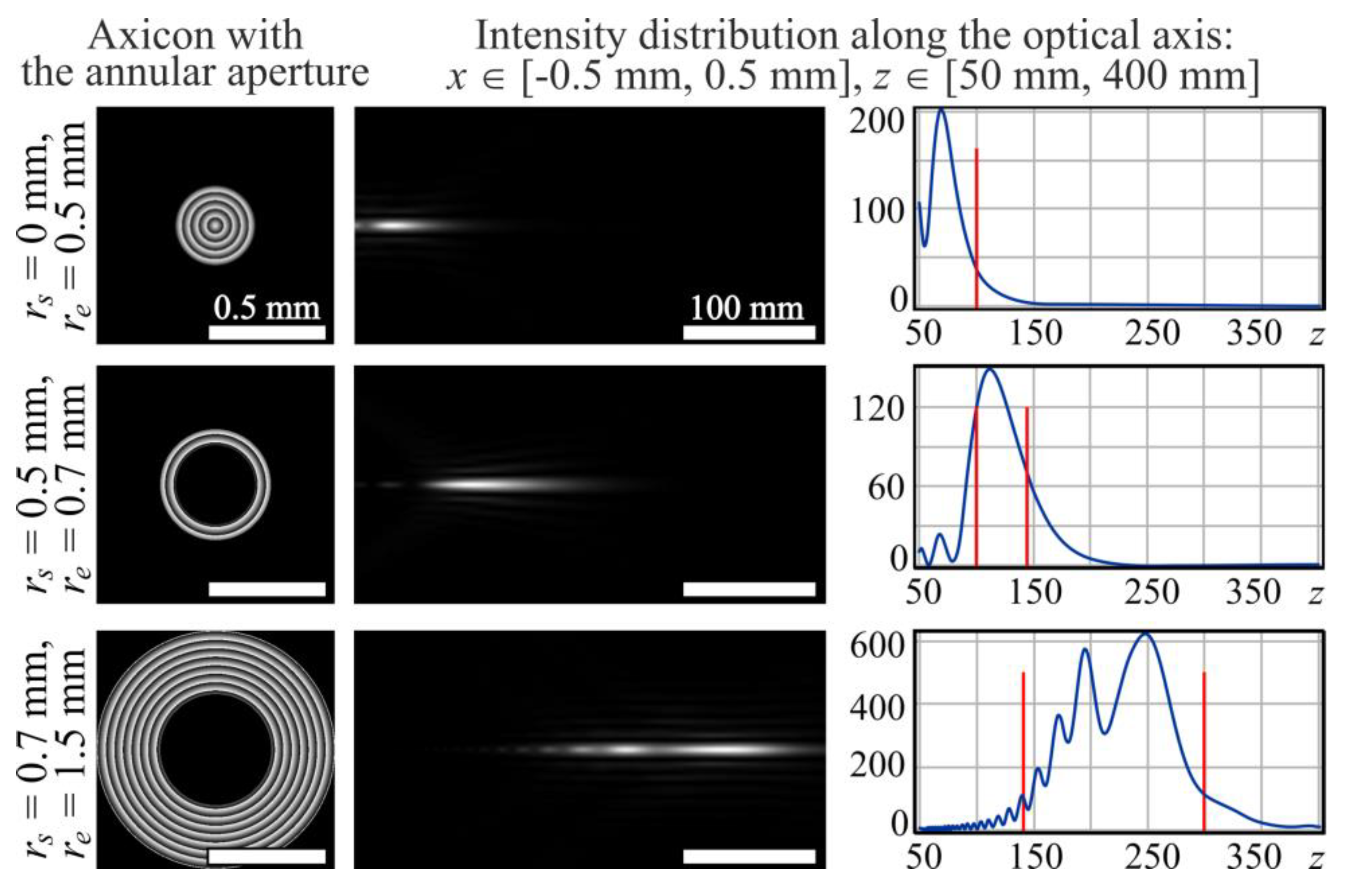
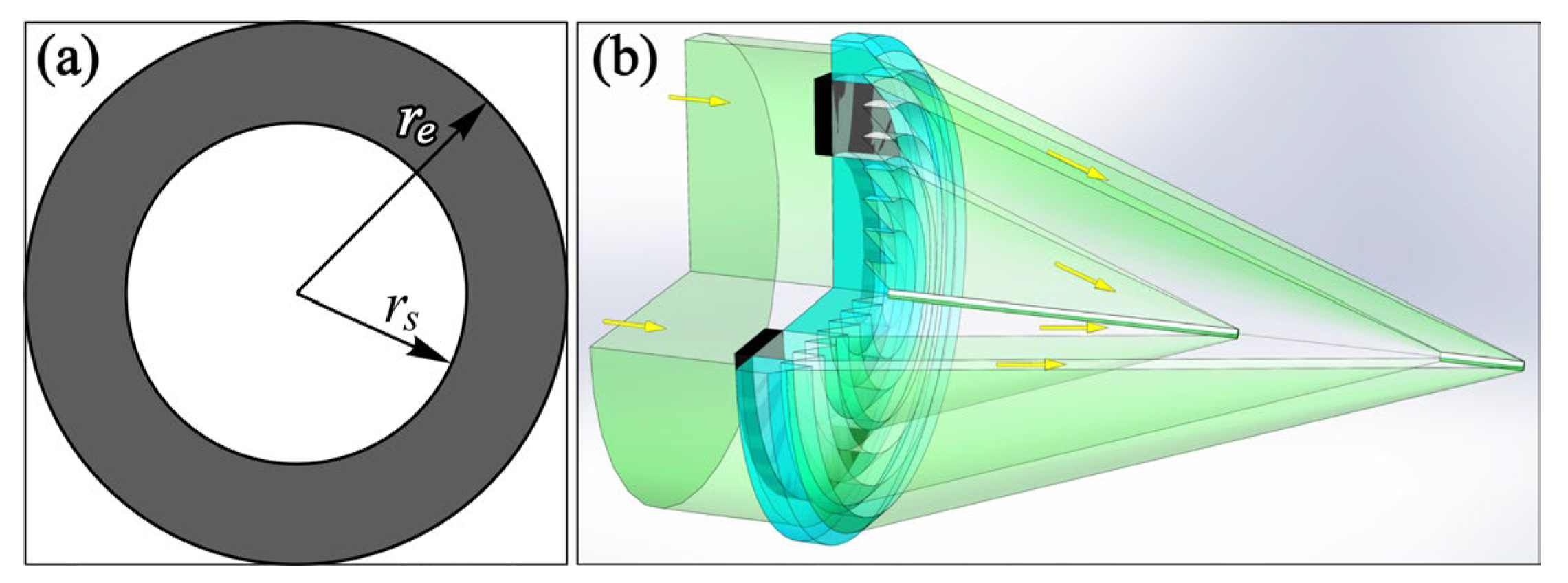
2.1.1. Formation of an Axial Light Segment Using an Annular Slot

Let us consider the incident radiation A(r) corresponding to a plane wave bounded by an annular slot (diaphragm) of the following form:
A r n g ( r ) = 1 , r s r r e , 0 , else .
where rs and re are the inner and outer radii of the annular slot (see Figure 1).
For an axicon bounded by an annular slot grax(r) = Arng(rax(r), Equation (4) for the distribution on the optical axis will take the following form:
G r a x ( 0 , z ) = i k z exp ( i k z ) r s r e exp ( i k α r ) exp i k r 2 2 z r d r
Applying the classical method of the stationary phase [65], we obtain the following explicit approximate expression [66]:
G r a x ( 0 , z ) e i π / 4 α 2 π k z exp i k z 1 α 2 2 , r s / α z r e / α , 0 , else .
The intensity distribution on the optical axis is given by a simple expression:
I r a x ( 0 , z ) 2 π k z α 2 , r s / α z r e / α , 0 , else .
Equation (8), obtained using the stationary phase method, corresponds to the geometric-optical approach. In a geometric approximation, the rays passing through the optical element on the ring with radius r will be focused on the optical axis at a distance z = r/α. Thus, the annular aperture defined by Equation (5) should ensure the formation of an axial light segment in the range zs = rs/α ≤ zze = re/α. Note that the length of the axial light segment and its position is determined only by the axicon parameter α and the boundaries of the annular aperture rs, re. Obviously, the use of several annular apertures makes it possible to form a chain of light segments with a certain length and position. This approach can also be used to form optical traps.
Note, however, that the simple geometric-optical approach described above is an approximation. Figure 2 shows the simulation results with the calculation of the integral in Equation (2) by the method of numerical integration for an axicon of Equation (1) with α = 0.005, illuminated by a flat annular beam of various sizes with a wavelength of λ = 532 nm. The red vertical lines on the intensity plots (third column of Figure 2) correspond to the geometric boundaries zs = rs/α, ze = re/α.
As can be seen from the results shown in Figure 2, the geometric-optical boundaries of the light segments are rather approximate (part of the energy is outside, or vice versa, does not completely fill the interval) due to diffraction effects. However, in general, the use of an annular aperture makes it quite simple and effective to vary the length and position of the formed axial light segments.
Let’s consider a more precise description of the formed axial light segment using an axicon. The integral in Equation (6) within arbitrary limits is equal to:
r 1 r 2 exp ( i k α r ) exp i k r 2 2 z r d r = T 1 + T 2
T 1 = z i k exp i k r 2 2 z i k α r r 1 r 2 , T 2 = α z λ z 2 exp i k α 2 z / 2 ± E t 2 E t 1 ,
where t i = k 2 z r i α z 2 , E x = C ( x ) + i S ( x ) , C ( x ) S ( x ) = 1 2 π 0 x 1 t cos ( t ) sin ( t ) d t are the Fresnel functions.
In the last line of Equation (10), the upper sign is placed if the expression (ri − αz) is positive and the lower sign otherwise.
It can be seen from Equations (9) and (10) that the distribution on the axial light segment has an oscillating character and does not have a clear cutoff boundary. Similar expressions were analyzed in [66], where it was shown that the terms containing the Fresnel functions “on average” are larger than the other terms.

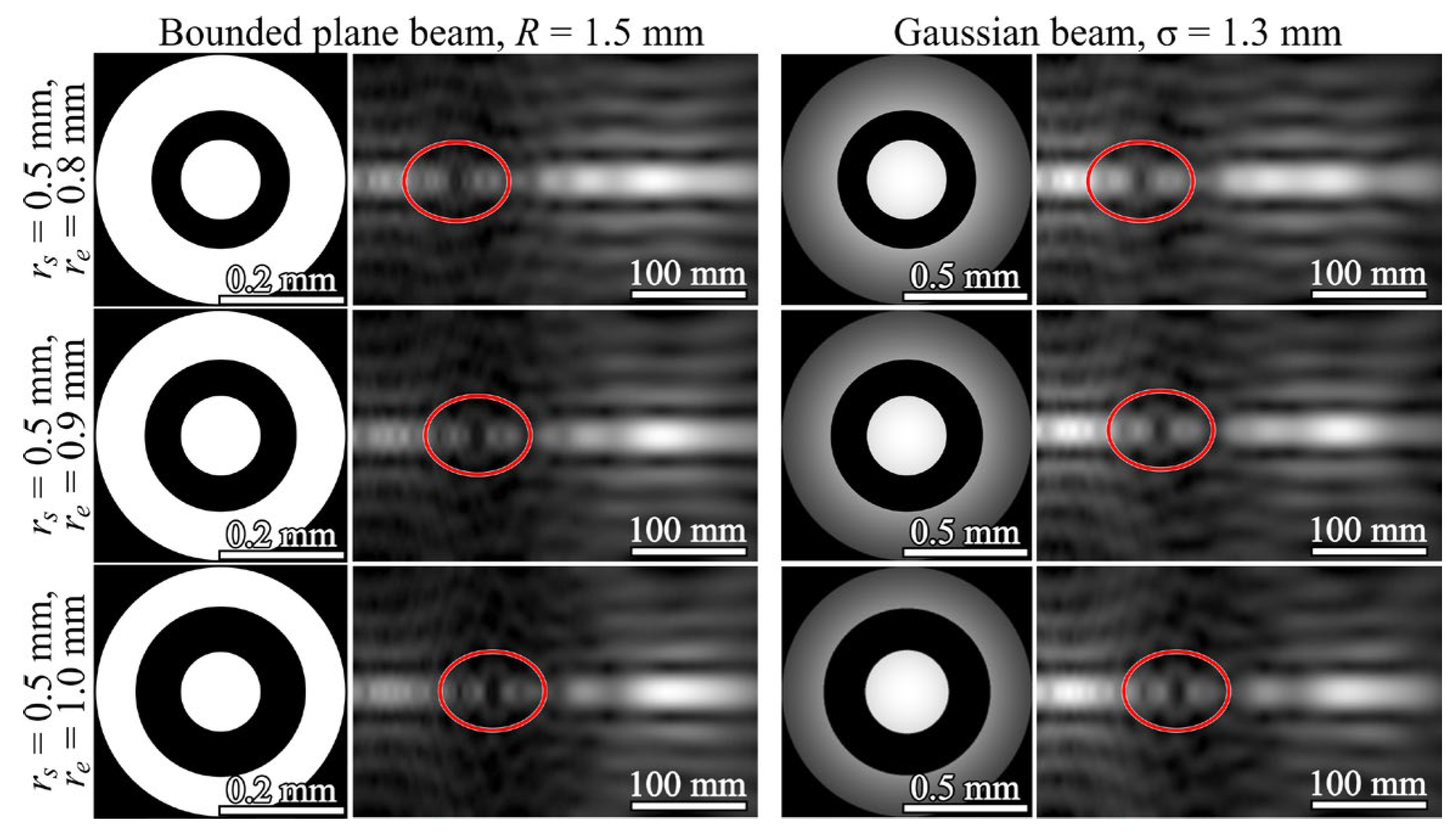
2.1.2. Formation of an Optical Bottle when Applying an Annular Blocking Screen

Although the geometric model of the axicon action is approximate, the considered properties of the axicon can be quite simply used to form an optical bottle due to the blocking of radiation by an annular screen. In this case, the illuminating beam will have the following form:
A b l ( r ) = 0 , r s r r e , A ( r ) , else .
where rs and re are the inner and outer radii of the annular blocking screen (see Figure 3a).
Figure 3 shows a geometric-optical illustration of the formation of an optical bottle due to the blocking of radiation by an annular screen. In this case, rays from the central and peripheral parts of the axicon form the neck and bottom of the bottle, and the bottle cavity is formed on the segment of the optical axis corresponding to the blocking ring.
The field on the optical axis when the axicon is blocked by an annular screen gblax(r) = Abl(rax(r) is described by the following expression:
G b l a x ( 0 , z ) = i k z exp ( i k z ) × × 0 r s exp ( i k α r ) exp i k r 2 2 z r d r + r e R exp ( i k α r ) exp i k r 2 2 z r d r .
To correctly describe the properties of the bottle formed by blocking the axicon with an annular screen, we calculate the amplitude on the axis using Equations (9) and (10):
G b l a x ( 0 , z ) = ( 1 ) exp ( i k z ) exp i k r s 2 2 z i k α r s 1 + + i π α k z exp i k z 1 α 2 2 ± E k 2 z r s α z 2 E k 2 z 0 α z 2 + + ( 1 ) exp ( i k z ) exp i k R 2 2 z i k α R exp i k r e 2 2 z i k α r e + + i π α k z exp i k z 1 α 2 2 ± E k 2 z R α z 2 E k 2 z r e α z 2 .
Let us consider in detail the behavior of the amplitude in the region, which is a geometric shadow: rs/α ≤ zre/α. In this area, taking into account the analysis performed in [66], we will take into account only terms with the Fresnel functions. Since the factors in front of the curly brackets in Equation (13) are the same, we can look at the behavior of the values inside these brackets.
In the first term (corresponds to a circle 0 ≤ rrs) in the shadow area rs < αz (obviously, 0 < αz) and it is necessary to take the lower signs; so let’s analyze the expression {E[(k/2)α2z] − E[(k/2)(αz − rs)2]}. The first term, E[·], is a large number, so we can replace the Fresnel functions with limit values ½. Thus, we analyze the function:
1 2 + i 2 C k 2 z ( α z r s ) 2 i S k 2 z ( α z r s ) 2
The field intensity in Equation (13) is proportional to the square of the modulus of Equation (14). Using tables, we can see that ((1/2) − C(x))2 + (1/2) − S(x))2 decreases as x increases. Applying the asymptotic formulas with two terms, we obtain that the sum of squares is equal to (2πx)−1. The decrease is monotonous, and there is no characteristic point. Therefore, we conditionally take the value z corresponding to x = μ as the left border of the shadow (μ depends on the selected fall level). Solving the quadratic equation kz − rs)2/2z = μ, we find the root lies in the shadow area (z > rs/α):
z s = ( k α r s + μ ) + μ 2 + 2 μ k α r s k α 2 r s α + 2 μ k α r s k α 2
Similarly, in the second term (corresponds to the ring rerR) in the region of the shadow re > αz (R > αz) and it is necessary to take the upper signs, so we analyze the expression {E[(k/2z)(R − αz)2] − E[(k/2z)(re αz)2]}. The first term, E[·], is a large number, so this expression is reduced to
1 2 + i 2 C k 2 z ( r e α z ) 2 i S k 2 z ( r e α z ) 2
which is similar to Equation (14). The right boundary of the shadow is found by a formula similar to Equation (15) (taking into account the root in the shadow region, i.e., z < re/α):
z e = ( k α r e + μ ) μ 2 + 2 μ k α r e k α 2 r e α 2 μ k α r e k α 2
Finally, the shadow region does not have sharp boundaries and is narrower compared to the geometric-optical interval due to the overlap of the “tails” from the illuminated parts of the axicon:
z s r s α + 2 μ k α r s k α 2 < z < z e r e α 2 μ k α r e k α 2
where μ is the chosen level of tail fall.
Figure 4 shows the results of the simulation using Equation (2) by the method of numerical integration for the axicon defined by Equation (1) with α = 0.005, illuminated by a flat beam, limited by radius R = 1.5 mm, with a wavelength λ = 532 nm. Ring screen radii are rs = 0.5 mm and re = 0.7 mm.
As can be seen from Figure 4, the numerical result corresponds to the above theoretical reasoning, i.e., there is an illumination of the shadow area due to the overlap of the “tails” from the illuminated parts of the axicon.
Note that using a Gaussian illumination beam A(r) = exp(−r22) instead of a flat beam (see Figure 5) can equalize the intensity values at the beginning and the end of the light bottle, but in this case, the shadow area becomes even worse.
The light walls of the cavity outside the optical axis are formed due to diffraction effects (see Figure 4 and Figure 5).
To improve the quality of the formed trap, one can increase the width of the blocking ring. To avoid overlap in the shadow area, it needs to be zs < ze. Using the approximate Equation (18), we transform this condition into the inequality:
r e r s > 2 μ k α
For the assigned inner border rs of the blocking screen, one can define the outer border re using the following convenient expression:
r e r s > 2 μ k α + 2 2 μ r s k α
Figure 6 shows the results of a comparative simulation of the light bottle formation due to radiation blocking by an annular screen under illumination with a bounded flat and the Gaussian beam.
It can be seen from the simulation results (Figure 6) that illumination with the Gaussian beam provides a more pronounced formation of an optical trap due to the smoothness of the field. Note, despite the increase in the width of the blocking ring, the longitudinal size of the hollow part of the trap increases slightly, although it moves further from the optical element as expected.

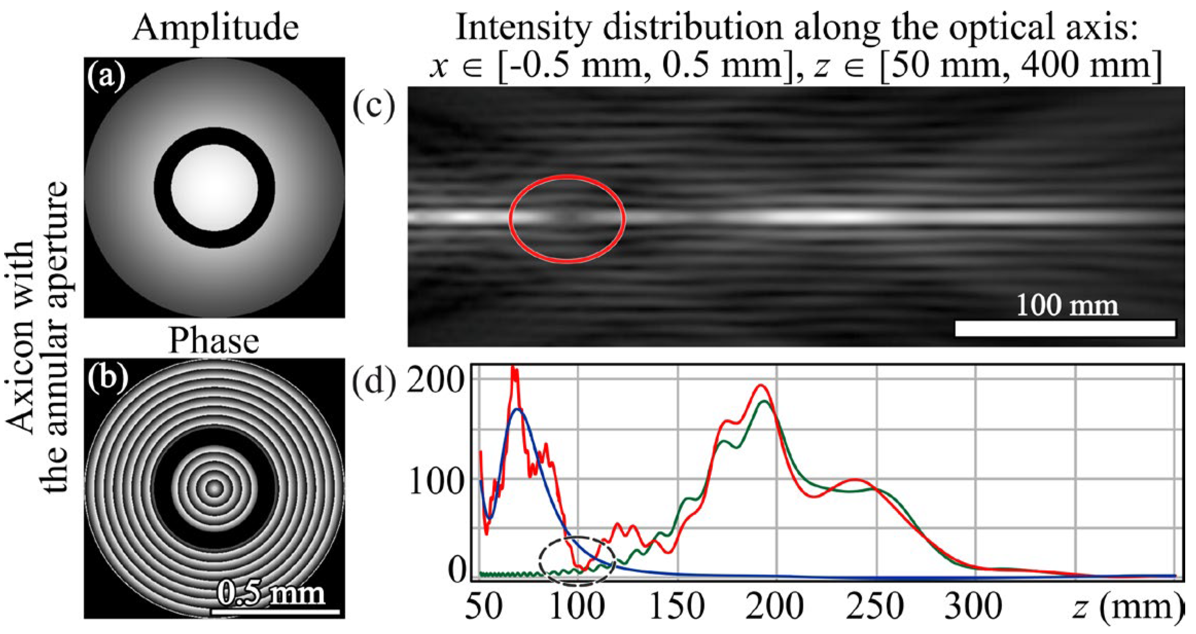
2.2. Formation of Optical Bottles by Phase Apodization of Axicons

Phase apodization of a fabricated axicon is more difficult to implement since it requires the use of an additional phase element. However, phase apodization can be taken into account when calculating a composite element and optimized using SLM. In addition, phase apodization is more energy efficient.

2.2.1. Formation of an Optical Bottle Due to Axicons with Phase apodization

Another approach instead of a blocking ring screen is the replacement of the phase distribution on the same ring. In this case, the optical element can be considered an axicon with phase apodization. In this case, the optical element can be considered as follows:
τ d a x ( r ) = exp i ψ ( r ) , r s r r e , exp i k α r , else ,
where rs and re are the inner and outer radii of the ring on which the phase ψ(r) differs from the phase of the collecting axicon. In the simplest case, ψ(r) = 0. Figure 7 shows the results of modeling the formation of optical bottles due to axicons with such phase apodization under Gaussian beam illumination.
As can be seen from Figure 7, the increase in the width of the “gliched” phase ring allows the formation of a clearer cavity of the optical bottle, which is displaced further from the optical element in accordance with the increase in the average radius of the “gliched” phase ring.

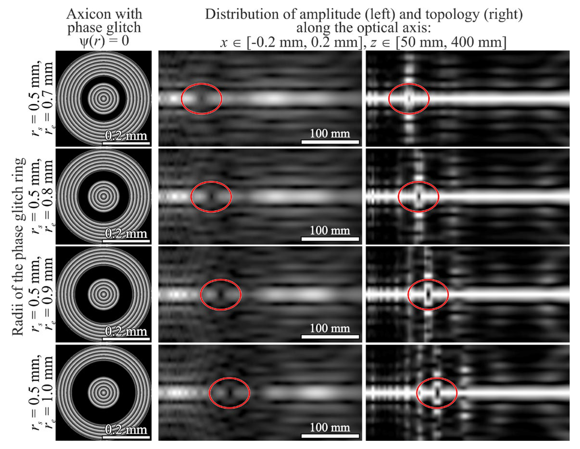
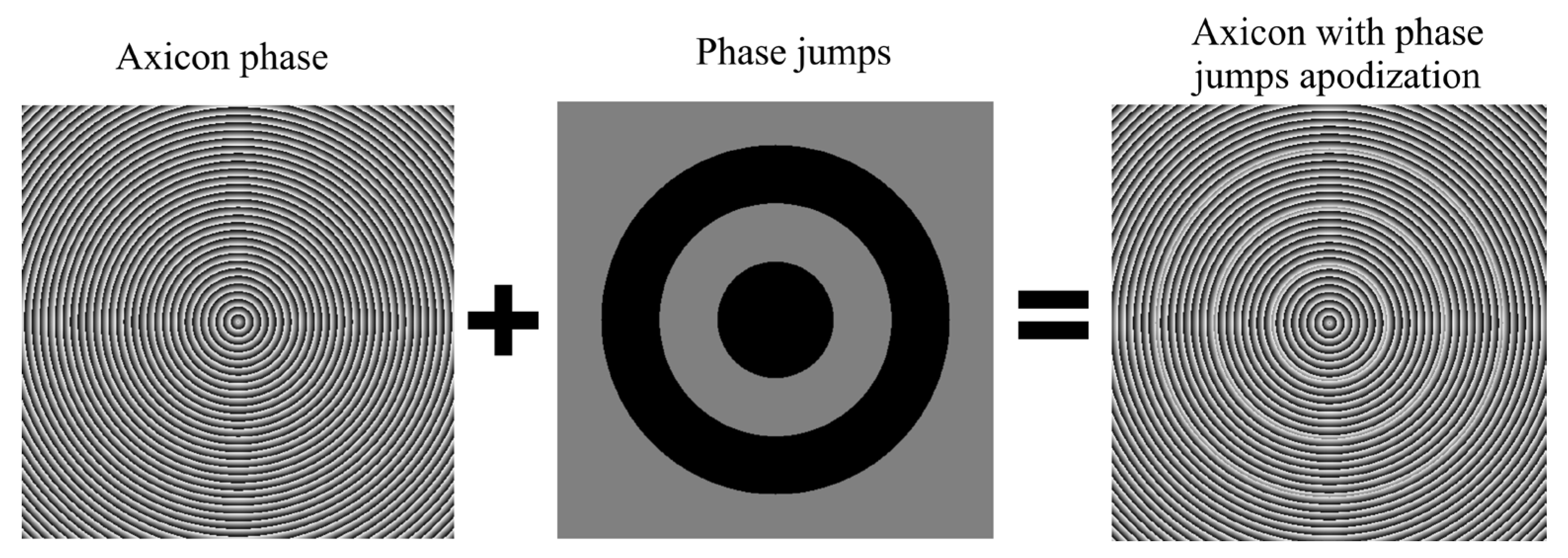
2.2.2. Formation of a Set of Optical Bottles Due to Phase Jumps on the Axicon

It should be noted that the approaches discussed in Section 2.1.2 and Section 2.2.1 are not very convenient for the formation of many optical bottles since, in this case, a large optical element is required.
To ensure the formation of a set of compactly located optical bottles, it is more convenient to use additional phase jumps in the axicon, which ensures the arrival of rays at a certain point on the optical axis with the opposite phase.
In this case, the optical element can be considered as an axicon with superimposed annular phase jumps (Figure 8):
τ p a x ( r ) = exp i k α r q = 1 Q exp i q π N q ( r )
where
N q ( r ) = 1 , r q s r r q e , 0 , else .
is the q-th ring with inner and outer radii rqs and rqe.
The element defined by Equation (22) provides zero intensity on the optical axis at points zq = rqs/α due to the arrival of rays in the antiphase. Figure 9 shows the results of modeling the formation of three optical bottles on the optical axis.
Note, in this case, the positions of the formed shadow regions corresponding to the optical bottles are very close to the geometric-optical positions. This type of apodization seems to us the most convenient and efficient for the formation of a set of optical bottles with a controlled position. A composite phase element calculated as illustrated in Figure 8 can be implemented using SLM.

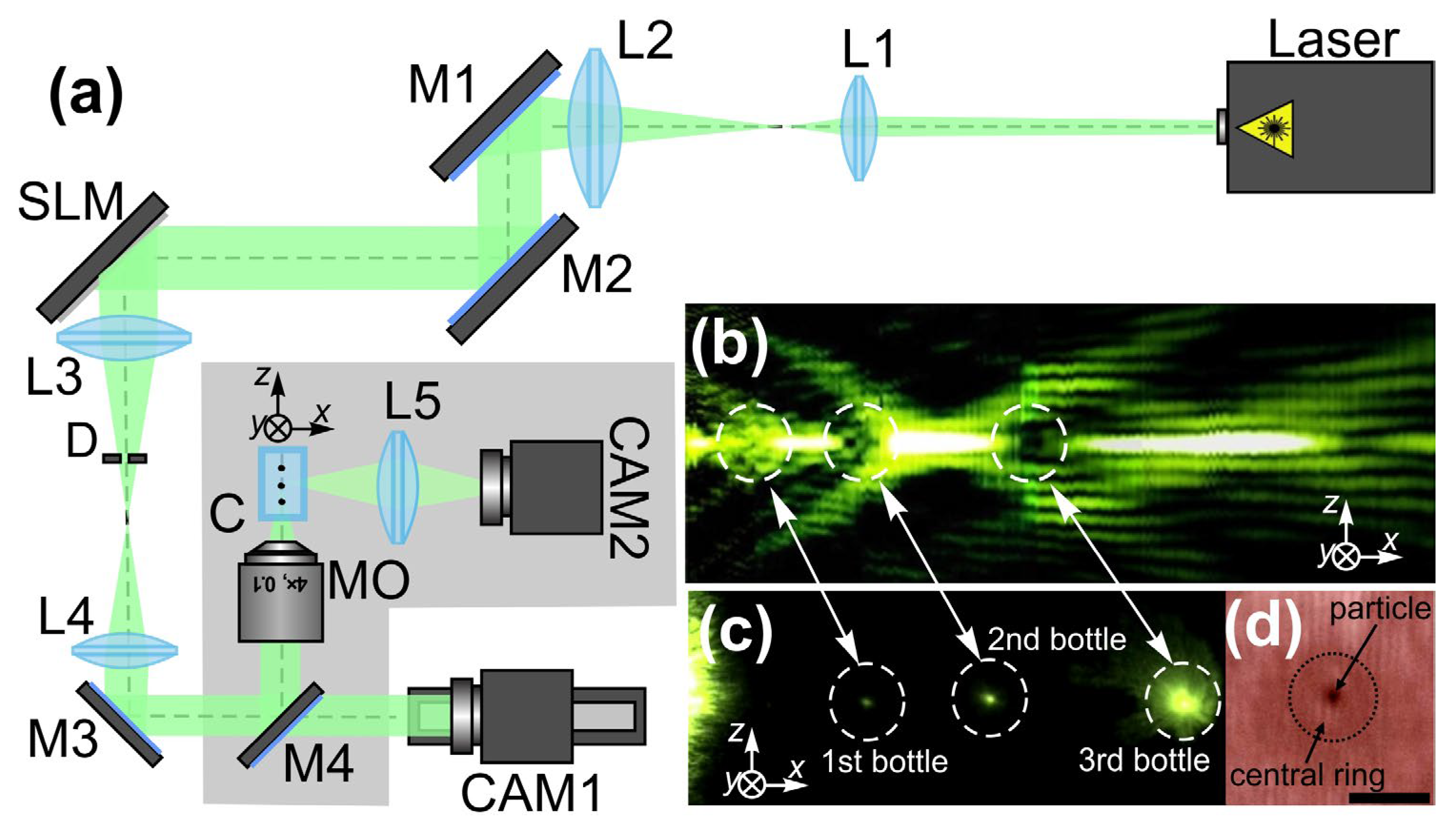
3. Experimental Results

For the experimental verification of the possibility of the generation of multiple optical bottle beams using the designed axicon with phase jumps, we used an optical setup based on a reflective SLM HOLOEYE PLUTO VIS (1920 × 1080 pixels, pixel size of 8 μm), which is shown in Figure 10a. A linearly polarized Gaussian beam from a solid-state continuous-wave laser (λ = 532 nm) was extended and collimated with a combination of two lenses, L1 and L2, with focal lengths of 25 and 150 mm. The maximum output laser power was 500 mW. The collimated laser beam was directed onto the SLM with the help of mirrors M1 and M2, and the modulated reflected laser beam was spatially filtered with a combination of two lenses, L3 and L4, with focal lengths of 500 and 150 mm, as well as a circular diaphragm D. In the experiments, we added a gradient phase mask to the phase of the designed element realized with the SLM to separate the generated multiple optical bottle beams and the part of the incident laser radiation that was not modulated by the SLM. Diaphragm D was used to block this non-modulated radiation. The diameter of the diaphragm was large enough not to eliminate the side robe of the generated Bessel beams. For reconstruction of the longitudinal intensity distribution of the generated multiple optical bottles shown in Figure 10b, a micro objective MO1 (4×, NA = 0.1) and a video camera CAM1 (TOUPCAM UHCCD00800KPA, 1600 × 1200 pixels, 3.34 μm pixel size) mounted on an optical rail were used. It is seen that the experimentally obtained intensity distributions are in good agreement with the numerically obtained ones.
The generated multiple optical bottle beams can be used as optical traps with increasing trapping stiffness for the light-absorbing particles in the air. It is well known that for such particles, the photophoretic (PP) forces dominate over the other forces [17,38]. However, in many cases, the direction of these forces is from the higher-intensity regions to the lower-intensity regions, which makes it impossible to realize stable three-dimensional trapping of light-absorbing particles using focused Gaussian beams. In these cases, optical bottle beams allow one to confine the trapped particles inside the dark intensity region and guide them stably in three dimensions. In our experiments, we used generated multiple optical bottles for trapping and stable confinement of light-absorbing agglomerations of carbon nanoparticles (the average density of approx. 10 mg/cm3, the thermal conductivity of 0.0266 W/m/K; an asymmetry factor of −0.34 [67]). The results obtained are shown in Figure 10c,d, and in Video S1 and Video S2. For these experiments, we slightly changed the optical setup used for the reconstruction of the longitudinal intensity distribution of the generated multiple optical bottles the changed part as shown in the grey area of Figure 10a. The micro objective MO2 (4×, NA = 0.1) was used to focus the modulated laser beam inside a glass cuvette C. Thus, generated multiple optical bottle beams were formed inside the cuvette. To load the particles into the generated traps, we sprayed carbon nanoparticles using a syringe. Then, a lens L5 and a video camera CAM2 were used to record a movie demonstrating trapping and confinement of the particles inside the generated traps (see Figure 10c). During the recording of the movie, the initial laser power decreased from 500 to 20 mW (Video S1). At the beginning of the recording, many particles were trapped in the generated laser beam. However, a decrease in the laser power led to the escape of unstable trapped particles from the beam. At a laser power of 20 mW, only three particles trapped in the three generated optical bottle beams remain trapped three-dimensionally stably (Video S2).

4. Conclusions

In this work, we investigated the generation of both light needles on the optical axis with a controllable location and optical bottle beams using an axicon with an amplitude or phase jump. The parameters of generated light needles, such as their length and their position on the axis, are defined by the axicon parameter α and the dimensions of the used annular aperture. We showed that the use of several annular apertures makes it possible to form a chain of light needles with a certain length and position. It was proposed to use this approach to form optical bottle beams at the desired location on the optical axis. In this case, the formation of an optical bottle occurs because of the blocking of the part of the illuminating laser beam by an annular screen. The light rays from the central and peripheral parts of the axicon form the “neck” and “bottom” of the bottle, and the cavity of the bottle is formed on the segment of the optical axis corresponding to the blocking ring. We showed that similar but more accurate and efficient results could also be obtained when we use an axicon with phase jumps. The numerically obtained results were approved by experiments. In addition, we showed laser trapping of three light-absorbing agglomerations of carbon nanoparticles in the air using the light fields generated by the designed axicons. Such optical traps find a lot of applications in optical manipulation and can be used for simultaneous trapping and guiding of several investigated particles that speed up the manipulation process.

Supplementary Materials

The following supporting information can be downloaded at: https://www.mdpi.com/article/10.3390/photonics10020200/s1. Video S1: three agglomerations of carbon nanoparticles trapped using the generated multiple op-tical bottles (xz-plane); Video S2: particle trapped in the first optical bottle observed in the transverse (xy) plane.

Author Contributions

Conceptualization: S.N.K. and S.I.K.; Methodology: S.N.K. and S.I.K.; Formal analysis: S.N.K. and A.V.U.; Software: S.N.K.; Investigation: S.N.K., S.A.F. and A.P.P.; Writing—original draft: S.N.K. and A.P.P.; Writing—Review and editing: S.N.K. and A.P.P.; Data curation: A.V.U.; Experimental realization: S.A.F. and A.P.P.; Visualization, A.P.P. and S.N.K.; Supervision, S.N.K.; Project administration, S.N.K.; Funding acquisition, A.P.P. All authors have read and agreed to the published version of the manuscript.

Funding

The work was supported by the Russian Science Foundation grant No. 22-12-00041 in the theoretical and experimental parts and by the Ministry of Science and Higher Education of the Russian Federation as part of the work under the State task of the Federal Research Center “Crystallography and Photonics” of the Russian Academy of Sciences (agreement No. 007-GZ/Ch3363/26) in parts of numerical simulation.

Institutional Review Board Statement

Not applicable.

Informed Consent Statement

Not applicable.

Data Availability Statement

Data will be made available on request.

Acknowledgments

We acknowledge the equal contribution of all the authors.

Conflicts of Interest

The authors declare that they have no known competing financial interests or personal relationships that could have appeared to influence the work reported in this paper.

References

  1. Ashkin, A.; Dziedzic, J.M.; Bjorkholm, J.E.; Chu, S. Observation of a Single-Beam Gradient Force Optical Trap for Dielectric Particles. Opt. Lett. 1986, 11, 288–290. [Google Scholar] [CrossRef] [PubMed]
  2. Ashkin, A.; Dziedzic, J.M.; Yamane, T. Optical Trapping and Manipulation of Single Cells Using Infrared Laser Beams. Nature 1987, 330, 769–771. [Google Scholar] [CrossRef] [PubMed]
  3. LaFratta, C.N. Optical Tweezers for Medical Diagnostics. Anal. Bioanal. Chem. 2013, 405, 5671–5677. [Google Scholar] [CrossRef] [PubMed]
  4. Hu, S.; Liao, Z.W.; Cai, L.; Jiang, X.X. Near-Field Optical Tweezers for Chemistry and Biology. Phys. Status Solidi A 2020, 217, 1900604. [Google Scholar] [CrossRef]
  5. Metcalf, H.J.; van der Straten, P. Laser Cooling and Trapping; Springer: New York, NY, USA, 1999; pp. 149–164. [Google Scholar]
  6. Bustamante, C.J.; Chemla, Y.R.; Liu, S.; Wang, M.D. Optical Tweezers in Single-Molecule Biophysics. Nat. Rev. Methods Prim. 2021, 1, 25. [Google Scholar] [CrossRef]
  7. Wang, M.D.; Yin, H.; Landick, R.; Gellse, J.; Block, S.M. Stretching DNA with Optical Tweezers. Biophys. J. 1997, 72, 1335–1346. [Google Scholar] [CrossRef]
  8. Zhong, M.-C.; Wei, X.-B.; Zhou, J.-H.; Wang, Z.-Q.; Li, Y.-M. Trapping Red Blood Cells in Living Animals Using Optical Tweezers. Nat. Commun. 2013, 4, 1768. [Google Scholar] [CrossRef]
  9. Chu, S.; Bjorkholm, J.E.; Ashkin, A.; Cable, A. Experimental Observation of Optically Trapped Atoms. Phys. Rev. Lett. 1986, 57, 314–317. [Google Scholar] [CrossRef]
  10. Dufresne, E.R.; Grier, D.G. Optical Tweezer Arrays and Optical Substrates Created with Diffractive Optical Elements. Rev. Sci. Instrum. 1998, 69, 1974–1977. [Google Scholar] [CrossRef]
  11. Curtis, J.E.; Koss, B.A.; Grier, D.G. Dynamic Holographic Optical Tweezers. Opt. Commun. 2002, 207, 169–175. [Google Scholar] [CrossRef]
  12. Forbes, A. Structured Light. Nat. Photon. 2021, 15, 253–262. [Google Scholar] [CrossRef]
  13. Arlt, J. Generation of a beam with a dark focus surrounded by regions of higher intensity: The optical bottle beam. Opt. Lett. 2000, 25, 191–193. [Google Scholar] [CrossRef]
  14. Yelin, D.; Bouma, B.E.; Tearney, G.J. Generating an adjustable three-dimensional dark focus. Opt. Lett. 2004, 29, 661–663. [Google Scholar] [CrossRef]
  15. Xiao, Y.; Yu, Z.; Wambold, R.A.; Mei, H.; Hickman, G.; Goldsmith, R.H.; Saffman, M.; Kats, M.A. Efficient generation of optical bottle beams. Nanophotonics 2021, 10, 2893–2901. [Google Scholar] [CrossRef]
  16. Shvedov, V.G.; Hnatovsky, C.; Rode, A.V.; Krolikowski, W. Robust trapping and manipulation of airborne particles with a bottle beam. Opt. Express 2011, 19, 17350–17356. [Google Scholar] [CrossRef]
  17. Alpmann, C.; Esseling, M.; Rose, P.; Denz, C. Holographic optical bottle beams. Appl. Phys. Lett. 2012, 100, 111101. [Google Scholar] [CrossRef]
  18. Gong, Z.; Pan, Y.-L.; Videen, G.; Wang, C. Optical trapping and manipulation of single particles in air: Principles, technical details, and applications. J. Quant. Spectrosc. Radiat. Transf. 2018, 214, 94–119. [Google Scholar] [CrossRef]
  19. Chaloupka, J.L.; Fisher, Y.; Kessler, T.J.; Meyerhofer, D.D. Single-beam, ponderomotive-optical trap for free electrons and neutral atoms. Opt. Lett. 1997, 22, 1021–1023. [Google Scholar] [CrossRef]
  20. Porfirev, A.P.; Skidanov, R.V. Generation of an array of optical bottle beams using a superposition of Bessel beams. Appl. Opt. 2013, 52, 6230–6238. [Google Scholar] [CrossRef]
  21. Cai, Y.; Lu, X.; Lin, Q. Hollow Gaussian Beams and Their Propagation Properties. Opt. Lett. 2003, 28, 1084–1086. [Google Scholar] [CrossRef]
  22. Wei, C.; Lu, X.; Wu, G.; Wang, F.; Cai, Y. A New Method for Generating a Hollow Gaussian Beam. Appl. Phys. B 2014, 115, 55–60. [Google Scholar] [CrossRef]
  23. Liu, Z.; Zhao, H.; Liu, J.; Lin, J.; Ahmad, M.A.; Liu, S. Generation of Hollow Gaussian Beams by Spatial Filtering. Opt. Lett. 2007, 32, 2076–2078. [Google Scholar] [CrossRef] [PubMed]
  24. Lu, L.; Wang, Z. Hollow Gaussian Beam: Generation, Transformation and Application in Optical Limiting. Opt. Commun. 2020, 471, 125809. [Google Scholar] [CrossRef]
  25. Ozeri, R.; Khaykovich, L.; Davidson, N. Long spin relaxation times in a single-beam blue-detuned optical trap. Phys. Rev. A 1999, 59, R1750–R1753. [Google Scholar] [CrossRef]
  26. Xia, M.; Wang, Z.; Yin, Y.; Zhou, Q.; Xia, Y.; Yin, J. Generation and Propagation Characteristics of a Localized Hollow Beam. Laser Phys. 2018, 28, 55001. [Google Scholar] [CrossRef]
  27. Philip, G.M.; Viswanathan, N.K. Generation of Tunable Chain of Three-Dimensional Optical Bottle Beams via Focused Multi-Ring Hollow Gaussian Beam. J. Opt. Soc. Am. A 2010, 27, 2394–2401. [Google Scholar] [CrossRef]
  28. Chremmos, I.; Zhang, P.; Prakash, J.; Efremidis, N.K.; Christodoulides, D.N.; Chen, Z. Fourier-space generation of abruptly autofocusing beams and optical bottle beams. Opt. Lett. 2011, 36, 3675–3677. [Google Scholar] [CrossRef]
  29. Chremmos, I.D.; Chen, Z.; Christodoulides, D.N.; Efremidis, N.K. Abruptly autofocusing and autodefocusing optical beams with arbitrary caustics. Phys. Rev. A 2012, 85, 23828. [Google Scholar] [CrossRef]
  30. Qian, Y.; Lai, S.; Mao, H. Generation of high-power bottle beams and autofocusing beams. IEEE Photon. J. 2018, 10, 6500607. [Google Scholar] [CrossRef]
  31. Ye, H.; Wan, C.; Huang, K.; Han, T.; Teng, J.; Ping, Y.S.; Qiu, C.W. Creation of Vectorial Bottle-Hollow Beam Using Radially or Azimuthally Polarized Light. Opt. Lett. 2014, 39, 630–633. [Google Scholar] [CrossRef]
  32. Shvedov, V.G.; Hnatovsky, C.; Shostka, N.; Krolikowski, W. Generation of Vector Bottle Beams with a Uniaxial Crystal. J. Opt. Soc. Am. B 2013, 30, 1–6. [Google Scholar] [CrossRef]
  33. Gerchberg, R.W.; Saxton, W.O. A practical algorithm for the determination of phase from image and diffraction plane pictures. Optik 1972, 35, 237–246. [Google Scholar]
  34. Kotlyar, V.V.; Khonina, S.N.; Soifer, V.A. Iterative calculation of diffractive optical elements focusing into a three dimensional domain and the surface of the body of rotation. J. Mod. Opt. 1996, 43, 1509–1524. [Google Scholar] [CrossRef]
  35. Zhang, J.; Pegard, N.; Zhong, J.; Adesnik, H.; Waller, L. 3D computer-generated holography by non-convex optimization. Optica 2017, 4, 1306–1313. [Google Scholar] [CrossRef]
  36. Kachalov, D.G.; Gamazkov, K.A.; Pavelyev, V.S.; Khonina, S.N. Optimization of binary DOE for formation of the “Light Bottle”. Comput. Opt. 2011, 35, 70–76. [Google Scholar]
  37. Pavelyev, V.; Osipov, V.; Kachalov, D.; Khonina, S.; Cheng, W.; Gaidukeviciute, A.; Chichkov, B. Diffractive optical elements for the formation of “light bottle” intensity distributions. Appl. Opt. 2012, 51, 4215–4218. [Google Scholar] [CrossRef]
  38. Turpin, A.; Shvedov, V.; Hnatovsky, C.; Loiko, Y.V.; Mompart, J.; Krolikowski, W. Optical vault: A reconfigurable bottle beam based on conical refraction of light. Opt. Express 2013, 21, 26335–26340. [Google Scholar] [CrossRef]
  39. Zhang, P.; Zhang, Z.; Prakash, J.; Huang, S.; Hernandez, D.; Salazar, M.; Christodoulides, D.N.; Chen, Z. Trapping and transporting aerosols with a single optical bottle beam generated by moiré techniques. Opt. Lett. 2011, 36, 1491–1493. [Google Scholar] [CrossRef]
  40. de Angelis, M.; Cacciapuoti, L.; Pierattini, G.; Tino, G.M. Axially symmetric hollow beams using refractive conical lenses. Opt. Lasers Eng. 2003, 39, 283–291. [Google Scholar] [CrossRef]
  41. Wei, M.-D.; Shiao, W.-L.; Lin, Y.-T. Adjustable generation of bottle and hollow beams using an axicon. Opt. Commun. 2005, 248, 7–14. [Google Scholar] [CrossRef]
  42. Lin, J.H.; Wei, M.D.; Liang, H.H.; Lin, K.H.; Hsieh, W.F. Generation of supercontinuum bottle beam using an axicon. Opt. Express 2007, 15, 2940–2946. [Google Scholar] [CrossRef] [PubMed]
  43. Zeng, X.; Wu, F. The analytical description and experiments of the optical bottle generated by an axicon and a lens. J. Mod. Opt. 2008, 55, 3071–3081. [Google Scholar] [CrossRef]
  44. Khonina, S.N.; Porfirev, A.P. 3D transformations of light fields in the focal region implemented by diffractive axicons. Appl. Phys. B 2018, 124, 191. [Google Scholar] [CrossRef]
  45. Khonina, S.N.; Porfirev, A.P.; Volotovskiy, S.G.; Ustinov, A.V.; Fomchenkov, S.A.; Pavelyev, V.S.; Schröter, S.; Duparré, M. Generation of multiple vector optical bottle beams. Photonics 2021, 8, 218. [Google Scholar] [CrossRef]
  46. Daria, V.R.; Rodrigo, P.J.; Glückstad, J. Dynamic array of dark optical traps. Appl. Phys. Lett. 2004, 84, 323–325. [Google Scholar] [CrossRef]
  47. Mcleod, J.H. The Axicon: A New Type of Optical Element. J. Opt. Soc. Am. 1954, 44, 592–597. [Google Scholar] [CrossRef]
  48. Khonina, S.N.; Kazanskiy, N.L.; Khorin, P.A.; Butt, M.A. Modern Types of Axicons: New Functions and Applications. Sensors 2021, 21, 6690. [Google Scholar] [CrossRef]
  49. Akturk, S.; Arnold, C.L.; Prade, B.; Mysyrowicz, A. Generation of high quality tunable Bessel beams using a liquid-immersion axicon. Opt. Commun. 2009, 282, 3206–3209. [Google Scholar] [CrossRef]
  50. Khonina, S.N.; Kazanskiy, N.L.; Karpeev, S.V.; Butt, M.A. Bessel Beam: Significance and Applications—A Progressive Review. Micromachines 2020, 11, 997. [Google Scholar] [CrossRef]
  51. Garces-Chavez, V.; McGloin, D.; Melville, H.; Sibbett, W.; Dholakia, K. Simultaneous micromanipulation in multiple planes using a self-resonstructing light beam. Nature 2002, 419, 145–147. [Google Scholar] [CrossRef]
  52. Gori, F.; Guattari, G.; Padovani, C. Bessel-Gauss beams. Opt. Commun. 1987, 64, 491–495. [Google Scholar] [CrossRef]
  53. Krasin, G.K.; Vinogradov, M.A.; Kovalev, M.S.; Nosov, P.A. Investigation of parameters of the Bessel beam formed by an axicon. Proc. SPIE 2019, 11028, 110281Q. [Google Scholar] [CrossRef]
  54. Stsepuro, N.; Nosov, P.; Galkin, M.; Krasin, G.; Kovalev, M.; Kudryashov, S. Generating Bessel-Gaussian Beams with Controlled Axial Intensity Distribution. Appl. Sci. 2020, 10, 7911. [Google Scholar] [CrossRef]
  55. Gorelick, S.; Paganin, D.M.; Korneev, D.; De Marco, A. Hybrid refractive-diffractive axicons for Bessel-beam multiplexing and resolution improvement. Opt. Express 2020, 28, 12174–12188. [Google Scholar] [CrossRef]
  56. Monsoriu, J.A.; Furlan, W.D.; Andrés, P.; Lancis, J. Fractal conical lenses. Opt. Express 2006, 14, 9077–9082. [Google Scholar] [CrossRef]
  57. Mihailescu, M.; Preda, A.M.; Sobetkii, A.; Petcu, A.C. Fractal-like diffractive arrangement with multiple focal points. Opto-Electron. Rev. 2009, 17, 330–337. [Google Scholar] [CrossRef]
  58. Zhu, L.; Yu, J.; Zhang, D.; Sun, M.; Chen, J. Multifocal spot array generated by fractional Talbot effect phase-only modulation. Opt. Express 2014, 22, 9798–9808. [Google Scholar] [CrossRef]
  59. Khonina, S.N.; Volotovsky, S.G. Fractal cylindrical fracxicon. Opt. Mem. Neural Netw. 2018, 27, 1–9. [Google Scholar] [CrossRef]
  60. Rastani, K.; Marrakchi, A.; Habiby, S.F.; Hubbard, W.M.; Gilchrist, H.; Nahory, R.E. Binary phase Fresnel lenses for generation of two-dimensional beam arrays. Appl. Opt. 1991, 30, 1347–1354. [Google Scholar] [CrossRef]
  61. Khonina, S.N.; Ustinov, A.V.; Skidanov, R.V.; Porfirev, A.P. Local foci of a parabolic binary diffraction lens. Appl. Opt. 2015, 54, 5680–5685. [Google Scholar] [CrossRef]
  62. Davis, J.A.; Moreno, I.; Martinez, J.L.; Hernandez, T.J.; Cottrell, D.M. Creating three-dimensional lattice patterns using programmable Dammann gratings. Appl. Opt. 2011, 50, 3653–3657. [Google Scholar] [CrossRef] [PubMed]
  63. Zhu, L.; Sun, M.; Zhu, M.; Chen, J.; Gao, X.; Ma, W.; Zhang, D. Three-dimensional shape-controllable focal spot array created by focusing vortex beams modulated by multi-value pure-phase grating. Opt. Express 2014, 22, 21354–21367. [Google Scholar] [CrossRef] [PubMed]
  64. Khonina, S.N.; Porfirev, A.P.; Ustinov, A.V. Sudden autofocusing of superlinear chirp beams. J. Opt. 2018, 20, 25605. [Google Scholar] [CrossRef]
  65. Friberg, A.T. Stationary-phase analysis of generalized axicons. J. Opt. Soc. Am. A 1996, 13, 743–750. [Google Scholar] [CrossRef]
  66. Ustinov, A.V.; Khonina, S.N. Generalized lens: Calculation of distribution on the optical axis. Comput. Opt. 2013, 37, 307–315. [Google Scholar] [CrossRef]
  67. Porfirev, A.P.; Dubman, A.B.; Porfiriev, D.P. Demonstration of a simple technique for controllable revolution of light-absorbing particles in air. Opt. Lett. 2020, 45, 1475–1478. [Google Scholar] [CrossRef]
Figure 1. (a) View of the annular slot. (b) Geometric-optical illustration of the formation of a light segment on the optical axis.
Photonics 10 00200 g001
Figure 2. Simulation results of the formation of axial light segments with different lengths and positions due to variations in the parameters of the annular aperture were obtained using Equation (2).
Photonics 10 00200 g002
Figure 3. Illustration of the formation of an optical bottle due to radiation blocking by an annular screen: (a) view of the annular slot and (b) geometric-optical visualization of the formation of an optical bottle on the optical axis.
Photonics 10 00200 g003
Figure 4. Simulation results of the optical bottle formation by blocking radiation using an annular screen under illumination with a flat beam: (a) amplitude and (b) phase at the input, (c) amplitude distribution along the optical axis (x∈[−0.5 mm; 0.5 mm], z∈[50 mm; 400 mm]), (d) plot of intensity on the axis for the annular slots rs = 0, re = 0.5 mm (blue color), rs = 0.7 mm, re = 1.5 mm (green color) and for the blocking screen rs = 0.5 mm, re = 0.7 mm (red color).
Photonics 10 00200 g004
Figure 5. Simulation results of the optical bottle formation by blocking radiation using an annular screen under illumination with the Gaussian beam with σ = 1.3 mm: (a) amplitude and (b) phase at the input, (c) amplitude distribution along the optical axis (x∈[−0.5 mm; 0.5 mm], z∈[50 mm; 400 mm]), (d) plot of intensity on the axis for the annular slots rs = 0, re = 0.5 mm (blue color), rs = 0.7 mm, re = 1.5 mm (green color) and for the blocking screen rs = 0.5 mm, re = 0.7 mm (red color).
Photonics 10 00200 g005
Figure 6. Comparative modeling of the optical bottles formation due to radiation blocking by an annular screen under illumination with a bounded flat and the Gaussian beam (the amplitude distribution along the optical axis is shown x∈[−0.2 mm; 0.2 mm], z∈[50 mm; 400 mm]).
Photonics 10 00200 g006
Figure 7. Modeling results for the formation of optical bottles due to axicons with phase apodization ψ(r) = 0 in Equation (21) under Gaussian beam illumination.
Photonics 10 00200 g007
Figure 8. Illustration of axicon apodization by phase jumps (π-shifts between black and grey).
Photonics 10 00200 g008
Figure 9. Simulation of the formation of three optical bottles due to phase jumps at radii r1s = 0.4 mm, r1e = r2s = 0.6 mm, r2e = r3s = 1.0 mm on the axicon under Gaussian beam illumination with σ = 1.3 mm: (a) amplitude and (b) phase at the input, (c) amplitude distribution along the optical axis (x∈[–0.2 mm; 0.2 mm], z∈[50 mm; 400 mm]), (d) intensity plot on the axis with the corresponding geometric positions of the optical traps z1 = 80 mm, z2 = 120 mm, z3 = 200 mm (marked by red lines).
Photonics 10 00200 g009
Figure 10. Optical trapping with multiple optical bottles generated an axicon with phase jumps. (a) The optical setup used for the generation of the desired multiple optical bottles: Laser is a solid-state laser (λ = 532 nm), L1, L2, L3, L4, and L5 are lenses with focal lengths of 25, 150, 500, 150, and 50 mm respectively, M1, M2, M3, and M4 are mirrors, SLM is a reflective spatial light modulator HOLOEYE PLUTO VIS (1920×1080 pixels, pixel size of 8 μm), D is a circular diaphragm, MO is a micro objective (4×, NA = 0.1), C is a glass cuvette, CAM1 and CAM are video cameras (TOUPCAM UHCCD00800KPA, 1600 × 1200 pixels, 3.34 μm pixel size). (b) The longitudinal intensity distribution of the generated multiple optical bottles. The white dashed circles show the dark regions of the generated traps. (c) An image of three agglomerations of carbon nanoparticles (indicated by the white dashed circles) trapped using the generated multiple optical bottles (Video S1). In the left part of the image, the light scattered by a wall of the glass cuvette is shown. (d) An image of the particle trapped in the first optical bottle observed in the transverse (xy) plane (Video S2). The scale bar is 20 µm.
Photonics 10 00200 g010
Disclaimer/Publisher’s Note: The statements, opinions and data contained in all publications are solely those of the individual author(s) and contributor(s) and not of MDPI and/or the editor(s). MDPI and/or the editor(s) disclaim responsibility for any injury to people or property resulting from any ideas, methods, instructions or products referred to in the content.

