Abstract
Deep neural networks (DNNs) have been employed in continuous-variable quantum key distribution (CV-QKD) systems as attacking detection portions of defense countermeasures. However, the vulnerability of DNNs leaves security loopholes for hacking attacks, for example, adversarial attacks. In this paper, we propose to implement the one-pixel attack in CV-QKD attack detection networks and accomplish the misclassification on a minimum perturbation. This approach is based on the differential evolution, which makes our attack algorithm fool multiple DNNs with the minimal inner information of target networks. The simulation and experimental results show that, in four different CV-QKD detection networks, , , , and of the input data can be perturbed to another class by modifying just one feature, the same as one pixel for an image. We carry out this success rate in the context of the original accuracy reaching up to nearly on average. Further, by enlarging the number of perturbed features, the success rate can be raised to a satisfactory higher level of about . According to our experimental results, most of the CV-QKD detection networks can be deceived by launching one-pixel attacks.
1. Introduction
Quantum key distribution (QKD) [1] enables two remote correspondents, usually called Alice and Bob, to exchange secret keys in an information-theoretically secure way. According to the basic law of quantum mechanics, primarily the Heisenberg’s uncertainty principle [2] and the quantum no-cloning theorem [3], if there is an eavesdropper called Eve, the illegal measurements of Eve can be recognized by the legal receiver Bob and remove the leakage information. Taking the different implementation methods as the basis for classification, QKD can be divided into two categories: discrete-variable quantum key distribution (DV-QKD) [4,5] and continuous-variable quantum key distribution (CV-QKD) [6,7,8,9]. Previous researches have show that CV-QKD not only has a higher key rate but it is also easier to prepare and measure compared with DV-QKD. Additionally, CV-QKD is compatible with the existing optical networks, which provides it with an attractive future in a practical application. Here in this paper, our study is based on the CV-QKD system under its most practical protocol, a Gaussian-modulated coherent state (GMCS) protocol [10,11], which has been proven to be secure under collective attacks and coherent attacks in theory [12,13].
However, when it comes to an application in reality, the real CV-QKD system faces several security loopholes caused by the imperfection of realistic devices. The eavesdroppers in reality can break the security of the practical GMCS CV-QKD with attack strategies such as wavelength attacks [14,15], calibration attacks [16], local oscillator (LO) intensity attacks [17], saturation attacks [18], and homodyne-detector-blinding attacks [19]. To defend these practical attack strategies, diversified methods have been proposed. One type of defense method attempts to establish a new QKD protocol, such as device-independent QKD [20] and measurement device-independent QKD [21]. However, these protocols have shown a low key rate in previous practical research. Another typical defense method is to add security patches in the existing protocol, which probably leads to new loopholes by patching [22]. The other kind of countermeasure is to detect the timely parameter by adding relevant real-time monitoring modules on the system.
In recent years, with the swift development of artificial intelligence (AI) [23], many innovations based on the artificial neural network (ANN) has been proven to be effective. For example [24], Mao et al. [25] proposed an ANN model to classify their attack strategy, Luo et al. [26] proposed a semi-supervised deep learning method to detect known attacks and potential unknown attacks, and Du et al. [27] proposed an ANN model for multi-attacks detection. The main idea of these methods is to implement specific defense countermeasures based on the classification result from the ANN model. However, the defense countermeasures which depend on the ANN can also bring new potential security threats to the CV-QKD system. According to the theory of an adversarial attack [28], particular tiny perturbations on the input vector are capable of misclassifying the original input, which can be an enormous threat to this security-sensitive system.
In this paper, we propose that a classical adversarial attack, the one-pixel attack [29], can be applied in the QKD field, directly against the CV-QKD defense countermeasures based on the DNNs classification. The schematic diagram of the CV-QKD systems that we attack is shown in Figure 1. In the experiment, we use a 1310 nm light source as our system independent clock. The pulse passes are split into the signal light source and the clock light source by a coarse wavelength-division multiplexing (CWDM) after reaching Bob. Then we take the separated 1310 nm light source as the system clock, which is used to monitor the real-time shot noise variance. The rest part of the pulses will pass a polarization beam splitter (PBS) after the CWDM to divide the signal pulses and the LO pulses. Next, the LO pulses are separated by a beam splitter (BS) to monitor the LO intensity and are sent to the next BS, respectively. The second BS will split the pulses into two parts for shot noise monitoring and homodyne detection with the signal being processed by an amplitude modulator. At last, those measurement results will come to the data preprocessing portion and be conducted as the original data which can be used in a neural network model for attack detection.
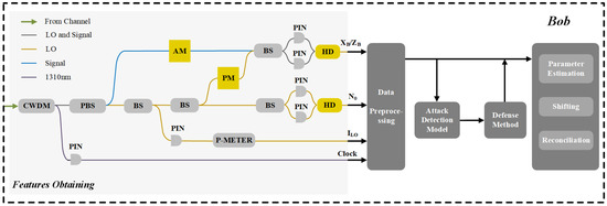
Figure 1.
Schematic diagram of applying one-pixel attack in a CV-QKD system to deceive the attack detection portion. CWDM: coarse wavelength-division multiplexing. PBS: polarization beam splitter. AM: amplitude modulator. PM: phase modulator. PIN: PIN photodiode. HD: homodyne detector. P-METER: the power meter to monitor LO intensity. Clock: clock circuit used to generate clock signal for measurement.
Considering the universality of the attacked models, we establish four representative DNNs, which are trained to distinguish the categories of attacks from three known attacks, one hybrid strategy attack, and the normal state as our attack targets. We migrate the method of the one-pixel attack, which is mostly based on a differential evolution (DE) algorithm [30], into these CV-QKD attack-detecting networks and investigate the prediction results of the perturbed data. Our experimental results have demonstrated that the one-pixel attack can be successfully removed from the image identification field to the CV-QKD attacking detection field. In addition, by slightly enlarging the number of perturbed pixels, we can significantly enhance the success rate of our attack. At last, we discuss the merit and demerit of our attacking strategy.
The paper is organized as follows. First, in Section 2, we introduce the dataset and methods used in our work, including the DNNs subjected to adversarial attacks and the algorithm details of the one-pixel attack. Then, we analyze the related simulation results of our attack strategy and discuss its merit and demerit in Section 3. Finally, we make a summary of our work in Section 4.
2. Materials and Methods
2.1. Datasets and Parameter Settings
In a CV-QKD system based on the GMCS protocol, Alice generates two continuous variable sets, x and p, which obey the Gaussian distribution with a zero average and variance . Then, by modulating weak coherent states , Alice encodes the key information and sends the encoded information to Bob through a strong of intensity . On the receiving end, with the phase reference extracted from , Bob can measure one of the quadratures of the signal states by performing a homodyne detection. After repeating this procedure various times, Bob will receive the correlated data sequence . The mean and variance of a receiving sequence can be described by:
where T and are the quantum channel transmittance and the efficiency of the homodyne detector, respectively. is the detector’s electronic noise and is the technical excess noise of the system.
To match with the existing classification networks of the CV-QKD attacks, our data consists of a normal condition, three kinds of common CV-QKD attacks: calibration attacks, local oscillator () intensity attacks, and saturation attacks, and one hybrid attack strategy consisting of intensity attacks and wavelength attacks. From another perspective, the classification network designed to distinguish the above-mentioned attack strategies is the most practical, since the individual wavelength attacks are only practicable in heterodyne detection CV-QKD systems. Here we obtain the labels of our dataset: .
According to Luo et al. and Mao et al. [25,26], there are some features that can be measured without disturbing the normal transmission between Alice and Bob. Among them, we select the intensity of the , the shot noise variance , the mean value , and the variance of Bob’s measurement as the features we use to distinguish diverse attack strategies. The value of these four features will change in a different degree after the CV-QKD process is attacked by different strategies. Therefore, we construct the vector to describe the security status of the communication as our feature vector.
The steps of preparing our dataset contain four following parts. First of all, for each of the CV-QKD attack strategies, including the normal condition, we generate the original sampling dataset of pulses in chronological order. Second, to acquire the statistical characteristics from the sampling characteristics, all pulses in the original data are divided into M time boxes including sets of sampling data in each box. Then we calculate the four statistical characteristics of each time box to obtain the feature vector . At last, in order to accommodate the universal ANN models in the image field and strengthen the stability of the input data as well, we combine 25 continuous feature vectors as an input matrix, which can be seen as a 25 × 4 image with one channel. The choice of this number refers the experiments of Luo et al. [26] and Du et al. [27]. The group generated here is the basic unit for our network to classify. At this point, we have five original datasets of each CV-QKD attack strategy. To build the rational training set and test set, 750 groups are randomly selected from each original dataset and divided into the training set and test set by a ratio of 2:1. Then we put all groups for training together to make a disrupted order and repeat this process to generate the test set. So far, the dataset for the model training and adversarial attack is well prepared. The rest of the details regarding the parameter setting and data perpetration are shown in Appendix A.
2.2. Models Architecture and Training Results
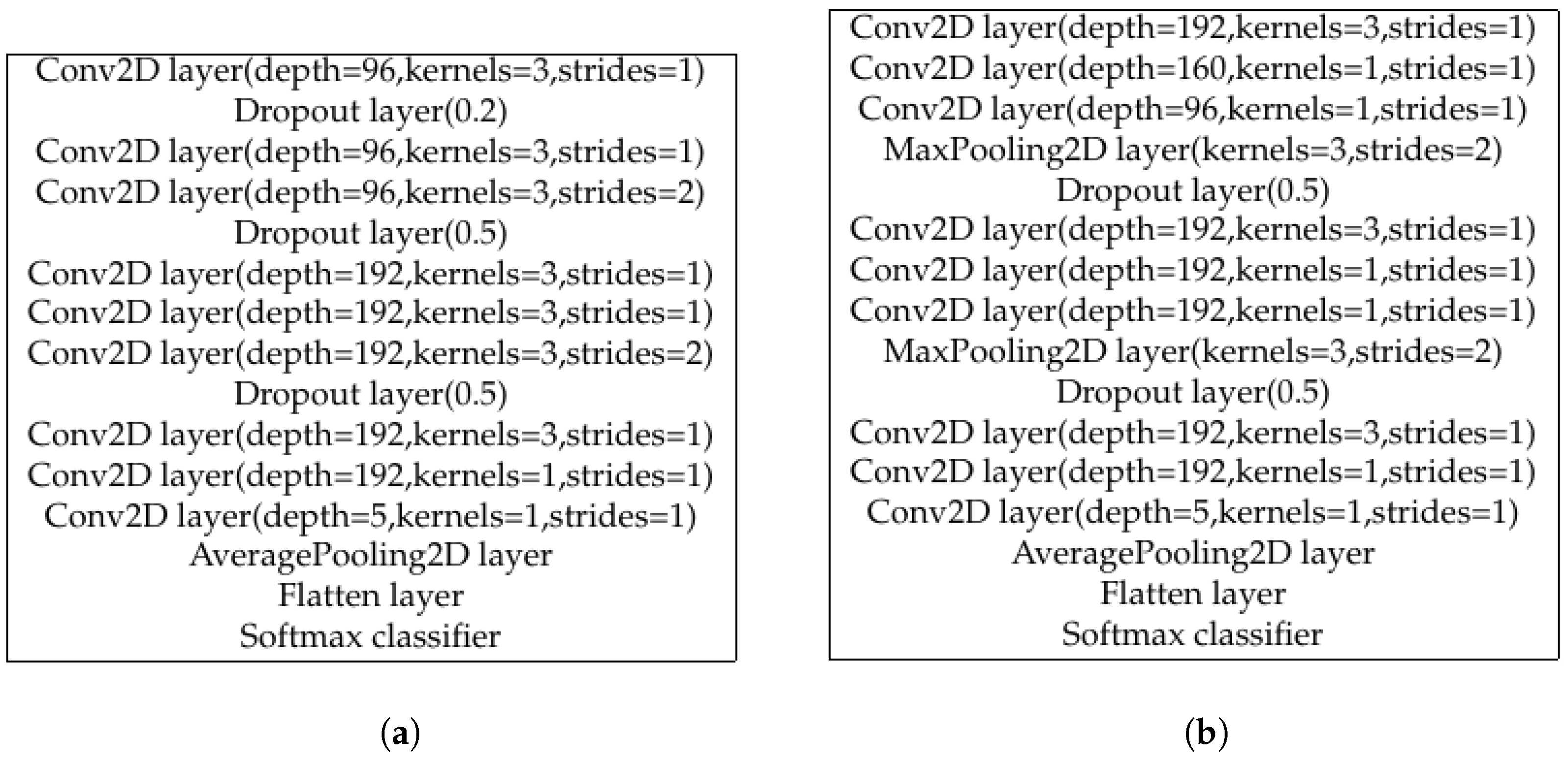
The significance of the CV-QKD attack detection models in our work can be mainly described in following two points. First of all, to conduct a one-pixel attack, we require numerous well-trained models as the scoring function. Second, the output labels of the models are the main metric to measure the effectiveness of our attack. According to the research of Jiawei Su et al. [29], which is the first to propose the one-pixel attack in the image field, this attack algorithm is effective in many deep neural networks, such as the all convolution network (AllConv), Network in Network (NiN) [31], Visual Geometry Group Network (VGG16) [32], and AlexNet. In our work, we select two classical models, AllConv and NiN, and additionally append two kinds of widely used DNNs, ResNet [33], and DenseNet [34] to validate our attack effect. The model training and attack simulation are programmed in Python with the help of its provided packages and some fundamental open source code; the dataset is generated in Matlab R2019b. The detailed structures of the AllConv and NiN network can be seen in Figure 2a,b, while the rest of the information is presented in Appendix B. Since the input matrix is relatively simpler than the initially designed input of the image information for the models, we predigest the structures slightly. Note that some dropout layers are added to our models compared with the original. We make these modifications in order to achieve a higher classification accuracy, which is proven to be effective by our tests. The standardized method is also used in data preprocessing in our work. In this way, the huge discrepancy between the measuring units of the different features can be mapped to a comparable range.

Figure 2.
The brief structures of an AllConv model and a NiN model for CV-QKD attack detection. (a) The structure of our AllConv network. (b) The structure of our NiN network. More detailed introduction can be seen in Appendix B. AllConv: all convolution network. NiN: Network in Network.
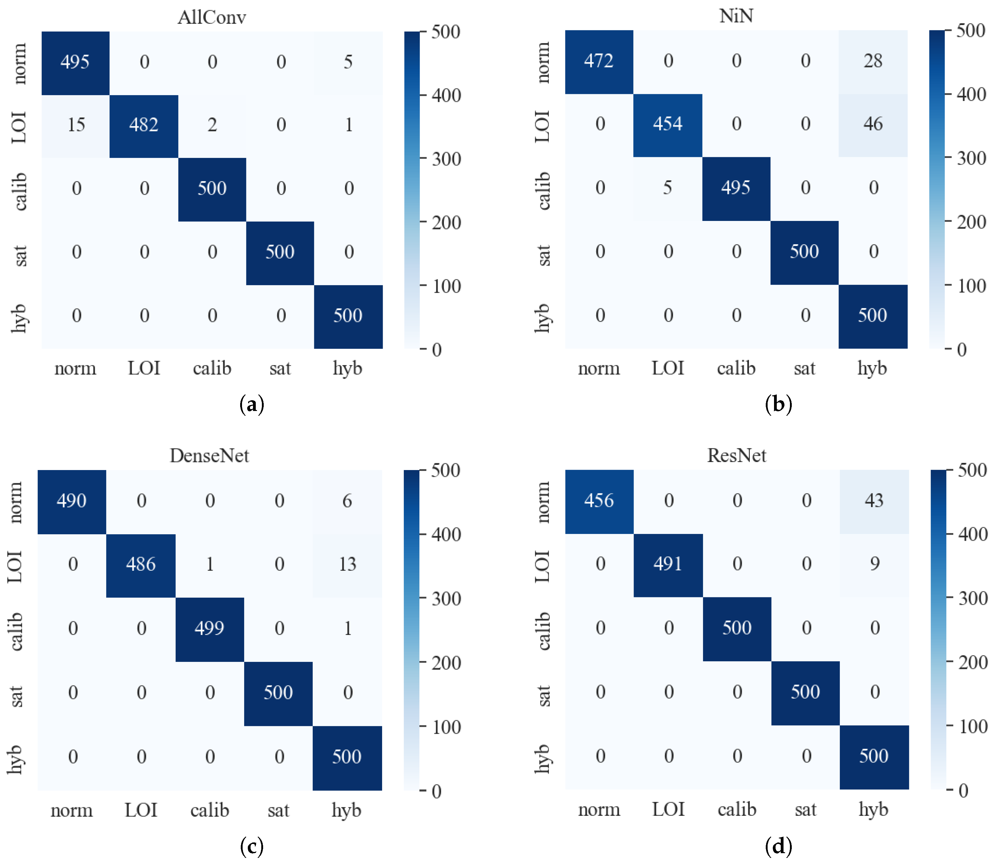
The performances of the trained models are shown in Table 1 and Figure 3. We select the most appropriate hyper-parameter value of epochs and batch size from and based on both the accuracy and efficiency. According to the consequence, the accuracy of the test set can reach a satisfactory result of on average. In Figure 3, most of the data fall on the diagonal of the confusion matrix, which visually shows the high accuracy of the four attack-detecting models.

Table 1.
The optimal hyper-parameter setting and predicting performance of the four networks for CV-QKD attack detection. Epochs refer to the turn number of iterate over the dataset. Batch Size refers to the number of data we used in one iteration. AllConv: all convolution network. NiN: Network in Network.
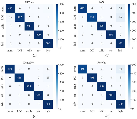
Figure 3.
The confusion matrices of the four networks for CV-QKD attack detection. (a) The predicting results of AllConv model. (b) The predicting results of NiN model. (c) The predicting results of DenseNet model. (d) The predicting results of ResNet model. AllConv: all convolution network. NiN: Network in Network. Norm: the unattacked state. LOI: LO intensity attacks. Calib: calibration attacks. Sat: saturation attacks. Hyb: the hybrids attacks.
2.3. Attacking Algorithm
As the research develops further, DNNs start to be applied to some safety-critical environments, for example, to the quantum communication. Therefore, the security of the DNNs draws the attention of numerous researchers. Amounts of previous studies suggest that DNNs are vulnerable to some specifically designed input samples which are similar to the original one; we call these adversarial examples. The one-pixel attack is a representative strategy to generate adversarial examples by only perturbing the input with a minimum of one pixel. Its approach can be described as the following formula:
where refers to the original input vector, refers to the perturbation, d is the number of perturbed pixels, and is the confidence of the target class.
The core advantages of the one-pixel attack can be concluded as three points below.
- First, it can execute an attack only relying on the probability labels of the target network without any inner information.
- Second, the attacking accuracy of the Kaggle CIFAR-10 dataset is regarded as high-efficiency. By only disturbing one pixel of a input image, it acquires a success rate above .
- Third, it can be flexibly used on most of the DNNs according to its basic theory, differential evolution (DE).
For a CV-QKD attacks detection network, the structure is generally designed as a DNN, which guarantees the feasibility of launching a one-pixel attack. Considering the compatibility, we rebuild the one-pixel attack on the basis of its original approach and DE algorithm. The frame of our attacking method is shown in Figure 4. The blue blocks in the frame are the four main parts of DE, which are used to find the most influential point to the classification result among an input matrix.

Figure 4.
The frame of the one-pixel attack in CV-QKD detection networks. The blue blocks represent the four core steps of DE algorithm: initial, mutation, crossover, and selection.
DE is a global optimization algorithm based on population-ecology theory. Generally, in each generation, primordial children will generate according to their parents. Then they will be used in a comparison with the parents, the results of which decide whether they can survive. The survivors will compose the new parents and give birth to the new generation to pass down their “genes”, what we call features in machine learning. By iteration, the last generation would be a convergent outcome, which is the most fraudulent perturbation we want to find.
To implement it specifically, the whole process can be divided into three main parts: the mutation, crossover, and selection. We assume the notation representing the ith individual in the population of with D dimension:
where , , .
First of all, the initial generation is created randomly by a certain distribution, usually a uniform distribution in the bounds in order to cover its range as much as we could. So, the first generation is initialized as:
where and describe the boundary of the output value.
Then the population starts to mutate depending on the following formula:
where p, r, and q are integers randomly chosen from the range and are different from each other at the same time. F is the mutation factor, which is settled as 0.5 usually.
A crossover step is carried out to enhance the diversity of the population. There are two ways to realize this goal:
where is called the crossover rate.
In the last step of one iteration, we select the individual between the parents and children depending on their performance in the score function. The selecting principle can be described as:
where represents the score function.
The steps mentioned above are the core method used in the one-pixel attack. According to this theory, we reset some parameters to adapt the dataset of the CV-QKD attack detection. Different from the RGB features of the images, the value of the input features is consecutive in their value domain. It means that there is infinite possible values for each feature, which forces us to augment the number of the population maximum . We have also attempted to enhance the attack by increasing the upper limit of the iterations. However, for the enormous amount of time consumed during the process, the slight change in the success rate is unworthy. As a result, we still use 100 as the limit superior to the iterations. In addition, the bounds of the different features are not unified. For the image input matrix, each RGB channel has the same boundary of [0, 255], whereas the four indicators of the CV-QKD attacks are in a different order of magnitude. To solve this problem, we add a normalization process as follows:
where is the output of DE and is a perturbed feature (one pixel) in the input matrix.
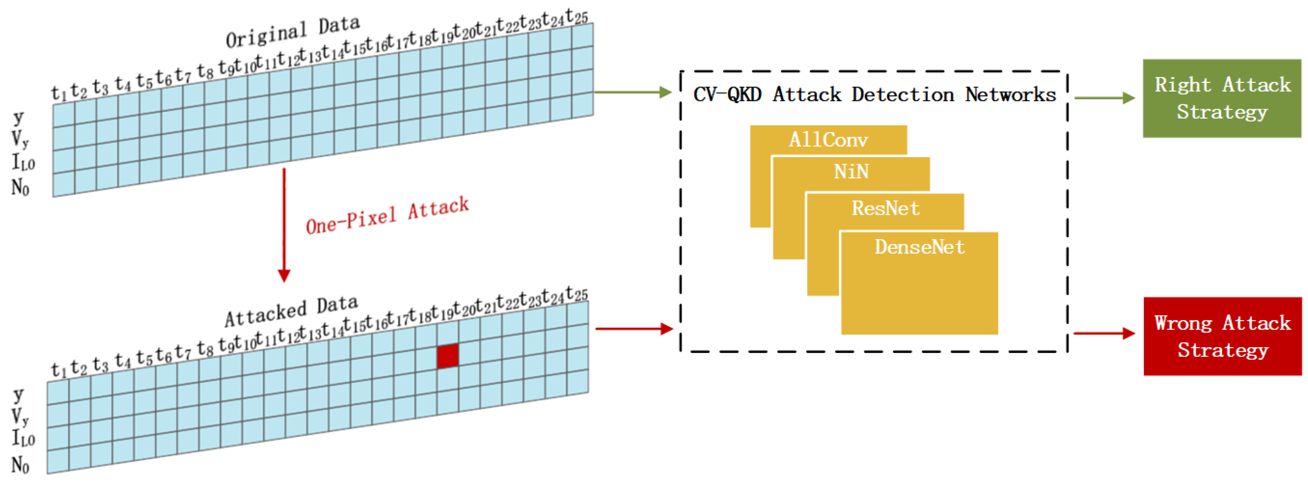
In this way, we generally finish the fundamental modification for the migration of the one-pixel attack into CV-QKD attacks detection. Using this method, an optimal perturbation for deceiving the CV-QKD attacks detection networks can be found, among each input matrix, shown in Figure 5. In the next section, we will display the performance of our work and draw a conclusion by analyzing the results.
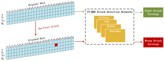
Figure 5.
The diagram of the attacking effect of one-pixel attacks for a CV-QKD system in our experiment. The detection networks are settled as AllConv, NiN, ResNet, and DenseNet. AllConv: all convolution network. NiN: Network in Network.
3. Results
3.1. Evaluation Indicators
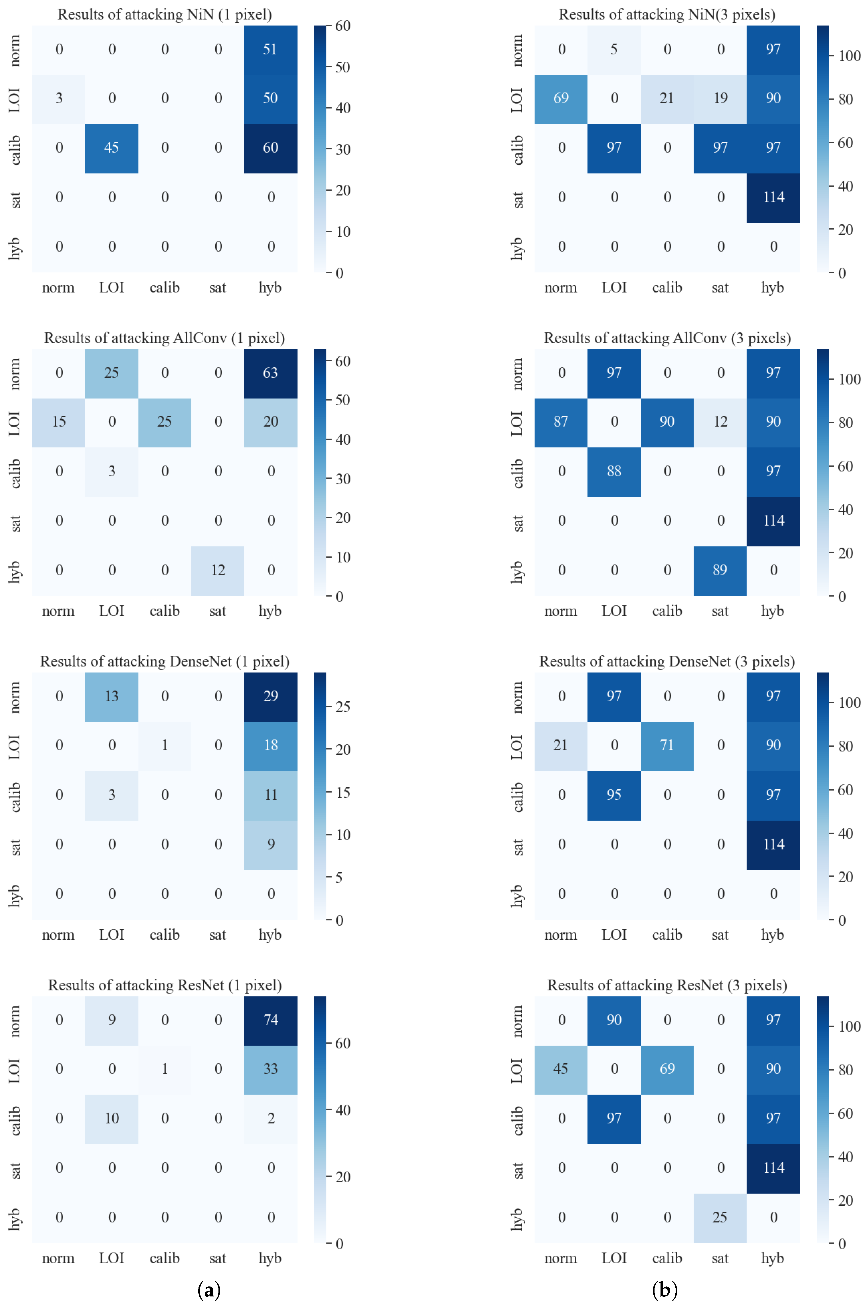
To verify the actual performance of our adversarial attack, we create a brand new set of data as the attacking objects. This objective dataset includes 500 groups of data randomly chosen from the test set, where the five attack strategies are almost mixed in the same proportion. Then, we carry out a four times targeted attack on the input data so that we are able to obtain 2000 attacking results for each model, which is shown in Figure 6b. Note that we only conduct the targeted attack, which is because the efficiency of the non-target attack can be calculated by the results of the targeted one. Therefore, the evaluation indicators for our adversarial attack are composed of the following:
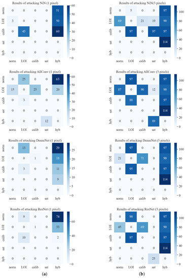
Figure 6.
Figures above show the attack efficiency of perturbing 1 pixel and 3 pixels under 2000 times non-target attacks in the same dataset. The darker color shades represent the greater number of success attacks. (a) The result of target attacks by perturbing 1 pixel of an input matrix for each network. (b) The result of target attacks by perturbing 3 pixels of an input matrix for each network. AllConv: all convolution network. NiN: Network in Network. Norm: the unattacked state. LOI: LO intensity attacks. Calib: calibration attacks. Sat: saturation attacks. Hyb: the hybrids attacks.
- Success Rate:In the case of the targeted attack, we assume a successful attack only if the adversarial example can be classified into the target class. The denominator is defined as the number of all targeted attacks we launched. In the case of the non-targeted attack, we assume a successful attack when the adversarial data can be classified into any other classes except for itself. Correspondingly, the denominator is defined as the number of adversarial examples, which is equal to a quarter of the target attack times.
- Confidence Difference:We calculate the confidence difference for each successful perturbation by subtracting the confidence of the true label after the attack from the previous confidence of the true label. At last, we take the average confidence difference of all the successful target attacks as our evaluation indicator.
- Probability of Being Attacked:We introduce a false negative (FN) to estimate the probability of a CV-QKD attack strategy being misclassified.where denotes the number of examples that belong to an certain attack type but are not identified as such a type after a non-target attack, and denotes the number of examples with the true class of i.
- Probability of Being Mistaken:To estimate the probability of a CV-QKD attack strategy being mistaken, we introduce a false positive (FP), which denotes the number of examples that do not belong to a certain attack type but are identified as such a type after a target attack.where denotes the number of target attacks with the target of i.
3.2. Analysis
Based on the 2000 times of target one-pixel attacks launched in each network, the success rate of the target attacks mainly hovers around , for AllConv , DenseNet , and ResNet . The appearance of attacking the NiN network is more arresting with a success rate of . As for the non-target attack, it shows that a success rate of attacking the NiN model reaches , while the other three models are , , and , respectively. In comparison with the original accuracy of the classification networks in Table 1, our perturbations successfully deceive all the four representative DNNs for CV-QKD attack detection.
Nevertheless, compared with the classical one-pixel attack in the image classification, it seems that the effect is not good enough. However, such a comparison is not reasonable. What is noteworthy is that, in the original CIFAR-10 test dataset, a more limited attack scenario, the original one-pixel attack also only gains , , and success rates. This result is more referential to judge the effect of our attack because our inputs have less practical noise, which obtains the target model with a higher classification accuracy. On the other hand, it also represents that our attack can achieve a better performance if the target model is trained by a more practical dataset with some real noise. The above result of our work suffices to prove the effectiveness of applying the one-pixel attack in CV-QKD attack detection networks. In the later work, we also try to increase the success rate on the basis of this scheme and successfully achieve our goal.
Table 2 shows the confidence differences of each model on average, which are , , , and . It means each successful target attack can lead to a diminution of in confidence, averagely. Since our strategy is to make the target network misclassify the perturbed data to a wrong class, the size of the numeric value does not matter, all that matters is if the attack succeeds. So, we can see that the value of confidence difference is not very high. It only represents the necessary decrement for misclassifying a CV-QKD attack.

Table 2.
Success rate, including target attack and non-target attack, and confidence difference of one-pixel attacks. AllConv: all convolution network. NiN: Network in Network. Non-tar Attack: non-target attack.
The probability of being mistaken and attacked in each class can be seen in Table 3 and Table 4. We can obviously see that the LO intensity attack strategy, calibration attack strategy, and normal condition have a high probability of being attacked, while the hybrid attack has the highest probability of being mistaken. Otherwise, the normal condition is much more vulnerable than others under one-pixel attacks. The hybrid attack is the easiest class to be disguised as. Otherwise, Figure 6a shows that the confusion matrix of each model is almost under the same distribution.

Table 3.
The probability of being mistaken under target attack (1 pixel). AllConv: all convolution network. NiN: Network in Network. Normal: the unattacked state. LOI: LO intensity attacks. Calib: calibration attacks. Sat: saturation attacks. Hyb: the hybrids attacks.

Table 4.
The probability of being attacked under non-target attack (1 pixel). AllConv: all convolution network. NiN: Network in Network. Normal: the unattacked state. LOI: LO intensity attacks. Calib: calibration attacks. Sat: saturation attacks. Hyb: the hybrids attacks.
To make a further advance in the success rate, we enlarge the number of perturbed pixels from one to three and conduct the attack on the same dataset. The results can be seen in Table 5 and Table 6 and Figure 6b. This modification gains a remarkable improvement, which enables the success rate to achieve up to success at least. Nonetheless, there is still an unattackable class for some of the models. We can see that the difference in the two possibly indicates that between difference models are smaller when carrying out a three-pixel attack. In a one-pixel attack, the difference in the train parameters and structure of the network led to the sensitivity of the minimum perturbation to have some diversity. Although, when we enlarge the perturbation, the difference between the models significantly decreases. Apart from that, the probability of being attacked can reach , which means that our adversarial attack is effective for the CV-QKD attack conditions, except for the hybrid strategy, in all of our experiments.

Table 5.
The probability of being mistaken under target attack (3 pixel). AllConv: all convolution network. NiN: Network in Network. Normal: the unattacked state. LOI: LO intensity attacks. Calib: calibration attacks. Sat: saturation attacks. Hyb: the hybrids attacks.

Table 6.
The probability of being attacked under non-target attack (3 pixel). AllConv: all convolution network. NiN: Network in Network. Normal: the unattacked state. LOI: LO intensity attacks. Calib: calibration attacks. Sat: saturation attacks. Hyb: the hybrids attacks.
3.3. Discussion
Obviously, the three advantages of the original one-pixel attack, the minimal perturbed point, semi-black box attack, and universal for most of the DNNs, can also be seen to be advantages of our migrated attack approach. To launch our adversarial attack, we only need the probability labels of the target network but not the inner parameters of a CV-QKD attack detection model. On the one hand, since we take DE as our optimization method, the problem led by calculating its gradient can be avoided. On the other hand, this optimization method allows us to apply our attack strategy in more DNNs instead of only these four networks validated by our work. Moreover, on account of modifying just one feature of the input in the same range of non-perturbed data, our adversarial examples are hard to be recognized as poisoned outlier data.
Nevertheless, as a low-cost and easy-implemented attack, it has a possibility of being detected by some adversarial perturbation detecting method. Many recent research projects put forward some countermeasures to defend against adversarial attacks, for example, the binary classifiers for distinguishing legitimate input and adversarial examples [35,36]. However, such detection layers also introduce the time delay into the CV-QKD attack detection network, which impairs the practicality to some degree. On the other hand, it is hard to show enough consideration to the intensity of the disturbance when considering the number of perturbed unites. As a result, there are some defense methods which are directly against a one-pixel attack. A patch selection denoiser [37], for example, has been proved to be efficient for a one-pixel attack, which can achieve a success rate of 98%. However, practical DNN models should take most adversarial attacks into consideration instead of just being aimed at one special attack. Such a targeted defense is not very economic. As a novel attempt at migrating adversarial attacks into the CV-QKD field, the meaning of our work is more about proving the possibility of the adversarial, not to propose a perfect attacking method. To guarantee the security of networks is a topic for a further investigation.
4. Conclusions
In this paper, we present that the one-pixel attack for deceiving the image classification network can be utilized via deceiving the CV-QKD attack detection networks. By carrying out a corresponding experimental demonstration in a simulated GMCS CV-QKD system, our results show that in four representative DNN models for CV-QKD attack detection, one-pixel attacks reach the highest success rate of , while the three others are , , and . In addition, we find an interesting appearance that the success rate of our attack can be elevated sharply up to , , , and by merely increasing the number of altered pixels to three. Furthermore, when launching a three-pixel attack, nearly of the test data from the normal state can be attacked into other attack strategies for each model, which provides the conditions for a denial of a service attack. All these consequences directly reveal the vulnerability of CV-QKD attack detection networks. Although the potential security threat brought about by using DNNs detecting CV-QKD attacks was solved, some security problems still remain.
Author Contributions
Conceptualization, Y.G.; methodology, Y.G.; resources, D.H.; software, Y.G.; validation, Y.G., P.Y. and D.H.; data curation, Y.G.; Funding acquisition, P.Y.; writing—original draft preparation, Y.G.; writing—review and editing, Y.G. and D.H.; visualization, Y.G. and P.Y.; supervision, D.H. All authors have read and agreed to the published version of the manuscript.
Funding
National College Innovation Project (2022105330245).
Institutional Review Board Statement
Not applicable.
Informed Consent Statement
Not applicable.
Data Availability Statement
The data that support the findings of this study are available from the corresponding author upon reasonable request.
Acknowledgments
The authors express appreciation to Y. Mao, H. Lou and H. Du for their pioneering research. Furthermore, we thank the reviewers of this work for their valuable comments and suggestions.
Conflicts of Interest
The authors declare no conflict of interest.
Appendix A. Data Preparation
The verification of our work is based on a hypothetical GMCS CV-QKD system, where the sender Alice is at a distance of km from the receiver Bob. The other fixed parameters are set as:, according to the standard realistic assumption for CV-QKD implementations [16,25,38]. The maximum attenuation values of Bob is selected as , while the no attenuation values is . So in the condition without attacking, the mean of Bob’s measurement results is still 0, while the variance is calculated as follows:
where depends on , the power at Bob side is set as photons per pulse with fluctuation. According to the calibrated linear relationship, is set to be 0.4 in the normal condition.
The intensity attack usually executes with the help of an intensity attenuator aimed at the beam and a general Gaussian collective attack toward the signal beam. In this way, Eve can reduce the excess noise detected by Alice and Bob to an infinitely small number, which can make Eve hide from being found. The attenuation coefficient k here is range from 0 to 1. Therefore, the variance measured by Bob in this condition is given as:
where represents the noise made by Eve’s Gaussian collective attack, N represents the variance of Eve’s EPR states, and is the shot noise under intensity attack.
With the same target to reduce the detectable excess noise, the calibration attack achieves its goal by modifying the shape of pulses and intercepting a fraction of the signal pulse, implementing together with partial intercept-resent (PIR) attacks. The variance and shot noise under calibration attack is modified as
where is the excess noise introduced by PIR attack, and a typical value of .
In the saturation attack, Eve capitalizes on the finite linearity domain of the homodyne detection response to saturate Bob’s detector by doing the PIR attack and replacing the quadrature coherent states received by Bob with a replacement value . As the result, the mean and variance of Bob under saturation attack will change into the following expressions:
where , parameters A, B, C and error function are defined as
As for the hybrid attack composed of the intensity attack and wavelength attack, Eve executes an intercept-resend attack and prepares new signal and pulses in the first step. Then it resends two extra coherent pulses which have different wavelengths from the typical communication wavelength in order to ensure the shot noise measured value normal. Thus, the Bob’s measurement variance, shot noise, and excess noise can be described as:
where D corresponds to the intensities , and wavelengths , of the two extra pulses.
Appendix B. Structure of Classification Models
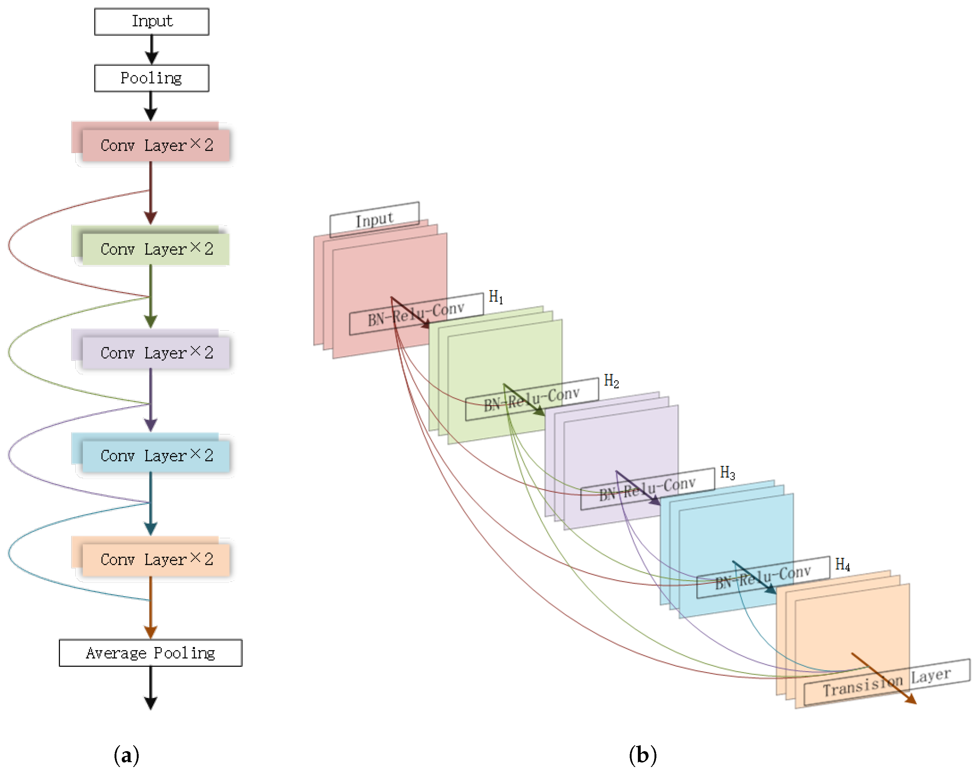
Convolutional Neural Network (CNN) was first proposed over 30 years ago. Restricted by computer hardware and network structure, the truly deep CNNs finally come into substantial real-world usage in the recent decade. In the beginning, CNN is composed of pure convolutional layers and pooling layers. As CNNs become increasingly deep, new structures are put forward in order to solve the problems of accuracy degradation and overfitting. In 2014, a novel deep network called Network In Network (NiN) [31] was proposed by Min Lin et al. to resolve the problem of overfitting. In 2015, Kaiming He et al. introduce the residual functions to reformulate the layers and present the structure of ResNet [33], shown in Figure A1a, which shows excellent efficiency in image detection. A few years later in 2018, Gao Huang et al. propose the Dense Convolutional Network (DenseNet) [34], which connects each layer to every other layer in a way of feed-forward, shown in Figure A1b. It shows a better performance with less number of parameters.
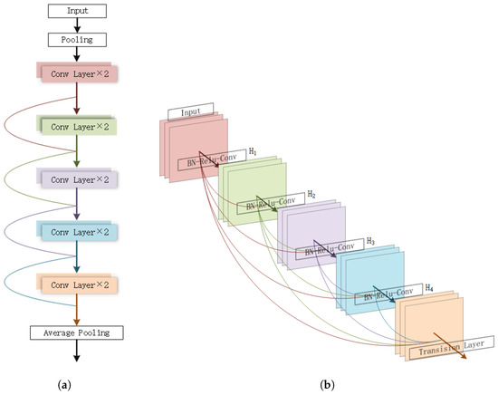
Figure A1.
Above figures show the main structure of DenseNet and ResNet. (a) The framework of a 10 convolutional layers ResNet as sketchy plot. (b) A 5 layers dense block with a growth rate of . The DenseNet in our work is consist of 3 dense block like this with different layers.
Figure A1.
Above figures show the main structure of DenseNet and ResNet. (a) The framework of a 10 convolutional layers ResNet as sketchy plot. (b) A 5 layers dense block with a growth rate of . The DenseNet in our work is consist of 3 dense block like this with different layers.
The classical networks above, NiN, ResNet, and DenseNet, are the basic structure we used in our work. As a method to fit a fonctionelle, DNN is also effective outside the field of image processing in theory and practice. Considering the characteristics of the measured data in CV-QKD attack detection, we set up our network with a relatively simple structure. In our work, the NiN is set to be 9 convolutional layers and 3 pooling layers. In addition, we choose the 34 layers architecture for ResNet and 50 layers for DenseNet. The learning rate of the training decrease from to with the growth of training epochs. After our testing, the optimum training epochs and batch size of these four detection networks are shown in Table 1.
References
- Scarani, V.; Bechmann-Pasquinucci, H.; Cerf, N.J.; Dušek, M.; Lütkenhaus, N.; Peev, M. The security of practical quantum key distribution. Rev. Mod. Phys. 2009, 81, 1301. [Google Scholar] [CrossRef]
- Gisin, N.; Ribordy, G.; Tittel, W.; Zbinden, H. Quantum cryptography. Rev. Mod. Phys. 2002, 74, 145. [Google Scholar] [CrossRef]
- Weedbrook, C.; Pirandola, S.; García-Patrón, R.; Cerf, N.J.; Ralph, T.C.; Shapiro, J.H.; Lloyd, S. Gaussian quantum information. Rev. Mod. Phys. 2012, 84, 621. [Google Scholar] [CrossRef]
- Xu, F.; Curty, M.; Qi, B.; Qian, L.; Lo, H.K. Discrete and continuous variables for measurement-device-independent quantum cryptography. Nat. Photonics 2015, 9, 772–773. [Google Scholar] [CrossRef]
- Bennett, C.H. Quantum cryptography using any two nonorthogonal states. Phys. Rev. Lett. 1992, 68, 3121. [Google Scholar] [CrossRef] [PubMed]
- Grosshans, F.; Grangier, P. Continuous variable quantum cryptography using coherent states. Phys. Rev. Lett. 2002, 88, 057902. [Google Scholar] [CrossRef]
- Huang, D.; Huang, P.; Lin, D.; Zeng, G. Long-distance continuous-variable quantum key distribution by controlling excess noise. Sci. Rep. 2016, 6, 19201. [Google Scholar] [CrossRef] [PubMed]
- Leverrier, A.; Grangier, P. Unconditional security proof of long-distance continuous-variable quantum key distribution with discrete modulation. Phys. Rev. Lett. 2009, 102, 180504. [Google Scholar] [CrossRef] [PubMed]
- Cao, Y.; Zhao, Y.; Wang, Q.; Zhang, J.; Ng, S.X.; Hanzo, L. The evolution of quantum key distribution networks: On the road to the qinternet. IEEE Commun. Surv. Tutor. 2022, 24, 839–894. [Google Scholar] [CrossRef]
- Grosshans, F.; Van Assche, G.; Wenger, J.; Brouri, R.; Cerf, N.J.; Grangier, P. Quantum key distribution using gaussian-modulated coherent states. Nature 2003, 421, 238–241. [Google Scholar] [CrossRef]
- Leverrier, A.; Karpov, E.; Grangier, P.; Cerf, N.J. Security of continuous-variable quantum key distribution: Towards a de Finetti theorem for rotation symmetry in phase space. New J. Phys. 2009, 11, 115009. [Google Scholar] [CrossRef]
- Furrer, F.; Franz, T.; Berta, M.; Leverrier, A.; Scholz, V.B.; Tomamichel, M.; Werner, R.F. Continuous variable quantum key distribution: Finite-key analysis of composable security against coherent attacks. Phys. Rev. Lett. 2012, 109, 100502. [Google Scholar] [CrossRef]
- Leverrier, A. Security of continuous-variable quantum key distribution via a Gaussian de Finetti reduction. Phys. Rev. Lett. 2017, 118, 200501. [Google Scholar] [CrossRef]
- Huang, J.Z.; Weedbrook, C.; Yin, Z.Q.; Wang, S.; Li, H.W.; Chen, W.; Guo, G.C.; Han, Z.F. Quantum hacking of a continuous-variable quantum-key-distribution system using a wavelength attack. Phys. Rev. A 2013, 87, 062329. [Google Scholar] [CrossRef]
- Ma, X.C.; Sun, S.H.; Jiang, M.S.; Liang, L.M. Wavelength attack on practical continuous-variable quantum-key-distribution system with a heterodyne protocol. Phys. Rev. A 2013, 87, 052309. [Google Scholar] [CrossRef]
- Jouguet, P.; Kunz-Jacques, S.; Diamanti, E. Preventing calibration attacks on the local oscillator in continuous-variable quantum key distribution. Phys. Rev. A 2013, 87, 062313. [Google Scholar] [CrossRef]
- Ma, X.C.; Sun, S.H.; Jiang, M.S.; Liang, L.M. Local oscillator fluctuation opens a loophole for Eve in practical continuous-variable quantum-key-distribution systems. Phys. Rev. A 2013, 88, 022339. [Google Scholar] [CrossRef]
- Qin, H.; Kumar, R.; Alléaume, R. Quantum hacking: Saturation attack on practical continuous-variable quantum key distribution. Phys. Rev. A 2016, 94, 012325. [Google Scholar] [CrossRef]
- Qin, H.; Kumar, R.; Makarov, V.; Alléaume, R. Homodyne-detector-blinding attack in continuous-variable quantum key distribution. Phys. Rev. A 2018, 98, 012312. [Google Scholar] [CrossRef]
- Pirandola, S.; Ottaviani, C.; Spedalieri, G.; Weedbrook, C.; Braunstein, S.L.; Lloyd, S.; Gehring, T.; Jacobsen, C.S.; Andersen, U.L. High-rate measurement-device-independent quantum cryptography. Nat. Photonics 2015, 9, 397–402. [Google Scholar] [CrossRef]
- Lo, H.K.; Curty, M.; Qi, B. Measurement-device-independent quantum key distribution. Phys. Rev. Lett. 2012, 108, 130503. [Google Scholar] [CrossRef]
- Xu, F.; Ma, X.; Zhang, Q.; Lo, H.K.; Pan, J.W. Secure quantum key distribution with realistic devices. Rev. Mod. Phys. 2020, 92, 025002. [Google Scholar] [CrossRef]
- Zhang, C.; Lu, Y. Study on artificial intelligence: The state of the art and future prospects. J. Ind. Inf. Integr. 2021, 23, 100224. [Google Scholar] [CrossRef]
- Huang, D.; Liu, S.; Zhang, L. Secure Continuous-Variable Quantum Key Distribution with Machine Learning. Photonics 2021, 8, 511. [Google Scholar] [CrossRef]
- Mao, Y.; Huang, W.; Zhong, H.; Wang, Y.; Qin, H.; Guo, Y.; Huang, D. Detecting quantum attacks: A machine learning based defense strategy for practical continuous-variable quantum key distribution. New J. Phys. 2020, 22, 083073. [Google Scholar] [CrossRef]
- Luo, H.; Zhang, L.; Qin, H.; Sun, S.; Huang, P.; Wang, Y.; Wu, Z.; Guo, Y.; Huang, D. Beyond universal attack detection for continuous-variable quantum key distribution via deep learning. Phys. Rev. A 2022, 105, 042411. [Google Scholar] [CrossRef]
- Du, H.; Huang, D. Multi-Attack Detection: General Defense Strategy Based on Neural Networks for CV-QKD. Photonics 2022, 9, 177. [Google Scholar] [CrossRef]
- Yuan, X.; He, P.; Zhu, Q.; Li, X. Adversarial examples: Attacks and defenses for deep learning. IEEE Trans. Neural Netw. Learn. Syst. 2019, 30, 2805–2824. [Google Scholar] [CrossRef]
- Su, J.; Vargas, D.V.; Sakurai, K. One pixel attack for fooling deep neural networks. IEEE Trans. Evol. Comput. 2019, 23, 828–841. [Google Scholar] [CrossRef]
- Das, S.; Suganthan, P.N. Differential evolution: A survey of the state-of-the-art. IEEE Trans. Evol. Comput. 2010, 15, 4–31. [Google Scholar] [CrossRef]
- Lin, M.; Chen, Q.; Yan, S. Network in network. arXiv 2013, arXiv:1312.4400. [Google Scholar]
- Simonyan, K.; Zisserman, A. Very deep convolutional networks for large-scale image recognition. arXiv 2014, arXiv:1409.1556. [Google Scholar]
- He, K.; Zhang, X.; Ren, S.; Sun, J. Deep residual learning for image recognition. In Proceedings of the IEEE Conference on Computer Vision and Pattern Recognition, Las Vegas, NV, USA, 27–30 June 2016; pp. 770–778. [Google Scholar]
- Huang, G.; Liu, Z.; Van Der Maaten, L.; Weinberger, K.Q. Densely connected convolutional networks. In Proceedings of the IEEE Conference on Computer Vision and Pattern Recognition, Honolulu, HI, USA, 21–26 July 2017; pp. 4700–4708. [Google Scholar]
- Lu, J.; Issaranon, T.; Forsyth, D. Safetynet: Detecting and rejecting adversarial examples robustly. In Proceedings of the IEEE International Conference on Computer Vision, Venice, Italy, 22–29 October 2017; pp. 446–454. [Google Scholar]
- Bhagoji, A.N.; Cullina, D.; Mittal, P. Dimensionality reduction as a defense against evasion attacks on machine learning classifiers. arXiv 2017, arXiv:1704.02654. [Google Scholar]
- Chen, D.; Xu, R.; Han, B. Patch selection denoiser: An effective approach defending against one-pixel attacks. In Proceedings of the International Conference on Neural Information Processing, Sydney, NSW, Australia, 12–15 December 2019; pp. 286–296. [Google Scholar]
- Fossier, S.; Diamanti, E.; Debuisschert, T.; Villing, A.; Tualle-Brouri, R.; Grangier, P. Field test of a continuous-variable quantum key distribution prototype. New J. Phys. 2009, 11, 045023. [Google Scholar] [CrossRef]
Disclaimer/Publisher’s Note: The statements, opinions and data contained in all publications are solely those of the individual author(s) and contributor(s) and not of MDPI and/or the editor(s). MDPI and/or the editor(s) disclaim responsibility for any injury to people or property resulting from any ideas, methods, instructions or products referred to in the content. |
© 2023 by the authors. Licensee MDPI, Basel, Switzerland. This article is an open access article distributed under the terms and conditions of the Creative Commons Attribution (CC BY) license (https://creativecommons.org/licenses/by/4.0/).


