High-Flux Fast Photon-Counting 3D Imaging Based on Empirical Depth Error Correction

Abstract

The time-correlated single-photon-counting (TCSPC) three-dimensional (3D) imaging lidar system has broad application prospects in the field of low-light 3D imaging because of its single-photon detection sensitivity and picoseconds temporal resolution. However, conventional TCSPC systems always limit the echo photon flux to an ultra-low level to obtain high-accuracy depth images, thus needing to spend amounts of acquisition time to accumulate sufficient photon detection events to form a reliable histogram. When the echo photon flux is increased to medium or even high, the data acquisition time can be shortened, but the photon pile-up effect can seriously distort the photon histogram and cause depth errors. To realize high accuracy TCSPC depth imaging with a shorter acquisition time, we propose a high-flux fast photon-counting 3D imaging method based on empirical depth error correction. First, we derive the photon flux estimation formula and calculate the depth error of our photon-counting lidar under different photon fluxes with experimental data. Then, a function correction model between the depth errors and the number of echo photons is established by numerical fitting. Finally, the function correction model is used to correct depth images at high photon flux with different acquisition times. Experimental results show that the empirical error correction method can shorten the image acquisition time by about one order of magnitude while ensuring a moderate accuracy of the depth image.

1. Introduction

Three-dimensional (3D) imaging technology based on time-correlated single photon-counting (TCSPC) lidar has single-photon detection sensitivity and picoseconds time resolution, which can be used to obtain fine surface topography of the target at very low illumination laser power or to obtain images of long-distance targets [1,2,3]. It has broad application prospects in underwater target detection [4,5,6], remote sensing [7], and other 3D imaging fields [8,9,10,11].

High-accuracy depth imaging with fast acquisition time is one of the main goals pursued by 3D imaging technology. Through repeated illumination of a short laser pulse and detecting echo photons with detectors such as the single-photon avalanche diode (SPAD) connected to precision timing electronics, the TCSPC system can build up a histogram of photon detection times relative to the illumination time that implies high-precision time-of-flight (TOF) information of the laser pulse. Although the TCSPC 3D imaging system can acquire 3D images with high depth accuracy based on its unique TOF measurement ability, the long image acquisition time still limits its practical application in many scenarios. The main reason for the long acquisition time of the TCSPC 3D imaging lidar system is that typical TCSPC adopts an extremely low photon flux regime to avoid the photon pile-up distortion caused by the dead time of the detector and TCSPC timing electronics [12,13]. During one cycle, once a photon is detected, the subsequently arrived photons will not be recorded by the detector, so that the photon-counting histogram undergoes so-called pile-up distortion [14,15]. This distortion will lead to an inaccurate TOF measurement, corresponding to an inaccurate depth measurement. Therefore, conventional TCSPC 3D imaging systems always limit the laser power to keep the average number of detected photons in a period much less than 1 (typically below 0.05) to avoid distortion [16], i.e., they operate in the low-flux regime. Therefore, it requires long acquisition times, even hours and days, to ensure that sufficient photons are detected at each pixel to obtain a highly accurate 3D image of the target in a low-flux regime [17,18].

Previous research works aiming to realize fast and accurate TCSPC 3D imaging can be divided into two main categories, including improving hardware and developing advanced data-processing algorithms. In Refs. [12,19], dead time was reduced with the new detector structure as well as with optimized TCSPC electronics. However, the development of the new detector is still in the laboratory stage and there is also typically a trade-off between the dead time and the minimum time-bin duration of the TCSPC electronics [12]. In Ref. [20], Ye et al. proposed a method to improve the ranging accuracy based on the dual SPAD detector structure, with two detection channels corresponding to strong and weak echoes, respectively. Although this method can improve the depth accuracy, they found that it had limited effects when there was a large fluctuation of echo photon flux. In Ref. [21] a probability distribution regulator method was proposed to ensure the fixed number of photon incidents on the SPAD by adjusting the emitted laser power to restrain the depth error, but the feedback and response speed of the regulator still need to be improved. In terms of the development of data processing methods, Oh et al. [22] presented a method based on the SPAD detection probability theoretical model to reduce the depth error. He et al. [23] proposed a method based on the functional relationship between the depth error and the laser pulse response rate. Xu et al. [24] proposed a method consisting of a recursive signal processing technique based on the Poisson probability response model to recover the underlying distribution of echo photons. However, they all just focused on the restraint of depth error rather than the imaging time efficiency. Felix Heide et al. [17] proposed a probabilistic imaging model suitable for low flux to high flux, accurately modeling the pile-up deformation problem in the model, using a statistical priors and inverse method to derive depth and reflectivity images and enabling 3D imaging with sub-picosecond accuracy. Differing from Ref. [17], Joshua Rapp et al. [18] aimed at dead time compensation for lidar working with an asynchronous TCSPC mode, which is common in lidars combining free-running SPADs and modern TCSPC. They proposed a Markov chain detection probability model suitable for high flux and an algorithm to correct the detection histogram distortion caused by dead time. An average of up to five photons per illumination cycle was achieved, improving the acquisition time by two orders of magnitude. The above two methods shorten the acquisition time through a high-flux regime and obtain high depth accuracy, but they introduce complex probability models and algorithms, which lead to high computation costs.

In this paper, an empirical depth error correction method is used to realize fast photon-counting 3D imaging at high flux. The data acquisition time is shortened by the high-flux regime, and the depth estimation error caused by photon pile-up is quickly corrected by an empirical correction without high computation cost. The experimental results show that the empirical error correction method can shorten the image acquisition time by about one order of magnitude while ensuring moderate imaging accuracy, which is more suitable for practical engineering applications.

2. Depth Error Correction Method

The impact of the incident photons on the active area of the SPAD detector causes an avalanche of electronic carriers, which produces a detectable current pulse signal. Then, the current must be quenched to reset the detector to a photon-sensitive state and keep the detector off for a few tens of nanoseconds (hold-off time) to avoid the influence of the after-pulse probability. Therefore, no new photon arrival event can be detected during the quenching time and hold-off time, the sum of which is called the dead time of the detector. Here, we assume that the avalanche trigger probability is approximately 1, i.e., any echo photon converted to a photoelectron will cause an avalanche if it is not within the detector’s dead time. Feller divided detectors into non-paralyzed detectors and paralyzed detectors based on their paralyzability [25]. In this work, we only consider non-paralyzed detectors that are dead within a fixed time after detection, regardless of whether additional photons arrive during the dead time. The dead time of the detector and timing device is collectively referred to as the TCSPC system dead time. We assume that the SPAD is fully quenched between successive laser pulses, and that the end of the system’s dead time synchronizes with the beginning of the illumination cycle, i.e., each emitted laser pulse produces at most one detected photon event. As mentioned above, the fluctuation of echo photon flux (i.e., the average number of echo photons per pulse) affects depth measurement accuracy due to the dead time of the TCSPC system. Different reflectivity or distance of each pixel in real scenes will cause large fluctuations in echo intensity, resulting in large errors in depth imaging results. Therefore, we first model the photon detection process and derive the echo photon flux estimation formula. Then, the depth error function correction model of the detection system is established by experimental data. Finally, the analysis for time efficiency and imaging accuracy of the empirical error correction method is described in Section 3.

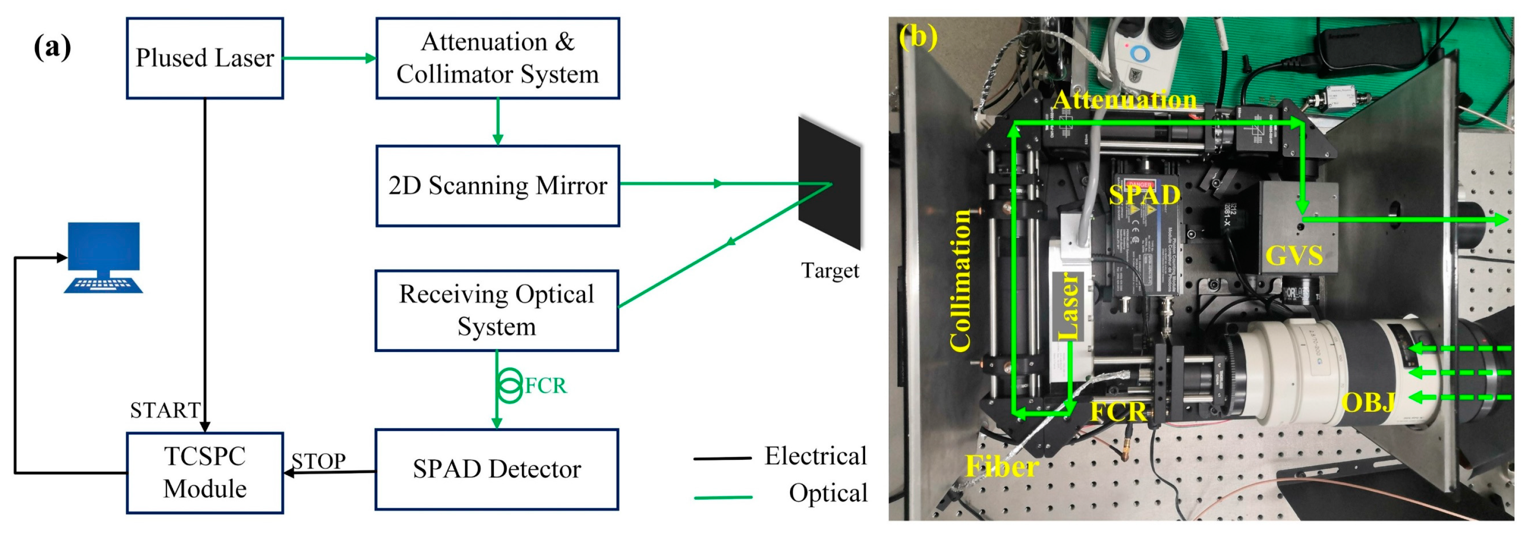
2.1. Experimental Setup

The schematic diagram and physical photograph of our TCSPC 3D imaging system are shown in Figure 1. The illumination source is a 532 nm pulsed laser (Teemphotonics, SNG-20F-100, Meylan, FR), with a pulse width of fewer than 750 picoseconds and a pulse repetition rate of 21.2 kHz. The optical collimation mode consists of two lenses with focal lengths of 25.4 mm and 125 mm, making the divergence angle of the emission laser beam less than 2 mrad. Through the adjustable attenuator, composed of two polarization beam splitters and one half-wave plate, the output laser power can be adjusted from 0.5 μW~28 mW. The receiving objective system consists of a Φ78 mm objective lens (SONY, SAL70200G, TYO, JP), a 35 mm focal length eyepiece, and a band pass filter (BPF) (Thorlabs, FL532-1, Newton, NJ, USA) with a bandwidth of 1 nm and a center wavelength of 532 nm. The beam-scanning galvanometer (Thorlabs, GVS212M, Newton, NJ, USA) has a beam allowable size of 10 mm and a maximum scanning angle of ±20°. The collected echo photons are transmitted to the SPAD through a fiber coupler (Thorlabs, F220FC-532) and multimode fiber (Thorlabs, M31L01) with a core size of 62.5 μm. The optical axis of the outgoing laser is approximately parallel to the optical axis of the receiving optical system. The SPAD detector from Excelitas corporation (SPCM-AQRH-16, East Waltham, MA, USA) provides a photon detection efficiency of about 55% at 532 nm, with a Φ180 μm active area, a ~350 ps timing jitter, a 35 ns dead time, and a ~25 Hz dark count rate. The photon arrival time is recorded by a TCSPC module of HydraHarp400 with an 80 ns dead time. Its time-bin size is set to 4 ps during the experiment.

2.2. Probabilistic Detection Model and Derivation of Echo Photon Flux

In our system, the SPAD and TCSPC dead times are 35 ns and 80 ns, respectively, while the period of the laser pulse is 47.2 μs, that is, the pulse period is much longer than the dead time of the TCSPC system. Therefore, it is assumed that each of the N laser pulses is an independent measurement. The photon detection process will be discussed by taking a single pixel as an example. Conventional 3D imaging methods always make the SPAD detector in the low-flux regime, in which the dead time of the system can be ignored, and the Poisson process is used to model the number of photons arriving in a time bin. For the measurement of medium and high fluxes, the dead time of the system cannot be ignored. Due to the dead time, arriving photons are more likely to be recorded in the earlier bins than in the later bins, and the photon is recorded in bin $i$ only if no arriving photon is detected in the previous $i-1$ bins. The probability $P\left(h|\lambda \right)$ of detecting the histogram $h$ is given by the multinomial distribution [17]:

$$\begin{array}{l}P\left(h|\lambda \right)=\frac{N!}{h_1!\cdots h_T!\left(N-1^{T}h\right)!}\cdot P{\left(\mathrm{no}\mathrm{detections}\right)}^{N-1^{T}h}\cdot {{\displaystyle \prod _{i=1}^{T}P\left(i|\lambda \right)}}^{h_i}\\ =\frac{N!}{h_1!\cdots h_T!\left(N-1^{T}h\right)!}\cdot \exp {\left(-1^T\lambda \right)}^{N-1^{T}h}\cdot {{\displaystyle \prod _{i=1}^T\left(\exp \left(-{\displaystyle \sum _{k=1}^{i-1}{\lambda }_k}\right)-\exp \left(-{\displaystyle \sum _{k=1}^i{\lambda }_k}\right)\right)}}^{h_i}\end{array},$$

(1)

where $N$ denotes the total number of pulses emitted, $h_i$ denotes the accumulated counts in bin $i$ over the $N$ emitted pulses, $h$ denotes the photon count vector of the entire histogram, $T$ denotes the number of time bins, ${\lambda }_i$ denotes the Poisson rate for the number of detections in bin $i$, $\lambda$ denotes the Poisson rate vector of the entire histogram, and $1$ denotes a vector with all entries equal to one.

By performing a maximum likelihood estimation on Equation (1), ${\lambda }_i$ can be obtained by Equation (2) [17]:

$${\stackrel{⌢}{\lambda }}_i=-\log \left(1-h_i/\left(N-{\displaystyle \sum _{k=1}^{i-1}{h}_k}\right)\right) \forall i\in \left\{1,\cdots ,T\right\}.$$

(2)

Then, the average photon number $N_{\mathrm{s}}$ per pulse can be calculated by summing ${\stackrel{⌢}{\lambda }}_i$, denoted as Equation (3), where $N_{\det }={\displaystyle \sum _{k=1}^T{h}_k}$ represents the total number of photon detections over the histogram $h$,

$$N_{\mathrm{s}}={\stackrel{⌢}{\lambda }}_1+{\stackrel{⌢}{\lambda }}_2+\cdots {\stackrel{⌢}{\lambda }}_T=-\left\{\log \frac{N-h_1}{N}+\log \frac{N-{\displaystyle \sum _{k=1}^2{h}_k}}{N-h_1}+\cdots +\log \frac{N-{\displaystyle \sum _{k=1}^T{h}_k}}{N-{\displaystyle \sum _{k=1}^{T-1}{h}_k}}\right\}=-\log \left(1-\frac{N_{\det }}{N}\right).$$

(3)

The ratio of the number of detections to the number of fired laser pulses ($\frac{N_{\det }}{N}$) is also known as the laser pulse response rate or detection rate [23].

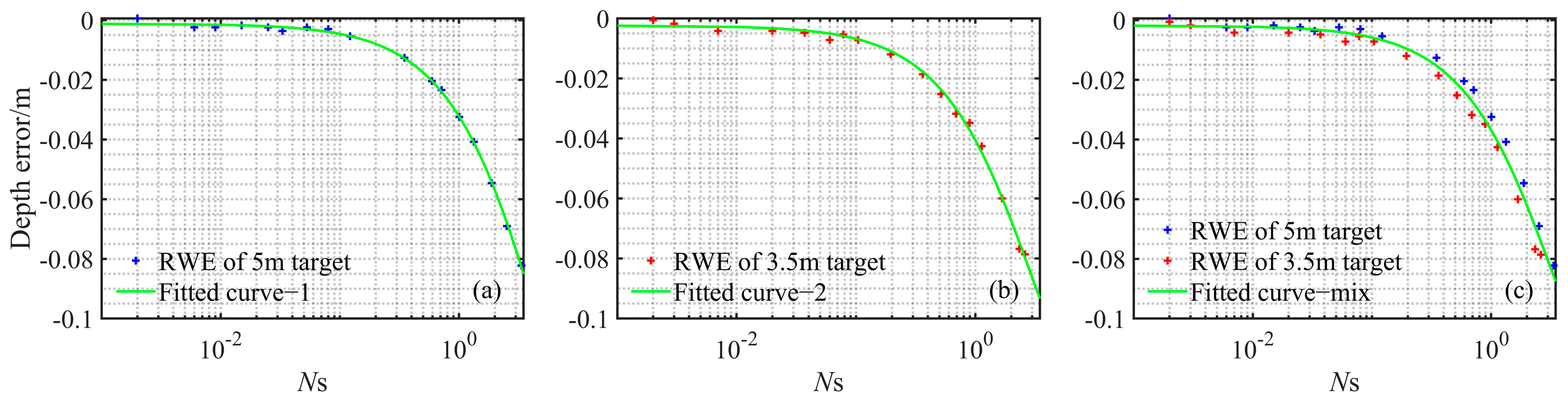
2.3. Depth Error Function Correction Model

In order to establish the depth error function correction model, i.e., the relationship between the depth error and the average photon number under different echo intensities, a series of photon count histograms were obtained on targets at two different distances. Then, the empirical depth error function correction model, which is independent of the target’s distance and only related to the echo photon number, was obtained by numerical fitting of depth error values.

The detailed experimental steps are as follows. First, we respectively measure the truth value under low flux for the targets at distances of 3.5 m and 5 m. Second, we measure the photon count histogram under a series of different illumination intensities (corresponding detection rate range of 2~97%, and $N_{\mathrm{s}}$ from 0.002~3.349). The cross-correlation algorithm is used to calculate the depth value from the measured photon counting histograms. Then, two groups of depth error data, varying with the number of echo photons, are obtained by subtracting the ground-truth depth value from the measured depth values. After that, the two groups depth error data of targets and their mixed depth error data are shown in Figure 2a–c. Finally, according to the trend of depth error changing with the number of echo photons [23,26], the function model $f_{err}\left(N_s\right)=a\times e^{-b\times N_s}+c$ is used to numerically fit the relationship between the depth error $f_{\mathrm{err}}$ and photon number $N_{\mathrm{s}}$. Parameters are fitted as a = 0.1554, b = 0.2222 and c = −0.1566 in Figure 2a, a = 0.1285, b = 0.3525 and c = −0.1309 in Figure 2b, a = 0.1267, b = 0.3234 and c = −0.1285 in Figure 2c, respectively. The function correction model is shown by the green line in Figure 2a–c and the calculated depth error from experimental data is marked by blue and red plus symbols.

3. Experimental Results and Analysis

To analyze the depth image accuracy and time efficiency of the depth error correction method, we carried out depth imaging experiments for targets 5 m away under low-flux and high-flux conditions by adjusting the output laser power. The depth image with 50 × 50 pixels was acquired under different acquisition times. In a low-flux regime, we set a group of total acquisition times (160 s, 400 s, 800 s, 1200 s, 1600 s, 2000 s, 3200 s, and 4000 s) to analyze time efficiency. In a high-flux regime, the total acquisition times were set relatively short, at 10 s, 20 s, 30 s, 40 s, 50 s, 80 s, and 100 s, since sufficient photons could be obtained with a short acquisition time at high flux. Last, we also validated the image correction performance of the proposed method under high-flux conditions by placing targets at a distance of 10 m.

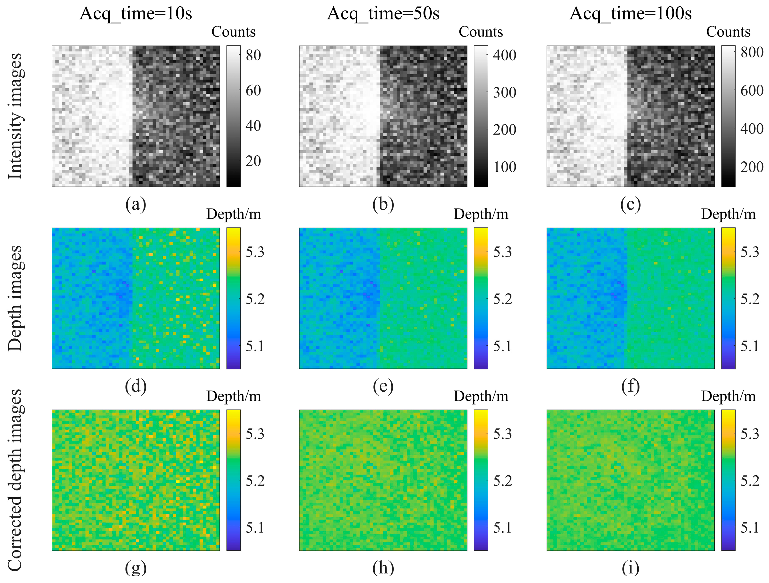
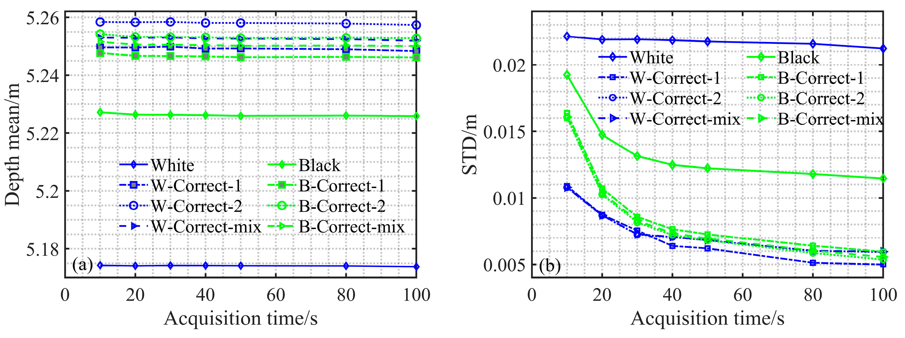
3.1. Depth Imaging Experiment for a White-Black Plate Target

Figure 3a shows a white–black plate target, which consists of two areas with the same depth but different reflectivity. The left side of the target is white and the right side is black. The size of the laser scanning area is 12 cm × 12 cm. The distance between the target and the imaging system is more than 5 m. If the laser beam is incident perpendicular to the center of the target plate, then all scan points on the plate can be considered to have almost the same depth value.

Figure 3b,c show the intensity image and depth image of the target at low flux with a long time acquisition of 4000 s. The average numbers of photons per pulse per pixel are calculated as 0.029 in the white area and 0.006 in the black area using Equation (3), which meets the requirement of a low-flux regime ($N_{\mathrm{s}}$ < 0.05). As can be seen from the depth image in Figure 3c, although the depth values of the black area on the right side fluctuate more seriously than those of the white area on the left side, due to less photon accumulation, the depth bias between the two sides is not obvious. Figure 3d shows the depth histograms for the black and white areas. The two depth histograms overlapped well, proving that the depth bias is basically negligible at low flux conditions. It can also be seen that the depth histogram of the white area, with higher reflectivity, has a narrower width than that of the black area. It means that the depth precision of the white area is higher than that of the black area, which is consistent with the result observed in Figure 3c.

Figure 4 shows the mean values and standard deviations (STD) of the depth image in the black and white areas under different acquisition times to quantitatively evaluate the depth-imaging accuracy. As can be seen from Figure 4a, the mean depth tends to be stable with the increase in acquisition time, and the mean values are stable at 5.2446 m and 5.2421 m for the black and white areas, respectively. The tiny bias might be due to the SPAD’s time-walk effect under different photon-count rates, even in low photon flux [27]. As can be seen from Figure 4b, the STD gradually decreases as the acquisition time increases. This is because longer acquisition times can accumulate more photons, resulting in optimized depth precision. Finally, when the acquisition time was increased to 4000 s, the STD of the black area and white area stabilized at 7.2 mm and 3.6 mm, respectively. Under the same acquisition time, the white area can accumulate more photons due to its high reflectivity and has better depth precision.

Figure 5 shows the intensity images, depth images, and corrected depth images acquired at high flux, with short acquisition times of 10 s, 50 s, and 100 s. The average numbers of photons per pulse per pixel are calculated as 2.930 in the white area and 0.574 in the black area, which can be considered as a high-flux regime. As can be seen from the intensity image in Figure 5a–c, the accumulated photon counts increase as the acquisition time. Figure 5d–f show the depth images obtained directly under high-flux conditions; it can be seen that the black area and white area exhibit an obvious depth bias. Figure 5g–i show the corrected depth images (using the depth error function correction model fitted curve mix in Figure 2c); it can be seen that the two areas with different reflectivity are in the same plane with the depth bias restrained well.

To evaluate the depth image accuracy and time efficiency quantitatively, the mean and STD values of the depth image in the black and white areas under different acquisition times are shown in Figure 6. From the mean depth curves in Figure 6a we see that the mean depth was virtually unaffected by the acquisition time in the current acquisition time range (10 s~100 s). The mean depth was mainly affected by the target’s reflectivity, that is, by the number of echo photons. When the acquisition time was 100 s, the depth measurement bias between black and white areas in the same plane was up to 52.1 mm. After correcting the images using the three function correction models in Figure 2a–c, the depth bias between the two areas was reduced to 2.1 mm, 4.4 mm, and 1.8 mm, respectively. Regardless of the function correction model, the depth bias between the two plane areas was reduced by at least 10 times compared with the bias before the correction. From the STD curve in Figure 6b we see that the STDs first decrease and then stabilize with the increase in acquisition time. When the acquisition time was 100 s, the STDs of the black and white areas before correction were 11.5 mm and 21.2 mm, respectively.However, the STDs corrected by the model in Figure 2a–c were reduced to 5.9 mm/5.0 mm, 5.4 mm/5.9 mm, and 5.6 mm/6.0 mm, respectively, which shows that the accuracy has been significantly improved. Compared with the depth precision under the low-flux conditions in Figure 4, the depth precision result of the black area was better than that of the low-flux 4000 s acquisition time (i.e., 7.2 mm). And the depth precision for the white area was close to the result at the low-flux with 1200 s acquisition time (i.e., 5.4 mm). In summary, the depth error function correction model mentioned in Section 2.3, which is independent of the target’s distance and only related to the number of echo photons, is proved to be effective. By correction, the acquisition time is greatly reduced by about an order of magnitude, while maintaining accuracy and precision comparable to low-flux depth imaging. This is helpful for achieving fast TCSPC 3D imaging. Meanwhile, we see that the function correction model that mixes the error data in Figure 2c can obtain higher accurate depth images than the other two models in Figure 2a,b.

Table 1. Time efficiency and accuracy analysis for depth images of the black-white plate target.

	Area	Depth Mean/Time		ΔDepth (DB−DW)	STD/Time
Low flux	Black	5.2446 m	4000 s	2.5 mm	7.2 mm	4000 s
	White	5.2421 m	4000 s		5.4 mm	1200 s
High flux	Black	5.2259 m	100 s	52.1 mm	11.5 mm	100 s
	White	5.1738 m	100 s		21.2 mm	100 s
High flux corrected	Black	5.2501 m	100 s	−1.8 mm	5.6 mm	100 s
	White	5.2519 m	100 s		6.0 mm	100 s

lists the detailed results of the time efficiency and accuracy analysis of depth images by the function correction model in Figure 2c under low- and high-flux regimes.

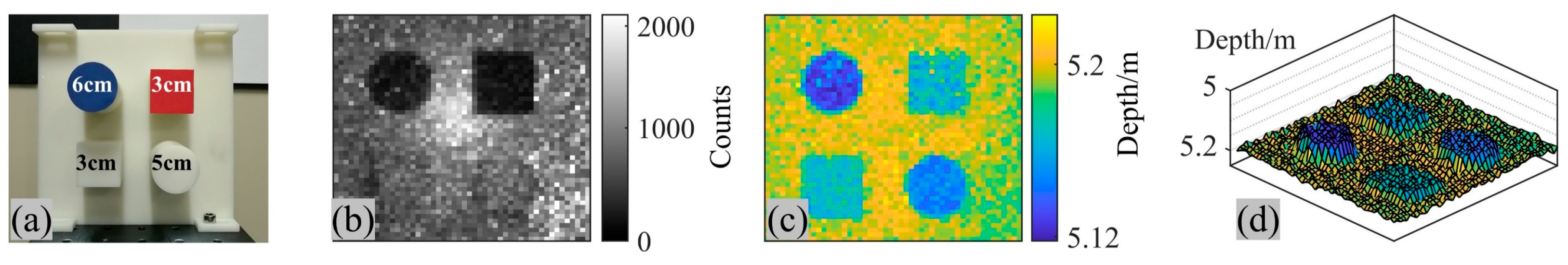
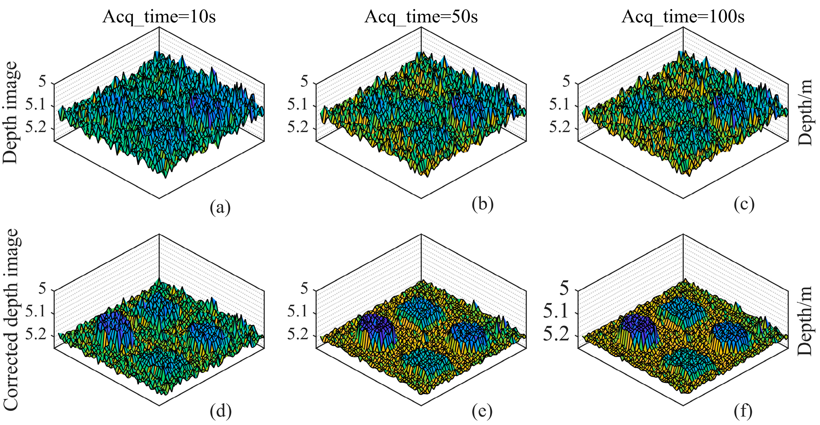
3.2. Depth Imaging Experiment for a Complex Geometry Target

To further verify the depth image accuracy and time efficiency of the error correction method, another, 3D-printed, and more complex geometry target is selected as the imaging target, shown in Figure 7a. The length and width of the whole target are both 15 cm in size. The target is mainly composed of two square pillars and two cylinders. The two square pillars are both 3 cm in height and their reflectivity is different. The reflectivity of the two cylinders is different and their heights are also different. The height of the two cylinders is 5 cm and 6 cm, as marked in Figure 7a. Figure 7b shows the intensity image of the target at low flux with a long time acquisition of 4000 s. The average number of photons per pulse per pixel is calculated as 0.023 in the whole target area. Figure 7c,d show the depth image in 2D and 3D coordinates, respectively. We can intuitively see that the depths of the two square pillars are the same, and the cylinder at top left appears closer than the cylinder at right bottom. It is actually consistent with the real geometry target, proving that depth imaging is reliable under low-flux conditions.

Figure 8 shows the depth images and corrected depth images of the complex geometry target acquired at high flux, with short acquisition times of 10 s, 50 s, and 100 s. The average number of photons per pulse per pixel is calculated as 2.599 in the whole target area, which can be considered a high-flux regime. Figure 8a–c show the depth images obtained directly at high flux. We see that all four pillars can hardly be distinguished. On the contrary, from the depth images shown in Figure 8d–f corrected with the function correction model in Figure 2c, we can easily identify the four pillars. It proves that the accuracy of the depth image is improved through correction. We also see that the imaging depth resolution is improved as well. Before correction, the cylinder with a height of 6 cm can hardly be distinguished in Figure 8a–c, while after correction, two cylinders with a minimum distance of 1 cm can be distinguished in Figure 8e,f.

The time efficiency and accuracy analysis results of depth images in four regions obtained in low- and high- flux regimes are summarized in

Table 2. Time efficiency and accuracy analysis for depth images of the complex geometry target.

	Depth Mean (m)				Time(s)	STD (mm)				Time(s)
Area	‘LT’	‘RT’	‘LB’	‘RB’		‘LT’	‘RT’	‘LB’	‘RB’
Low flux	5.1368	5.1672	5.1686	5.1500	4000	15.8	11.1	6.1	11.3	1200
High flux	5.1022	5.1412	5.1053	5.0784	100	18.2	12.4	14.2	17.9	100
High flux corrected	5.1356	5.1652	5.1750	5.1542	100	12.4	7.3	5.2	9.0	100

, where ‘LT’, ‘RT’, ‘LB’, and ‘RB’ denote the surface areas of the ‘6 cm cylinder’, ‘3 cm red square’, ‘3 cm square’, and ‘5 cm cylinder’, respectively. From Table 2 we see that, when the acquisition time is 100 s, the STDs for the four areas of ‘LT’, ‘RT’, ‘LB’, and ‘RB’ are 18.2 mm, 12.4 mm, 14.2 mm, and 17.9 mm, respectively, before correction. After correction, the STDs are reduced to 12.4 mm, 7.3 mm, 5.2 mm, and 9.0 mm, respectively, which shows an obvious improvement compared with before correction. Meanwhile, compared with the STDs of 15.8 mm, 11.1 mm, 6.1 mm, and 11.3 mm in the four areas at low flux with 4000 s acquisition time, the error correction method only needs a short acquisition time to obtain a more accurate depth image for the complex geometry target.

3.3. Depth Imaging Experiment for Targets at a Longer Distance of 10 m

Further imaging experiments for targets (shown in Figure 3a and Figure 7a) placed at a longer distance of 10 m were carried out to verify the performance of the proposed method.

Figure 9 shows the depth imaging results of the white–black plate target 10 m away at high flux. The acquisition time per pixel was 40 ms and the total pixel number was 50 × 50. The average photon number per pulse per pixel is calculated as 1.45 in the white area and 0.33 in the black area. Before the correction, the Mean/STD values of the white area (on the left) and black area (on the right) were 10.7738 m/16.7 mm and 10.8059 m/9.3 mm, respectively. After correction, the Mean/STD values of the white area (on the left) and black area (on the right) were 10.8203 m/4.9 mm and 10.8214 m/7.0 mm, respectively. We can see that when the target is located at a long distance of 10 m, the bias error between the two areas is reduced from 32.1 mm before correction to 1.1 mm after correction, and the STDs of the white area and black area are also well optimized from 16.7 mm and 9.3 mm before correction to 4.9 mm and 7.0 mm after correction.

Figure 10 shows the imaging results of the complex geometry target 10 m away at high flux. The acquisition time per pixel was also 40 ms and the total pixel number was 50 × 50. The average number of photons per pulse per pixel was calculated as 1.39 in the whole target area. Obviously, it can be observed that the corrected depth image has more accurate and clearer target features than before the correction. Before the correction, there was a 20.7 mm bias error between the two square pillars that were originally the same height. After correction, the deviation was reduced to 7.7 mm. Meanwhile, the STDs of these four pillars’ areas (LT, RT, LB, and RB) were also well optimized from 11.9 mm, 9.8 mm, 13.7 mm, and 14.5 mm before correction to 8.1 mm, 7.7 mm, 7.0 mm, and 7.0 mm after correction.

4. Discussion and Conclusions

It is worth mentioning that our scanning pixels for the target are 2500 (50 × 50). When the acquisition time is 100 s in a high flux regime, the average acquisition time per pixel is only 40 ms. If we adopt a SPAD array detector, a single-pixel acquisition time of 40 ms corresponds to a real-time image acquisition speed of 25 Hz. We think that the method is feasible to be extended to arrayed single-photon lidars since the array detectors are integrated designs of multiple discrete SPAD units that suffer from the same pile-up effect. However, due to the problem of pixel-by-pixel performance variation that is common with current SPAD arrays, it may be necessary to generate an error function model for each pixel. It is also necessary to consider the operating mode of the SPAD array. Many SPAD arrays adopt a Time-to-Digital Converter (TDC)-sharing mode of operation instead of having independent TDCs per SPAD element to save the circuit design resources.

In addition, the experimental results show that we have achieved depth imaging results by the correction method of STDs lower than 1.5 cm and bias error lower than 1 cm (from Table 1 and Table 2 in the manuscript), as well as a short acquisition time of 40 ms. We think that our method has very good applicability for fast 3D imaging scenarios with medium-depth accuracy requirements. It can ensure a certain distance accuracy while meeting the requirements of fast imaging, such as the 2~3 cm distance accuracy usually required by applications including autonomous driving, dynamic target security monitoring, and so on.

In summary, a high-flux fast photon-counting 3D imaging method based on empirical depth error correction is proposed. The error function correction model was established based on the derivation of the photon flux estimation formula and experimental data. Under conditions of low and high flux, depth imaging experiments were carried out on the white–black plate target and the complex shape target from 5 m to 10 m. Under a high photon-flux regime, the depth imaging results were corrected by the depth error function correction model. Experimental results show that the image acquisition time can be shortened by about one order of magnitude via the error correction method while ensuring moderate imaging accuracy, which is more suitable for practical engineering applications.

References

1. Li, Z.P.; Ye, J.T.; Huang, X.; Jiang, P.Y.; Cao, Y.; Hong, Y.; Yu, C.; Zhang, J.; Zhang, Q.; Peng, C.Z.; et al. Single-photon imaging over 200 km. Optica 2021, 8, 344–349. [Google Scholar] [CrossRef]
2. Pawlikowska, A.M.; Halimi, A.; Lamb, R.A.; Buller, G.S. Single-photon three-dimensional imaging at up to 10 kilometers range. Opt. Express 2017, 25, 11919–11930. [Google Scholar] [CrossRef]
3. Kang, Y.; Li, L.F.; Liu, D.W.; Li, D.J.; Zhang, T.Y.; Zhao, W. Fast long-range photon counting depth imaging with sparse single-photon data. IEEE Photonics J. 2018, 10, 7500710. [Google Scholar] [CrossRef]
4. Maccarone, A.; Mccarthy, A.; Ren, X.M.; Warburton, R.E.; Wallace, A.M.; Moffat, J.; Petillot, Y.; Buller, G.S. Underwater depth imaging using time-correlated single-photon counting. Opt. Express 2015, 23, 33911–33926. [Google Scholar] [CrossRef]
5. Shi, H.T.; Qi, H.Y.; Shen, G.Y.; Li, Z.H.; Wu, G. High-resolution underwater single-photon imaging with Bessel beam illumination. IEEE J. Sel. Top. Quantum Electron. 2022, 28, 8300106. [Google Scholar] [CrossRef]
6. Maccarone, A.; Drummond, K.; McCarthy, A.; Steinlehner, U.K.; Tachella, J.; Garcia, D.A.; Pawlikowska, A.; Lamb, R.A.; Henderson, R.K.; McLaughlin, S.; et al. Submerged single-photon LiDAR imaging sensor used for real-time 3D scene reconstruction in scattering underwater environments. Opt. Express 2023, 31, 16690–16708. [Google Scholar] [CrossRef] [PubMed]
7. Tan, C.S.; Kong, W.; Huang, G.H.; Hou, J.; Jia, S.L.; Chen, T.; Shu, R. Design and demonstration of a novel long-range photon-counting 3D imaging LiDAR with 32× 32 transceivers. Remote Sens. 2022, 14, 2851. [Google Scholar] [CrossRef]
8. Incoronato, A.; Locatelli, M.; Zappa, F. SPAD-based time-of-flight discrete-time statistical model and distortion compensation. In Proceedings of the Novel Optical Systems, Methods, and Applications XXIV, San Diego, CA, USA, 7 September 2021. [Google Scholar]
9. Cheng, Y.; Zhao, X.Y.; Li, L.J.; Sun, M.J. First-photon imaging with independent depth reconstruction. APL Photonics 2022, 7, 036103. [Google Scholar] [CrossRef]
10. Xie, J.H.; Zhang, Z.J.; Jia, F.; Li, J.H.; Huang, M.W.; Zhao, Y. Improved single-photon active imaging through ambient noise guided missing data filling. Opt. Commun. 2022, 508, 127747. [Google Scholar] [CrossRef]
11. Cao, R.Z.; Goumoens, F.D.; Blochet, B.; Xu, J.; Yang, C.H. High-resolution non-line-of-sight imaging employing active focusing. Nat. Photonics 2022, 16, 16. [Google Scholar] [CrossRef]
12. Acconcia, G.; Cominelli, A.; Ghioni, M.; Rech, I. Fast fully-integrated front-end circuit to overcome pile-up limits in time-correlated single photon counting with single photon avalanche diodes. Opt. Express 2018, 26, 15398–15410. [Google Scholar] [CrossRef] [PubMed]
13. Rapp, J.; Ma, Y.T.; Dawson, R.M.A.; Goyal, V.K. Dead time compensation for high-flux ranging. IEEE Trans. Signal Process. 2019, 67, 3471–3486. [Google Scholar] [CrossRef]
14. Patting, M.; Wahl, M.; Kapusta, P.; Erdmann, R. Dead-time effects in TCSPC data analysis. In Proceedings of the International Congress on Optics and Optoelectronics, Prague, Czech Republic, 11 May 2007. [Google Scholar]
15. Li, Z.J.; Lai, J.C.; Wang, C.Y.; Yan, W.; Li, Z.H. Influence of dead-time on detection efficiency and range performance of photon-counting laser radar that uses a Geiger-mode avalanche photodiode. Appl. Opt. 2017, 56, 6680–6687. [Google Scholar] [CrossRef] [PubMed]
16. Becker, W. Advanced Time-Correlated Single Photon Counting Techniques; Springer: Berlin/Heidelberg, Germany, 2005. [Google Scholar]
17. Heide, F.; Diamond, S.; Lindell, D.B.; Wetzstein, G. Sub-picosecond photon-efficient 3D imaging using single-photon sensors. Sci. Rep. 2018, 8, 17726. [Google Scholar] [CrossRef] [PubMed]
18. Rapp, J.; Ma, Y.T.; Dawson, R.M.A.; Goyal, V.K. High-flux single-photon lidar. Optica 2021, 8, 30–39. [Google Scholar] [CrossRef]
19. Zhou, H.; He, Y.H.; You, L.X.; Chen, S.J.; Zhang, W.J.; Wu, J.J.; Wang, Z.; Xie, X.M. Few-photon imaging at 1550 nm using a low-timing-jitter superconducting nanowire single-photon detector. Opt. Express 2015, 23, 14603–14611. [Google Scholar] [CrossRef] [PubMed]
20. Ye, L.; Gu, G.H.; He, W.J.; Dai, H.D.; Chen, Q. A real-time restraint method for range walk error in 3D imaging lidar via dual detection. IEEE Photonics J. 2018, 10, 3900309. [Google Scholar] [CrossRef]
21. Xie, J.H.; Zhang, Z.J.; He, Q.S.; Li, J.H.; Zhao, Y. A method for maintaining the stability of range walk error in photon counting lidar with probability distribution regulator. IEEE Photonics J. 2019, 11, 1505809. [Google Scholar] [CrossRef]
22. Oh, M.S.; Kong, H.J.; Kim, T.H.; Hong, K.H.; Kim, B.W. Reduction of range walk error in direct detection laser radar using a Geiger mode avalanche photodiode. Opt. Commun. 2010, 283, 304–308. [Google Scholar] [CrossRef]
23. He, W.J.; Sima, B.; Chen, Y.F.; Dai, H.D.; Chen, Q.; Gu, G.H. A correction method for range walk error in photon counting 3D imaging LIDAR. Opt. Commun. 2013, 308, 211–217. [Google Scholar] [CrossRef]
24. Xu, L.; Zhang, Y.; Wu, L.; Yang, C.H.; Yang, X.; Zhang, Z.J.; Zhao, Y. Signal restoration method for restraining the range walk error of Geiger-mode avalanche photodiode lidar in acquiring a merged three-dimensional image. Appl. Opt. 2017, 56, 3059–3063. [Google Scholar] [CrossRef] [PubMed]
25. Feller, W. On Probability Problems in the Theory of Counters; Springer International Publishing: Cham, Switzerland, 2015. [Google Scholar]
26. Huang, K.; Li, S.; Ma, Y.; Tian, X. Theoretical model and correction method of range walk error for single-photon laser ranging. Acta Phys. Sin. 2018, 67, 064205. [Google Scholar] [CrossRef]
27. Fong, B.S.; Davies, M.; Deschamps, P. Timing resolution and time walk in super low K factor single-photon avalanche diode—measurement and optimization. J. Nanophoton. 2018, 12, 016015. [Google Scholar] [CrossRef]
Figure 1. The experimental setup: (a) schematic diagram, (b) photograph of experiment system, where FCR denotes fiber coupling receiver, GVS denotes galvo scanning system, and OBJ denotes objective lens.
Photonics 10 01304 g001
Figure 2. Functions correction model based on depth error data of target at different distances: (a) depth error data of 3.5 m target, (b) depth error data of 5 m target, and (c) depth error data of 3.5 m target and 5 m target.
Photonics 10 01304 g002
Figure 3. The white–black plate target (a) and its imaging results at low flux with 4000 s, intensity image (b), depth image (c), and depth histograms over pixels in black and white areas (d).
Photonics 10 01304 g003
Figure 4. The mean values (a) and STDs (b) of depth image in white/black areas under different acquisition times.
Photonics 10 01304 g004
Figure 5. Imaging results at high flux: intensity images (ac), depth images (df), corrected depth images (gi).
Photonics 10 01304 g005
Figure 6. Means (a) and STDs (b) curves before and after correction are obtained by using different function correction models for white/black areas at different acquisition times.
Photonics 10 01304 g006
Figure 7. Complex geometry target (a) and its imaging results at low flux with acquisition time of 4000 s, intensity image (b), depth image (c), and depth image in 3D coordinates (d).
Photonics 10 01304 g007
Figure 8. Depth imaging results at high flux: depth images (ac), corrected depth images (df).
Photonics 10 01304 g008
Figure 9. Depth imaging results for the white–black plate target at 10 m away at high flux: depth image (a), corrected depth image (b).
Photonics 10 01304 g009
Figure 10. Depth imaging results for the complex geometry target 10 m away at high flux: depth image (a), corrected depth image (b).
Photonics 10 01304 g010