Critical Pattern Selection Method Based on CNN Embeddings for Full-Chip Optimization

Abstract

Source mask optimization (SMO), a primary resolution enhancement technology, is one of the most pivotal technologies for enhancing lithography imaging quality. Due to the high computation complexity of SMO, patterns should be selected by a selection algorithm before optimization. However, the limitations of existing selection methods are twofold: they are computationally intensive and they produce biased selection results. The representative method having the former limitation is the diffraction signature method. And IBM’s method utilizing the rigid transfer function tends to cause biased selection results. To address this problem, this study proposes a novel pattern cluster and selection algorithm architecture based on a convolutional neural network (CNN). The proposed method provides a paradigm for solving the critical pattern selection problem by CNN to transfer patterns from the source image domain to unified embeddings in a K-dimensional feature space, exhibiting higher efficiency and maintaining high accuracy.

1. Introduction

Lithography is the core step in the manufacturing of large-scale integrated circuits (VLSI). The purpose of lithography is to transfer a designed pattern layout from a photomask to a silicon wafer through an optical system. As extreme ultraviolet light (EUV) is used as the source, the mask pattern’s critical dimension (CD) continuously shrinks, causing the imaging quality of the lithography to be severely affected by optical proximity effects (OPEs) [1] and other effects, such as shadowing [2,3,4,5]. Hence, resolution enhancement technologies (RETs), including source mask optimization (SMO), have been introduced to address the image distortion problem in lithography for 22 nm nodes and above [6].

Since Rosenbluth et al. [7] introduced the concept of SMO in 2001, many SMO methods based on different optimization algorithms and strategies have been developed. These optimization methods can be categorized into two types: gradient-based and heuristic. The former includes algorithms such as gradient descent (GD) [8,9,10], conjugate gradient descent (CGD) [11,12], deep learning [13], and level-set-based [14]. These methods have high optimization efficiency, but they cannot determine the global optimal point. Heuristic algorithms include the genetic algorithm (GA) [15,16] and particle swarm optimization (PSO) [17]. Their main characteristic is their ability to randomly search for optimal points globally.

Although existing SMO methods satisfy the needs of many scenarios, for 32 nm nodes and above, the tape-out process needs multiple repetitions of SMO. Regardless of the SMO methods, the optimization process is computationally intensive and time consuming when applied to every pattern in full chip. There are billions of patterns at the full-chip scale, the majority of which have almost no effect on the final pixelated-source result. To balance the time consumption and optimization of results, Tsai et al. [18] proposed that SMO should only be applied to critical patterns. The number of patterns in the representation pattern sets should be small; however, they should include most of the features required for SMO so that whether the pattern selection method is effective and efficient or not has an impact on the final full-chip SMO result [18].

The pattern selection method involves clustering similar patterns and selecting the most representative patterns from each group to process through SMO. After pattern selection, the number of patterns required for optimization decreases by at least one order of magnitude and should have an acceptable process window performance [18].

Several pattern selection methods based on different ideas have been proposed. IBM Co. Ltd. developed a pattern selection method based on image clustering [19,20]. The central concept of this technique involves transferring pattern images to a new domain through specific transforms, such as the Fourier transform, thus, enabling existing clustering methods to cluster images. However, conventional image-processing-based methods cannot effectively extract the underlying features of patterns, resulting in redundant and biased critical pattern selection results. Additionally, one of the limitations of this approach is that the cluster number must be set manually before initiating the pattern clustering process. In contrast, the ASML Co. Ltd. (Veldhoven, The Netherlands) pattern selection technique is based on diffraction signatures [18,21]. This method has already been integrated into commercial computational lithography software, Tachyon (Denver, Colorado). The method primarily involves three steps: diffraction signature extraction, checking cover relationships, and finalizing the critical pattern selection. The algorithm uses the diffraction information of different patterns to extract a diffraction signature. Upon verifying the diffraction signatures of different patterns through cover relationships, these patterns are clustered, and the critical pattern can be selected. Liao et al. [22] proposed a novel method based on ASML’s, with a more precise diffraction signature description and widths in eight selected directions. Compared to IBM’s image-clustering approach, the selection results of the diffraction signature algorithm have a better process window and fewer redundancies. However, its limitation is that the computation time multiplies rapidly when the number of input pattern images increases, which can be a significant challenge for achieving efficient results.

Machine- and deep-learning methods perform well in terms of feature extraction and image clustering. Conversely, convolutional neural networks (CNNs) can build and study nonlinear and complex relationships. More importantly, a CNN model based on learned knowledge can be used to predict unknown data with great generalization ability. Many CNN architectures, such as AlexNet [23], Visual Geometry Group (VGG) [24], GoogleNet [25], and residual neural network (ResNet) [26,27], have been proposed for classification and clustering tasks. Pattern images are binary, and the dataset is not large-scale. Considering the above conditions, network choice is vital to avoid overfitting. Zhang et al. [28] proposed the idea of using a graph neural network (GCN) to tackle a pattern selection problem by defining the pattern selection problem as a classification problem. However, the problem is that the input may not belong to any of the existing categories.

As NN was approved to have many advantages, it was gradually used in engineering, as in [29,30]. In this study, the critical pattern selection method based on CNN embeddings for full-chip optimization is proposed to increase the efficiency of full-chip optimization. The inspiration for transferring a pattern image to a new domain comes from IBM’s pattern selection architecture, and the proposed method unprecedentedly introduces a CNN as a transfer function that maps a two-dimensional original pattern to embedding in a new hypergeometric space. The aim of this method is to balance the computation cost and accuracy. Simultaneously, it, as a paradigm, provides a structure for applying CNN to a critical pattern selection problem and can be updated without changing the algorithm structure. To generate a model with an accurate transformation ability, the CNN model was trained. This is different from existing methods. Before training the model, a dataset was obtained from the public pattern layout library, and it was labeled using the diffraction signature method. Regarding the model architecture, the VGG is a mature network for extracting picture features, and it does not have many parameters, thus reducing the overfitting phenomenon to a certain extent. The triplet loss was chosen as the loss function, which was first introduced by Schroff et al. [31], whose initial design is for face recognition and clustering, and whose main idea is to minimize the Euclidean distance between pictures from the same group and enforce a margin between the distances of pictures from different groups. In the model application stage after training, the density-based spatial clustering of applications with noise (DBSCAN) algorithm [32] was applied to build the corresponding group using the margin designed in the training model. After calculating the pattern embeddings, critical patterns were selected from different clusters based on their relative positions in the hypergeometric plate. To verify the advantages of our chosen loss function and model, the embedding distribution for both the test and training datasets was visualized, and the process of optimization was demonstrated. Finally, the elapsed time and pattern selection results were compared with those obtained using the diffraction signature method.

2. Methodology

Figure 1 shows a schematic diagram of the optical lithography system. The light from the source illuminates the mask through the condenser. After transmission through the mask, the light is diffracted, and only low-frequency light passes through the projection lens owing to the limited numerical aperture (NA). The light then reaches the substrate coated with the resist and exposes it, changing its solubility. In this process, SMO optimizes the source and mask jointly to make the feature after development close to the designed pattern.

Lithography is a partially coherent imaging technique. From Abbe’s theory [33], the intensity of an aerial image is the sum of the imaging results of all coherent systems. Each of the coherent systems is based on the source point within the condenser numerical aperture. Abbe’s theory can be formulated as

$$I\left(x_i,y_i\right)={\iint }_{-\mathrm{\infty }}^{+\mathrm{\infty }}S\left(f,g\right)\left[{\left|{\iint }_{-\mathrm{\infty }}^{+\mathrm{\infty }}P\left(f+f^{\prime },g+g^{\prime }\right)M\left(f^{\prime },g^{\prime }\right)e^{-i2\pi [x_i{f}^{\prime }+y_i{g}^{\prime }]}d{f}^{\prime }d{g}^{\prime }\right|}^2\right]dfdg$$

(1)

where $(x_i,y_i)$ represents the coordinates in the image plane, $(f,g)$ represents the coordinates in the pupil plane, and $S(f,g)$ represents the source distribution. $P(f,g)$ is the optical transfer function of the projection objective and $M(f,g)$ is the spectrum of the mask pattern in the frequency domain. From the formula, the frequency domain information, such as the distribution and magnitude of diffraction orders, determines the intensity of the aerial image and, consequently, the distribution of the source after SMO. In real tape-out, particularly at 22 nm and above, the number of patterned samples can easily be in the order of billions [20]. Most areas of the full chip are identical, mirror-invariant, and noncritical. Among these, only critical patterns with representative features are useful for performing SMO. To cluster different patterns and choose the most representative pattern in each cluster, patterns, to some extent, can be imagined to have “distances”, which refers to the degree of difference in SMO; the larger the “distance” between two patterns, the more different the SMO results. On the contrary, if the “distance” is small, they may have a similar contribution to full-chip SMO, and they can be regarded as redundancies.

2.1. Dataset Preparation

Before training the pattern selection model, the dataset was processed to model the input format, and then it was labeled. Datasets with accurate labels are crucial for training CNN models to describe precise transformation relationships. However, there are no publicly labeled layout datasets. Our layout sets were generated from design layouts (GDS files) obtained from freepdk45, a free public package [34]. The sample labels were given based on the diffraction signatures and coverage rules obtained through the diffraction signature method.

Given the location of the diffraction orders in the mask spectrum, the approximate source distribution for SMO can be estimated [35]. Therefore, when multiple mask patterns are used for SMO, patterns with similar spectra, particularly those with similar diffraction order positions, contain redundant information. In other words, only parts of all the patterns that include all the diffraction information are required in the SMO process. Based on this principle, different patterns with close diffraction order positions that conform to the coverage relationship can be clustered together. Figure 2 illustrates the process of determining whether two patterns belong to the same group using the diffraction signature method. Patterns 1 and 2 were different patterns from the same group in the dataset. After applying the Fourier transform, the spectra of the two patterns were calculated. Subsequently, the zero orders, as well as the strongest and middle orders, were removed. Then, the other orders were extracted as the form of the diffraction signature from the spectra without considering their harmonics. Every diffraction signature includes five features $(\mathrm{p}\mathrm{e}\mathrm{a}\mathrm{k} \mathrm{p}\mathrm{o}\mathrm{s}\mathrm{i}\mathrm{t}\mathrm{i}\mathrm{o}\mathrm{n}, \mathrm{h}\mathrm{e}\mathrm{i}\mathrm{g}\mathrm{h}\mathrm{t} \mathrm{h}1 \mathrm{a}\mathrm{n}\mathrm{d} \mathrm{h}2, \mathrm{a}\mathrm{n}\mathrm{d} \mathrm{w}\mathrm{i}\mathrm{d}\mathrm{t}\mathrm{h} \mathrm{w}1 \mathrm{a}\mathrm{n}\mathrm{d} \mathrm{w}2)$. Therefore, the two patterns’ signatures were used to check whether one’s orders were all covered by another pattern’s. If the above statement was true, as shown in Figure 2, they were labeled as the same group. In Figure 2, the source optimization (SO) results are close and verify this conclusion.

The freepdk45 dataset contained 249 patterns, which is relatively small for model training. To extend the dataset, dataset augmentation was applied, including cropping, scaling, and adding. Finally, patterns were extended to 1047 and labeled into 37 groups according to the above diffraction signature algorithm. Among these patterns, 900 were chosen randomly as the training set, 100 as the validation set, and 47 as the test set in the simulation experiment.

2.2. VGG Network

After the dataset preparation, a CNN model was built through Pytorch in Python. As previously mentioned, the pattern image is binary, and most patterns are not complicated. In this study, VGG-16 was chosen as the cluster model, because it has a moderate depth, compared to that of other classic networks, such as GoogleNet and ResNet, with deeper architectures and more parameters, which may cause overfitting problems, particularly when the size of the dataset is limited. The detailed structure of VGG-16 is shown in Figure 3.

The VGG-16 network has 13 convolution layers and three fully connected layers. Additionally, two layers are connected by the rectifier linear unit (ReLU) activation function, and two convolution layer groups are connected by max pooling. The main idea of the design is to achieve end-to-end learning of the model so that it can be treated as a black box. The model can transform a pattern image x into a vector in a K-dimensional feature space, that is $f(x)$. The vector mentioned here is “embedding” in the CNN model. The embedding layer is a hidden layer in the CNN, allowing the network to learn more about the relationship between inputs and process data efficiently. Before being fed into the network, the mask pattern pictures were reconstructed with a specific strategy using a triplet generator. Every triplet contained three members: anchor $x_i^a$, positive $x_i^p$ (same group as the anchor), and negative $x_i^n$ (different group as the anchor). The embeddings had to be L2-normalized, $i.e.\left|\right|f(x)|{|}_2=1$, where $f(x)$ is the output embedding of the CNN. The training is important because the relationship for triplets in the feature space should be optimized such that the distance between images in the same group is small while the distance between images from different groups is large.

2.3. Triplet Loss and Optimization

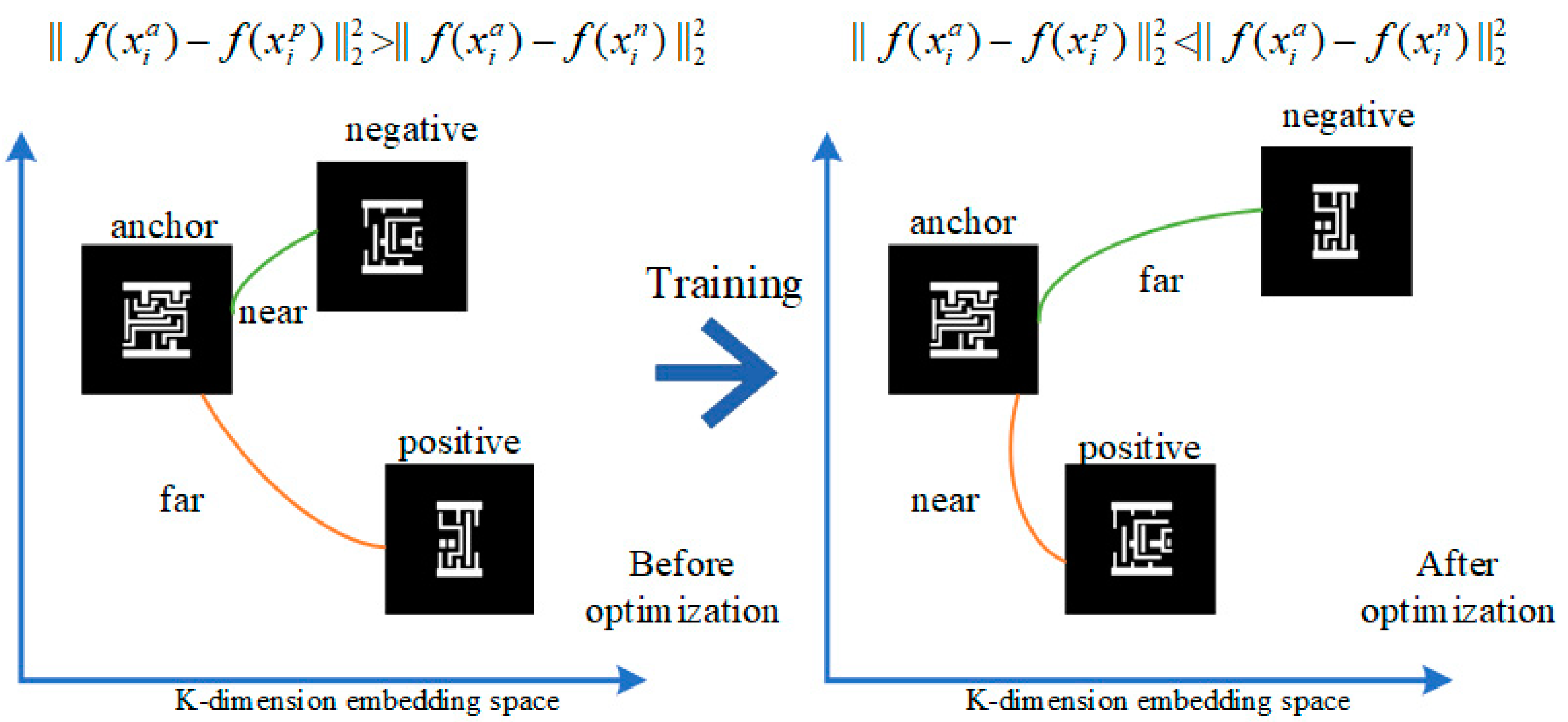
To optimize the CNN model, triplet loss was introduced as the loss function during the training process. This loss ensured that $x_i^a$ (anchor) of a triplet was closer to $x_i^p$ (positive) than to $x_i^n$ (negative). The designed optimization goal of triplet loss is to make embeddings satisfy the inequality shown in Figure 4. This can also be written as follows:

$$\left|\right|f(x_i^a)-f(x_i^p)|{|}_2^2+\alpha <||f(x_i^a)-f(x_i^n)|{|}_2^2,\forall (x_i^a,x_i^p,x_i^n)\in T$$

(2)

where α is the margin that is enforced between positive and negative pairs, T represents all possible triplets for pattern training datasets, and i is the triplet index. The triplet loss in Equation (3) evolves from the inequality above.

$$L={{\displaystyle \sum _i^N\left[\left|\right|f\left(x_i^a\right)-f\left(x_i^p\right)|{|}_2^2-||f\left(x_i^a\right)-f\left(x_i^n\right)|{|}_2^2+\alpha \right]}}_{+}$$

(3)

The loss function uses the Euclidean distance to express the distance between different embeddings. This also implies low within-cluster scatter (WCS) and high between-cluster scatter (BCS), which are the ideal results for the pattern cluster task. Only a portion of all triplets satisfied Equation (2) for the model with the initial parameters. While minimizing the triplet loss, the distance between the anchor and positive decreased, whereas the distance between the anchor and negative increased. Another problem that was addressed was the triplet selection strategy for triplet generators. Theoretically, an anchor sample has many positive and negative matches. If every iteration triplet is generated randomly, many triplets satisfy Equation (2) and do not contribute to the optimization, which means that the loss of these triplets is zero. To avoid this problem, the hard-triplet update strategy was applied, which means that for each anchor, only the closest negative and farthest positive samples were selected to build the “hardest” triplet instead of the “easy” triplet. Every few epochs, the triplet set was updated using the hardest triplet. The optimization algorithm used in the training stage was stochastic gradient descent (SGD), whose update formula is

$$W_{t+1}^l(i)=W_t^l(i)-\eta \cdot \frac{\partial L}{\partial W_t^l(i)}$$

(4)

where $W_t^l(i)$ is the $l$th element in the lth layer of the weight matrix, $t$ is the iteration index, and η is the learning rate. The algorithm allows the model weights in each layer to be updated to minimize the triplet loss.

2.4. DBSCAN Cluster Algorithm

The trained model mapped the image to the embeddings in the feature space. Unlike in the training stage, the model application did not require a feed picture in the form of a triplet. When pattern images were input, the respective embeddings were obtained after the data propagated forward in the model. A clustering algorithm can group these embeddings in a K-dimensional space. Every embedding in the form of a vector in the feature space is a point, and these points have a certain distance apart. The distance is the difference in the results for the SMO content. Based on this idea, DBSCAN was used as the clustering algorithm. Unlike other traditional clustering algorithms, such as the k-means, it does not require the number of clusters but the margin ε, which also appears in the triplet loss formula.

There are several definitions of our DBSCAN algorithm. The relationship between the outliers and core points is shown in Figure 5.

(1)

An embedding point is a core point if at least minPts (set manually) points (including itself) are within a distance ε apart.

(2)

An embedding point is reachable from a core point, if it is within a distance ε from the core point. If embedding B is reachable to embedding A and embedding C is reachable to embedding B, then embedding C is reachable to embedding A.

(3)

Embedding points that are not reachable from any other point are outliers.

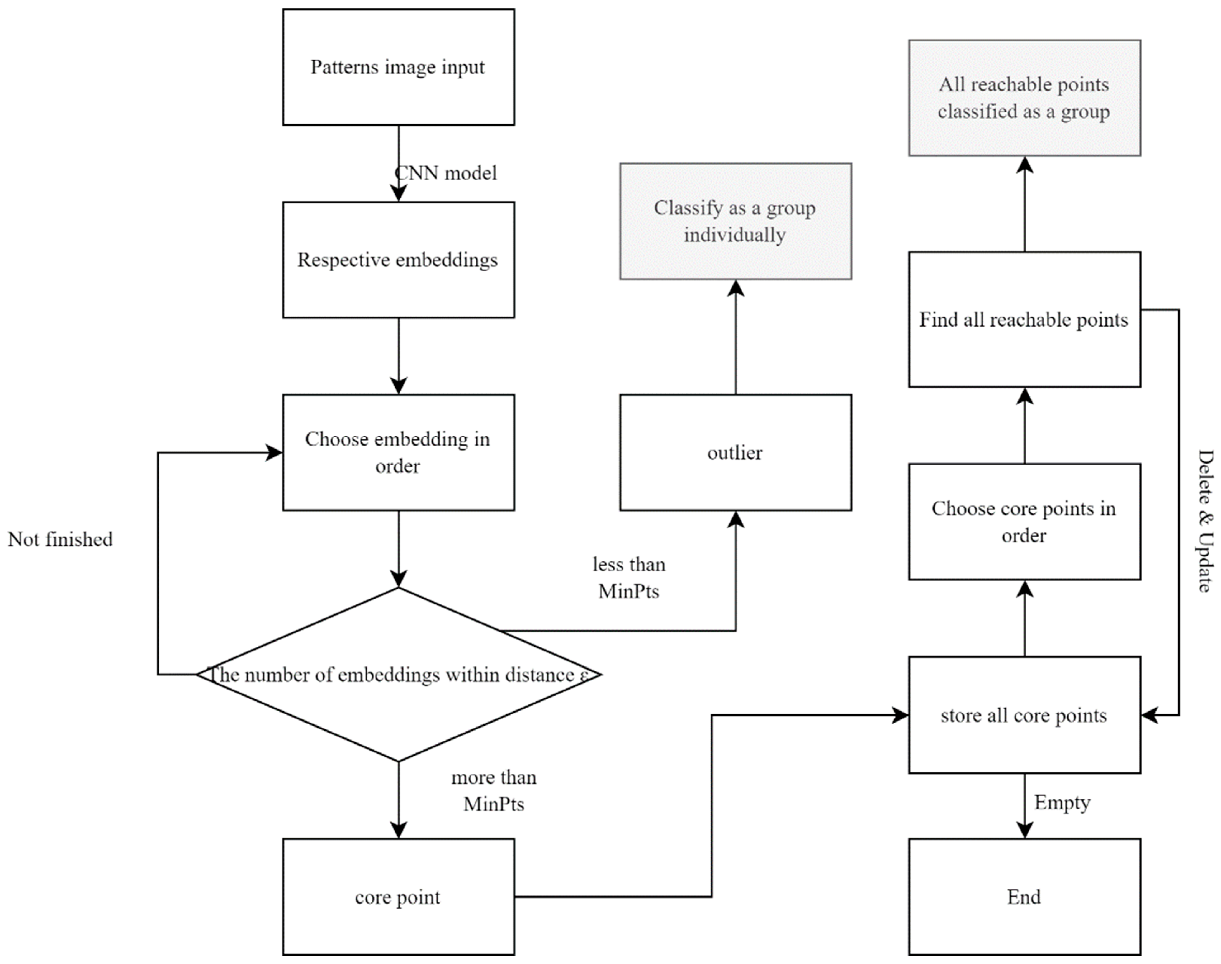
The detailed workflow is shown in Figure 6. The set of pattern embeddings was stored and clustered after the pattern images were mapped onto the feature space. An embedding point can be individually classified as a core point or an outlier until all points are checked, mentioned in Figure 6. All core points were stored, and the outliers were classified into a single group. Considering the pattern selection situation, ε is a margin of $\alpha$ in triplet loss. For each core point, the reachable points were determined individually. Once mutually reachable, they were classified into the same group and deleted from the core point set. If no members remained in the set, the algorithm was terminated. Subsequently, every group had a centroid in the K-dimensional space, and the critical pattern in each cluster could be determined by Equation (5).

$$x_c=\underset{x_i}{\arg \min }||f(x_i)-\frac{1}{N}{\displaystyle \sum _{j=1}^{N}f(x_j)|{|}_2^2}, i,j\in Cluste{r}_{nth}$$

(5)

where $x_c$ is the selected critical pattern, i,j is the index in the nth cluster, N is the number of members in the cluster, and $f(x)$ is the embedding output of the CNN model. The closer the embedding point is to the center, the more representative it is of the cluster. In other words, the pattern embedded nearest to the center of the cluster is the critical pattern.

2.5. Overall Workflow of the Method

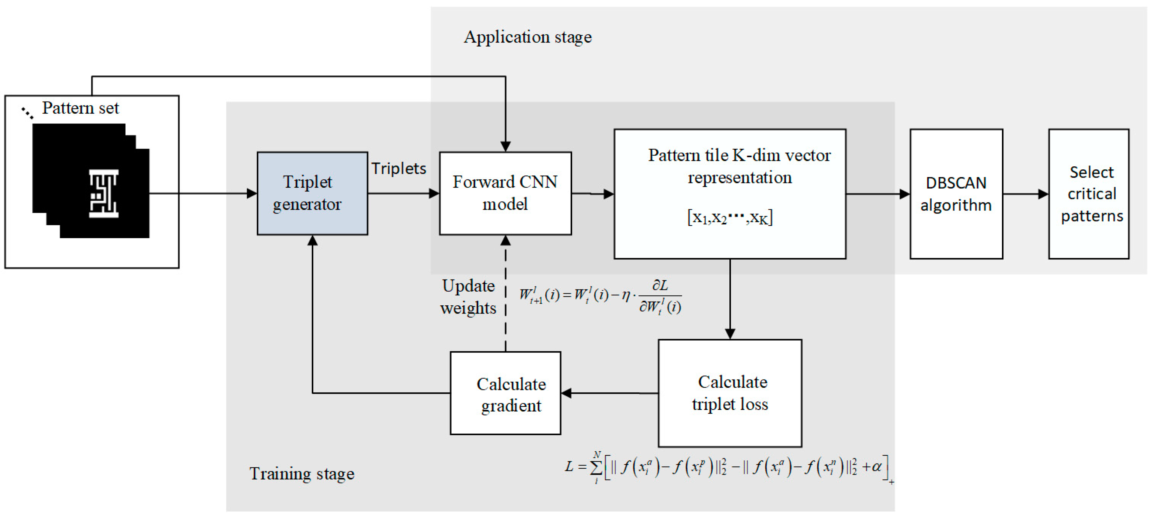
The pattern selection workflow was composed of several substeps after cutting patterns from the full-chip area: pattern transformation, pattern clustering, and critical member selection. This study introduced a CNN in the pattern transformation part and output the CNN embedding to cluster and select critical patterns in later processes. A CNN with updatable parameters can perform nonlinear mapping; thus, it can be trained to obtain the most appropriate mapping relationship from pattern graphics into the abstract space in SMO. The workflow of the proposed critical pattern selection process shown in Figure 7 can be divided into two stages: training and application. Before patterns were fed into the CNN model in the training stage, triplets were generated first through the strategy mentioned in Section 2.3. Then, respective embeddings and their losses after forwarding CNN could be calculated. With the triplet loss, the model could be updated by SGD. The trained model could be applied to achieve the transformation from pattern images to embedding vectors. The DBSCAN algorithm clustered the embeddings and determined the critical members in each cluster based on the distribution of embeddings.

3. Simulation Experiment and Discussion

To demonstrate the advantage of triplet loss, the performances of the untrained and final models were compared from the perspective of the visualized embedding distribution. In addition, the manner in which the value of the loss changed when the number of iterations increased with two different triplet selection strategies and different embedding dimensions was demonstrated. Finally, compared with the pattern selection results of the diffraction signature method, the proposed method simulated a real case using the test data.

3.1. Model Training

The model was pre-trained through the traditional cross-entropy loss in 100 epochs, followed by the triplet loss in 500 epochs, instead of using the direct triplet loss. The pretraining stage helps the formal training stage converge more quickly. The learning rate η in Equation (4) is ${10}^{-4}$ for the pre-training stage and ${10}^{-5}$ for the formal training stage. The optimization process in the formal stage with different triplet selection strategies is shown in Figure 8. In Figure 8a, the hard triplet selection curves converged much more quickly, and their loss could drop to a lower position compared to the random-selection curve. This proves that the hard triplet selection strategy improved optimization performance. As shown in Figure 8b, for different K values, the trends of all three curves were similar, and they all converged in approximately 300 epochs. The final triplet loss was close to zero, implying that the model converged well in the dataset.

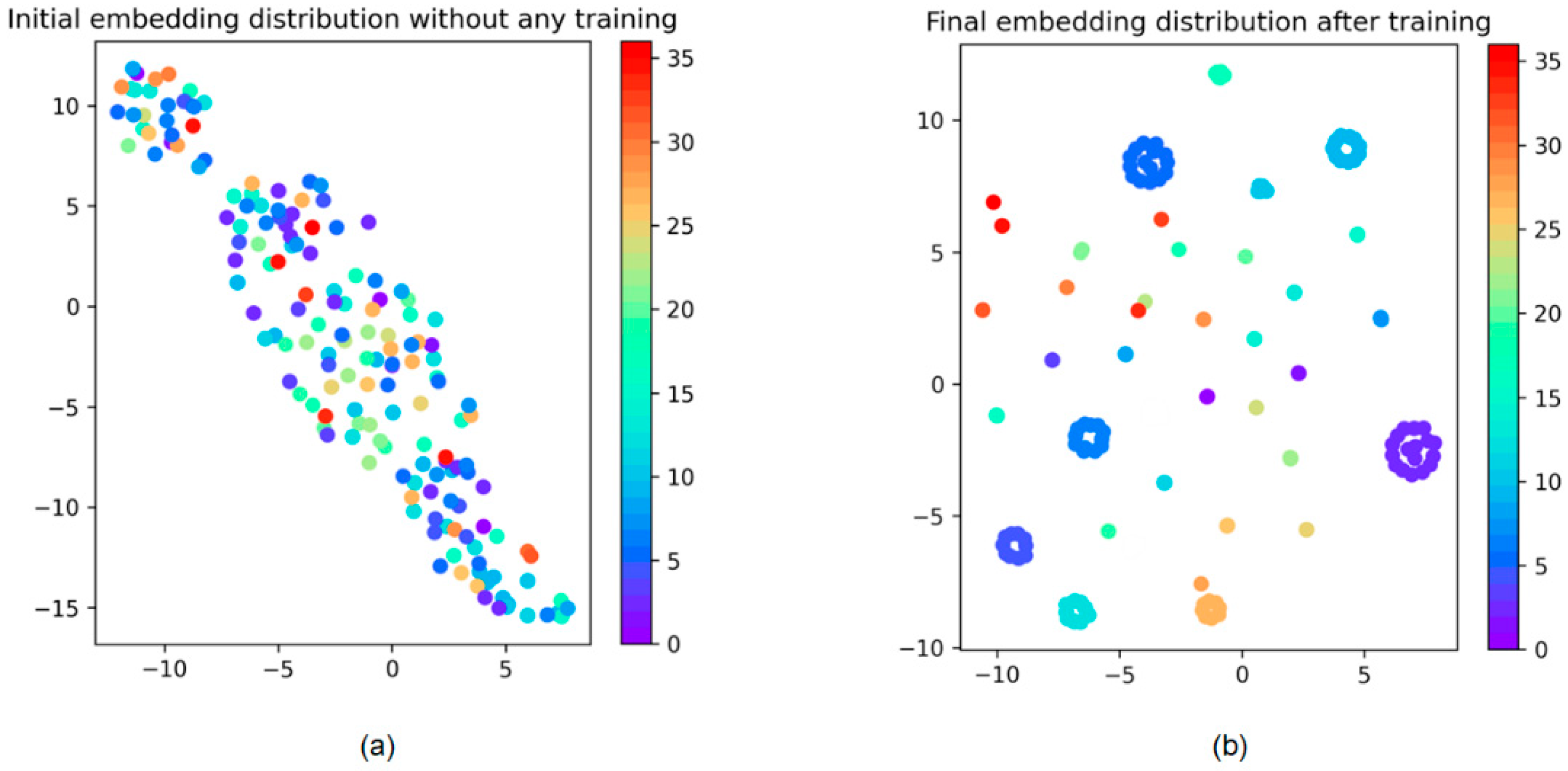
Figure 9 shows the changes in the distribution embedding output from the initial to the final model. The point in the coordinates is embedded from the CNN, and the different colors indicate its group. Because high-dimensional information is difficult to visualize, methods such as principal component analysis (PCA), a dimension reduction method, were applied for visualization. The distribution after projection does not show the exact situation and only contains general information. In Figure 8a, the embedding distribution was chaotic, and patterns from different clusters mixed without any rules. The distribution after optimizing the model was much better, as shown in Figure 9b. Almost all patterns belonging to the same group were held together, and different groups had margins between each other, even though some points did not obey these rules. This indicates a small in-group distance and a large between-group distance.

The selection of embedding dimensions is also discussed. The embedding dimensions must satisfy the complexity of the problem. Considering the black-and-white mask image, the embedding dimension should not be large. To test the dimension value K’s impact, experiments were performed with different K values. The validation rates and final losses for K = 32, 64, and 128 are shown in

Table 1. Validation rate and average loss with different embedding dimensions (K).

Embedding Dimension	32	64	128
VAL (%)	96.42	97.62	95.83
Average Loss	0.012	0.009	0.018

. The validation rate is defined as follows:

$$VAL=\frac{TA}{P_{same}}$$

(6)

where $P_{same}$ is the number of all pattern pairs $(x_i,x_j)$ in the same group. $TA$ denotes true accept, which means pairs that are correctly classified as the same.

The final validation rate and average loss were similar for different embedding dimensions. The best performance was obtained at K = 64. When the number of embedding dimensions was increased to 128, the performance of the model worsened. However, the difference was small for different K values used in the experiment. To decrease the computation and storage costs, K = 32 is a better choice.

3.2. Pattern Cluster and Selection in Test Data

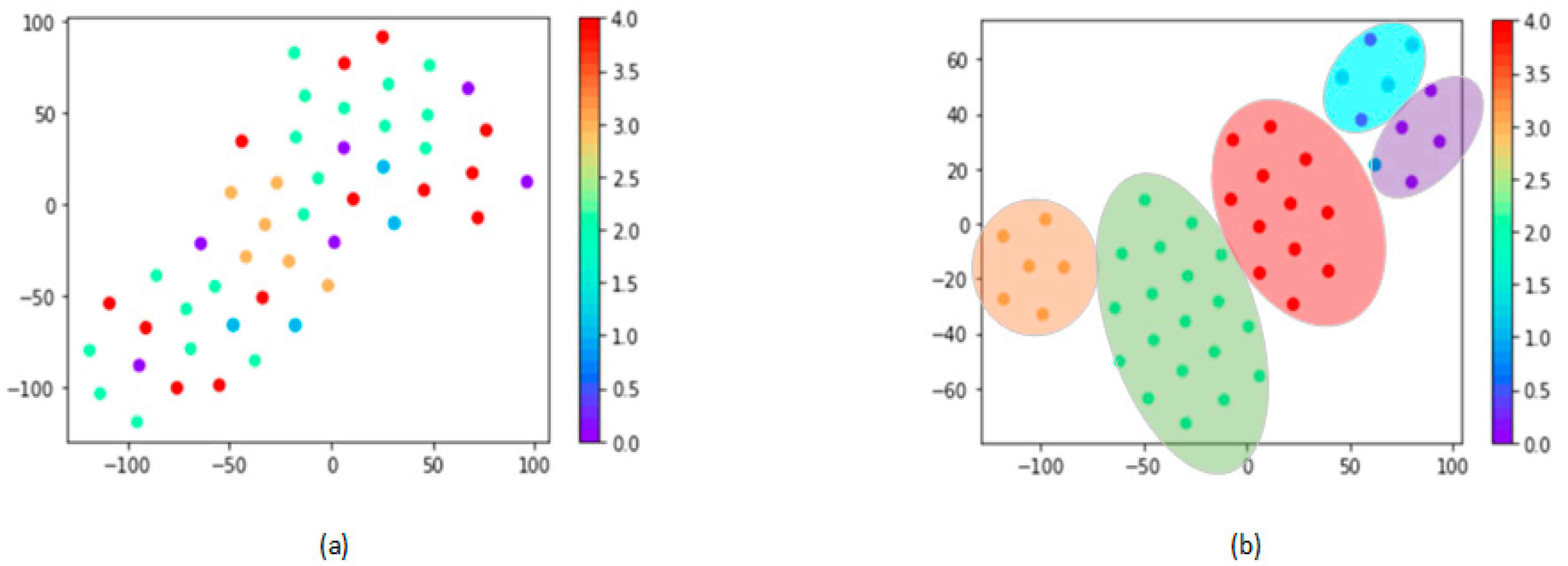
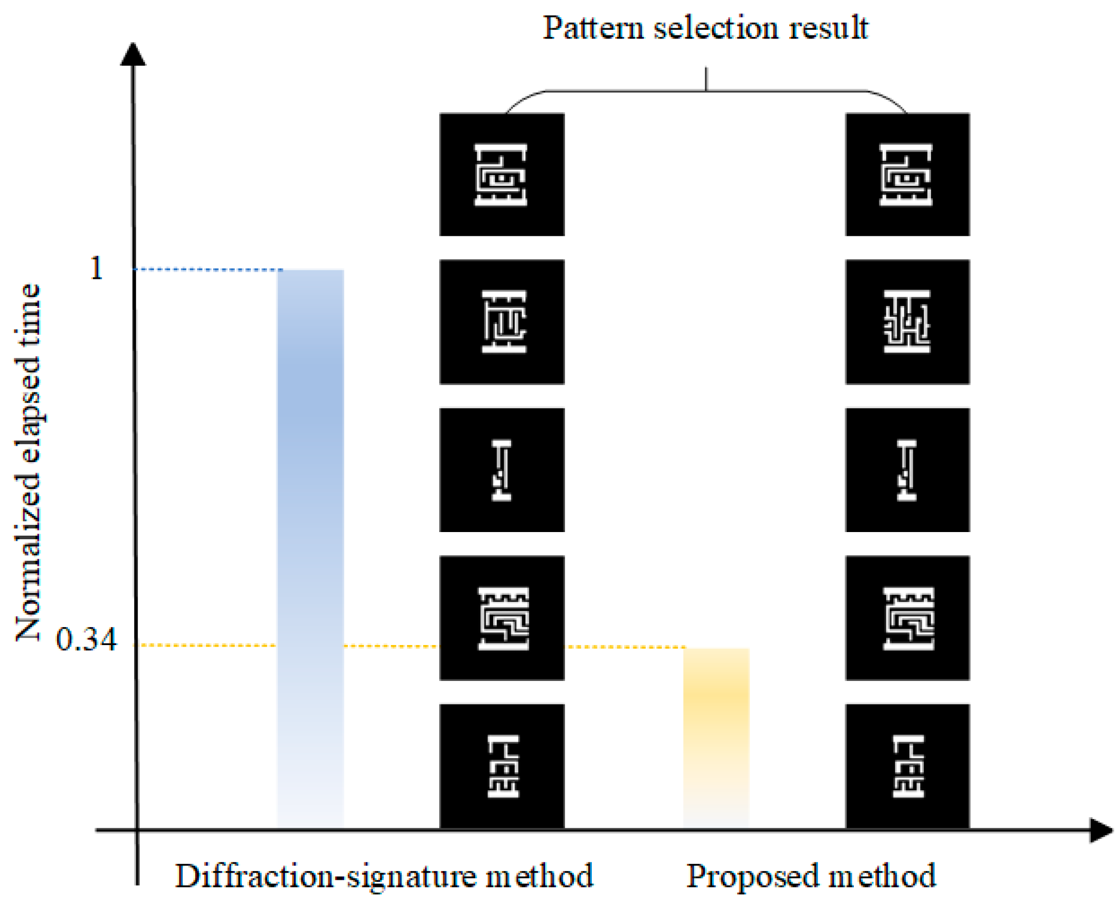
This section discusses the test data used in the simulation to reveal the pattern cluster and critical pattern selection results. The workflow of the model was illustrated in Figure 2. The test data were fed into the CNN model and transferred to the embeddings in the K-dimensional space. Figure 10 shows the distribution of the test data using the PCA algorithm before and after training. The distribution of the embedding of the test data changed from disordered to ordered, which proves the robustness and generalization ability of our model. Additionally, after applying the DBSCAN method, the final cluster result was obtained, as shown in Figure 10. Each circle represents a cluster. The centroid of each cluster can be determined, and the embedding closest to the centroid is the critical pattern. A comparison of the selection results of the proposed method and ASML’s is presented in Figure 11. Compared with the diffraction signature method—the leading one—only one selected critical pattern was different. The other critical patterns were identical. It shows that the CNN model learned the diffraction signature knowledge successfully and had good robustness.

The diffraction signature method takes considerable time in a real case because the algorithm has to extract every member’s diffraction signature and compare it with those of other members. Because the method, a CNN paradigm, can be parallelized easily on the GPU platform, which accelerates the computation process, in the proposed algorithm, although the model training required a few hours, forward propagation in the model application and clustering required only a third of the time compared with that of the diffraction signature method from Figure 11. Thus, the computational cost of the model application was much lower when the number of patterns was large compared with that of the diffraction signature method. This is another advantage of the proposed method.

4. Conclusions

This study proposes a critical pattern selection method based on the cluster selection architecture. This method mapped two-dimensional pattern image data to k-dimensional embeddings in the feature space, which were then clustered via the DBSCAN algorithm, thus leveraging the distribution of the embeddings. The mapping function was achieved through the VGG convolutional neural network (CNN). The core idea of the optimization process is the triplet loss, which cooperated with the back-propagation algorithm to decrease the Euclidean distance between patterns from the same group and increase the Euclidean distance between patterns from different groups. Moreover, the architecture within the proposed method can be updated and further enhanced using multiple labeled datasets in the future without increasing the computational cost of model application. Simulation results revealed the success of the CNN model in accomplishing pattern clustering and selection tasks. The visualized results of the embedding distribution showed that they absolutely conformed to low within-class scatter (WCS) and high between-class scatter (BCS) situations in the K-dimension feature space. The proposed method maintains high clustering and selection accuracy with low computation cost and has a major advantage of not requiring manual configuration of the cluster number.

References

1. Liu, A.C.; Lin, B.J. A study of projected optical images for typical IC mask patterns illuminated by partially coherent light. IEEE Trans. Electron Devices 1983, 30, 1251–1263. [Google Scholar] [CrossRef]
2. Wong, A.K.-K. Resolution Enhancement Techniques in Optical Lithography; SPIE: Bellingham, WA, USA, 2001. [Google Scholar]
3. Melville, D.O.S.; Rosenbluth, A.E.; Waechter, A.; Millstone, M.; Tirapu-Azpiroz, J.; Tian, K.; Lai, K.; Inoue, T.; Sakamoto, M.; Adam, K.; et al. Computational lithography: Exhausting the resolution limits of 193-nm projection lithography systems. J. Vac. Sci. Technol. B 2011, 29, 06FH04. [Google Scholar] [CrossRef]
4. Abrams, D.S.; Pang, L. Fast inverse lithography technology. In Optical Microlithography XIX, Proceedings of the SPIE 31st International Symposium on Advanced Lithography, San Jose, CA, USA, 19–24 February 2006; SPIE: Bellingham, WA, USA, 2006; Volume 6154, pp. 534–542. [Google Scholar]
5. Ma, X.; Arce, G.R. Computational Lithography; Wiley Series in Pure and Applied Optics; Wiley: London, UK, 2010. [Google Scholar]
6. Rosenbluth, A.E.; Melville, D.O.; Tian, K.; Bagheri, S.; Tirapu-Azpiroz, J.; Lai, K.; Waechter, A.; Inoue, T.; Ladanyi, L.; Barahona, F.; et al. Intensive optimization of masks and sources for 22 nm lithography. Proc. SPIE 2009, 7274, 727409. [Google Scholar]
7. Rosenbluth, A.E.; Bukofsky, S.J.; Hibbs, M.S.; Lai, K.; Molless, A.F.; Singh, R.N.; Wong, A. Optimum mask and source patterns to print a given shape. Proc. SPIE 2001, 4346, 486–502. [Google Scholar]
8. Ma, X.; Arce, G.R. Pixel-based simultaneous source and mask optimization for resolution enhancement in optical lithography. Opt. Express 2009, 17, 5783–5793. [Google Scholar] [CrossRef]
9. Peng, Y.; Zhang, J.; Wang, Y.; Yu, Z. Gradient-based source and mask optimization in optical lithography. IEEE Trans. Image Process. 2011, 20, 2856–2864. [Google Scholar] [CrossRef]
10. Ma, X.; Han, C.; Li, Y.; Dong, L.; Arce, G.R. Pixelated source and mask optimization for immersion lithography. J. Opt. Soc. Am. A 2013, 30, 112–123. [Google Scholar] [CrossRef]
11. Jia, N.; Lam, E.Y. Pixelated source mask optimization for process robustness in optical lithography. Opt. Express 2011, 19, 19384–19398. [Google Scholar] [CrossRef]
12. Li, J.; Lam, E.Y. Robust source and mask optimization compensating for mask topography effects in computational lithography. Opt. Express 2014, 22, 9471–9485. [Google Scholar] [CrossRef]
13. Peng, F.; Shen, Y. Source and mask co-optimization based on depth learning methods. In Proceedings of the 2018 China Semiconductor Technology International Conference (CSTIC), Shanghai, China, 11–12 March 2018; pp. 1–3. [Google Scholar]
14. Shen, Y. Lithographic source and mask optimization with narrow-band level-set method. Opt. Express 2018, 26, 10065–10078. [Google Scholar] [CrossRef]
15. Fühner, T.; Erdmann, A. Improved mask and source representations for automatic optimization of lithographic process conditions using a genetic algorithm. Proc. SPIE 2005, 5754, 41. [Google Scholar]
16. Yang, C.; Li, S.; Wang, X. Efficient source mask optimization using multipole source representation. J. Micro/Nanolith. 2014, 13, 043001. [Google Scholar] [CrossRef]
17. Wang, L.; Li, S.; Wang, X.; Yang, C. Source mask projector optimization method of lithography tools based on particle swarm optimization algorithm. Acta Opt. Sin. 2017, 37, 1022001. [Google Scholar] [CrossRef]
18. Tsa, M.-C.; Hsu, S.; Chen, L.; Lu, Y.-W.; Li, J.; Chen, F.; Chen, H.; Tao, J.; Chen, B.-D.; Feng, H.; et al. Full-chip source and mask optimization. Proc. SPIE 2011, 7973, 79730A. [Google Scholar]
19. DeMaris, D.L.; Gabrani, M.; Volkova, E. Method of Optimization of a Manufacturing Process of an Integrated Layout. U.S. Patent US8667427, 4 March 2014. [Google Scholar]
20. Lai, K.; Gabrani, M.; Demaris, D.; Casati, N.; Torres, A.; Sarkar, S.; Strenski, P.; Bagheri, S.; Scarpazza, D.; Rosenbluth, A.E.; et al. Design specific joint optimization of masks and sources on a very large scale. Proc. SPIE 2011, 7973, 797308. [Google Scholar]
21. Zhang, D.; Chua, G.; Foong, Y.; Zou, Y.; Hsu, S.; Baron, S.; Feng, M.; Liu, H.-Y.; Li, Z.; Schramm, J.; et al. Source mask optimization methodology (SMO) and application to real full chip optical proximity correction. Proc. SPIE 2012, 8326, 83261V. [Google Scholar]
22. Liao, L.; Li, S.; Wang, X.; Zhang, L.; Gao, P.; Wei, Y.; Shi, W. Critical pattern selection method for full-chip source and mask optimization. Opt. Express 2020, 28, 20748–20763. [Google Scholar] [CrossRef]
23. Krizhevsky, A.; Sutskever, I.; Hinton, G.E. ImageNet classification with deep convolutional neural networks. In Proceedings of the International Conference on Neural Information Processing Systems, Lake Tahoe, NV, USA, 3–6 December 2012; pp. 1097–1105. [Google Scholar]
24. Simonyan, K.; Zisserman, A. Very Deep Convolutional Networks for Large-Scale Image Recognition. In Proceedings of the International Conference on Learning Representations, San Diego, CA, USA, 7–9 May 2015. [Google Scholar]
25. Szegedy, C.; Liu, W.; Jia, Y.; Sermanet, P.; Reed, S.; Anguelov, D.; Erhan, D.; Vanhoucke, V.; Rabinovich, A. Going deeper with convolutions. In Proceedings of the IEEE Conference on Computer Vision and Pattern Recognition, Boston, MA, USA, 7–12 June 2015. [Google Scholar]
26. He, K.; Zhang, X.; Ren, S.; Sun, J. Identity Mappings in Deep Residual Networks. In Proceedings of the European Conference on Computer Vision, Amsterdam, The Netherlands, 11–14 October 2016; pp. 630–645. [Google Scholar]
27. He, K.; Zhang, X.; Ren, S.; Sun, J. Deep residual learning for image recognition. In Proceedings of the IEEE Conference on Computer Vision and Pattern Recognition (CVPR), Las Vegas, NV, USA, 27–30 June 2016. [Google Scholar]
28. Zhang, J.; Ma, X.; Zhang, S.; Zheng, X. Lithography layout classification based on graph convolution network. Proc. SPIE Opt. Microlithogr. 2021, 11613, 116130U. [Google Scholar]
29. Alwattar, T.; Mian, A. Development of an Elastic Material Model for BCC Lattice Cell Structures Using Finite Element Analysis and Neural Networks Approaches. J. Compos. Sci. 2019, 3, 33. [Google Scholar] [CrossRef]
30. Alwattar, T.A.; Mian, A. Developing an Equivalent Solid Material Model for BCC Lattice Cell Structures Involving Vertical and Horizontal Struts. J. Compos. Sci. 2020, 4, 74. [Google Scholar] [CrossRef]
31. Schroff, F.; Kalenichenko, D.; Phillbin, J. FaceNet: A unified embedding for face recognition and clustering. In Proceedings of the IEEE Conference on Computer Vision and Pattern Recognition (CVPR), Boston, MA, USA, 7–12 June 2015. [Google Scholar]
32. Ester, M.; Kriegel, H.-P.; Sander, J.; Xu, X. A Density-based Algorithm for Discovering Clusters in Large Spatial Databases with Noise; AAAI Press: Washington, DC, USA, 1996. [Google Scholar]
33. Wong, K.K. Optical Imaging in Projection Microlithography; SPIE Press: Bellingham, WA, USA, 2005. [Google Scholar]
34. Silvaco Inc. PDK 45 nm Open Cell Library. Available online: https://eda.ncsu.edu/freepdk/freepdk45 (accessed on 1 November 2022).
35. Socha, R. Freeform and SMO. Proc. SPIE 2011, 7973, 797305. [Google Scholar]
Figure 1. Schematic of the lithography optical system.
Photonics 10 01186 g001
Figure 2. Diagram for determining whether two patterns belong to same group in labelling dataset.
Photonics 10 01186 g002
Figure 3. Structure of VGG-16.
Photonics 10 01186 g003
Figure 4. The optimization process by triplet loss.
Photonics 10 01186 g004
Figure 5. Diagram of the relationships of elements in the DBSCAN algorithm (minPts = 3, A and other red points are core points because the surrounding area in a radius of ε has more than minPts. They are reachable to each other and form a cluster. Embeddings B and C are not core points, but they are reachable from red points, thus belonging to the cluster as well. Point N has no neighbor points; therefore, it is an outlier).
Photonics 10 01186 g005
Figure 6. Flowchart of the DBSCAN algorithm.
Photonics 10 01186 g006
Figure 7. Workflow of the whole critical pattern selection process.
Photonics 10 01186 g007
Figure 8. Triplet loss convergence curves for different (a) triplet selection strategies and (b) embedding dimensions.
Photonics 10 01186 g008
Figure 9. Embedding distribution of the training data (a) without training and (b) after training in 500 epochs. The X- and Y-axis are the two projected axes after PCA.
Photonics 10 01186 g009
Figure 10. Test data’s embedding distribution visualized by PCA (a) without training and (b) after training in 500 epochs.
Photonics 10 01186 g010
Figure 11. Critical pattern selection results and eclipsed time from a test set achieved through the ASML’s and proposed methods.
Photonics 10 01186 g011