Temperature Demodulation for an Interferometric Fiber-Optic Sensor Based on Artificial Bee Colony–Long Short-Term Memory

Abstract

Demodulation methods play a critical role in achieving high-performance interferometric fiber-optic temperature sensors. However, the conventional passive 3 × 3 coupler demodulation method overlooks certain issues, such as the non-1:1:1 splitting ratio of the coupler, resulting in a non-ideal phase difference in the three output interference signals. These problems significantly impact the measurement results of interferometric temperature sensors. In this paper, we propose a novel arc-tangent method based on a 3 × 3 coupler and a demodulation algorithm combining long short-term memory (LSTM) with an artificial bee colony (ABC). The arc-tangent method is employed to enhance the input phase signal of the ABC-LSTM network model and establish a nonlinear mapping between the phase signal and temperature, effectively preventing the influence of the spectral ratio and phase difference of the 3 × 3 coupler on temperature demodulation. The proposed ABC-LSTM method achieves high-resolution measurements with an interval of 0.10 °C, and the absolute error is below 0.0040 °C within the temperature range of 25.00–25.50 °C. To demonstrate the stability and adaptability of the proposed method under long-term constant temperature conditions, we conducted measurements for approximately three hours in a controlled temperature environment set at 25.00 °C. Experimental results indicate that the maximum error of LSTM-ABC method remains around 0.0040 °C, outperforming the conventional algorithm (0.0095 °C). Furthermore, when comparing the average error values of the conventional passive 3 × 3 coupler method (0.0023 °C), LSTM model (0.0019 °C), and ABC-LSTM model (0.0014 °C), it is evident that the demodulation results of the ABC-LSTM method exhibit the highest level of stability. Therefore, the ABC-LSTM method enhances the accuracy and reliability of interferometric fiber-optic temperature-sensing systems.

1. Introduction

Interferometric fiber-optic temperature sensors have the advantages of a light weight, small volume, high sensitivity, and a multiplexing system that easily forms distributed measurements. It is widely used in fields such as aerospace, geological exploration, and object detection in the marine environment [1,2,3]. In an interferometric sensor, the measured temperature is encoded in an interference signal phase. Therefore, phase demodulation is critical in interferometry, as its demodulation accuracy directly affects the performance of the interferometric temperature sensor.

Conventional passive 3 × 3 coupler demodulation (e.g., NPS method) is considered the most practical method due to its properties of a large dynamic range and high sensitivity and linearity [4]. However, it must overcome the problem of the 3 × 3 fiber-optic coupler with an unequal splitting ratio, which causes an intrinsic phase difference between any pair of return ports so they cannot be equal to 120° [5]. Y. Pang et al. used the peak-to-peak detection method to remove the DC component and compensate for the AC component coefficient of the three interference signals [6]. This method prevents the problem of an inconsistent coupler splitting ratio. However, when the demodulation phase is less than π, the extreme value of the DC offset may not be accurately measured. Fan P et al. introduced an elliptic fitting algorithm (EFA) into phase demodulation to address problems with DC component deviation, imbalance, and phase differences exhibited by interference signals [7]. However, the accuracy of the elliptical fitting method declines for phase signals near zero or below π/2. Moreover, this approach is exclusively suitable for dynamical temperature demodulation and cannot be applied to static temperature measurement. This is because interference signals obtained in a static environment include a constant phase value, making elliptical fitting impractical since any two interferometric signals would only form many repeating points.

Deep learning is a machine learning technology composed of multilayer nonlinear operating units which has been developed rapidly in recent years and is widely used in the optical field. Feng et al. demonstrated that phase demodulation accuracy can be improved using a convolutional neural network (CNN). By quickly estimating the numerator and denominator of the arc-tangent function with CNN, high-precision, edge-preserving phase reconstruction can be achieved [8]. Sun et al. applied CNN to high-precision ultra-fast phase demodulation from the measurement of optical surfaces, achieving an RMS accuracy of 0.01 λ [9]. However, it should be noted that this method is more suitable for image processing. For a one-dimensional interference signal, it needs to be converted into a two-dimensional image to achieve temperature demodulation, so the whole process is complicated.

As one of the classical deep learning models, long short-term memory (LSTM) has a strong feature extraction capability and powerful nonlinear mapping capability. It is capable of efficiently extracting critical measurement features from one-dimensional signals, making LSTM highly promising for signal demodulation [10]. Moreover, by using the feedback mechanism during the LSTM network training process, the nonlinear correlation between phase signals and temperature can be continuously corrected until the error of the demodulation result is minimized. The constructed network model eliminates the influence of inconsistent splitting ratios and phase differences between adjacent signals that are not 120°. However, random initialization of weights and thresholds in LSTM networks can lead to slower convergence and the risk of becoming trapped in local minima [11]. To achieve efficient global optimization, the artificial bee colony (ABC) algorithm uses the optimal and historically optimal locations of employed bees in the population [12]. This feature can be used to optimize the weights and threshold parameters of the LSTM network, thus preventing local optimization within the solvable space. Inspired by this, this paper proposes a demodulation technique using ABC-LSTM. The model is trained to learn the correlation between temperature and phase signals from the 3 × 3 coupler. Experimental results demonstrate that the proposed algorithm outperforms the conventional passive 3 × 3 coupler phase demodulation.

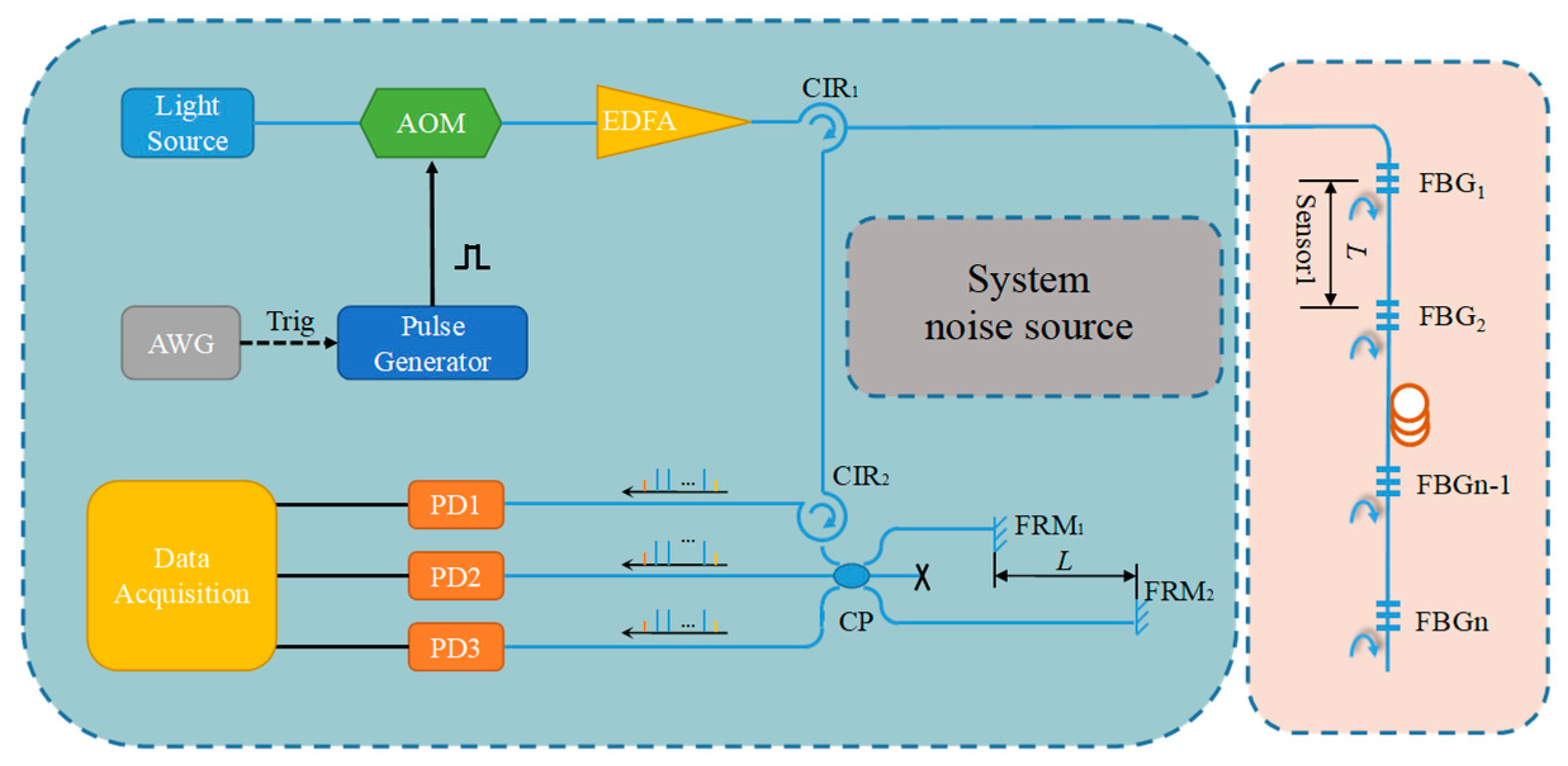
2. F-P Interferometric Fiber-Optic Temperature Sensor Array

The structure of the FBG-FP interferometric temperature-sensing system is shown in Figure 1. A continuous laser beam with a central wavelength of 1550 nm is modulated by an acousto-optic modulator (AOM), resulting in a series of light pulses. After amplifying the modulated light using a fixed-gain erbium-doped fiber amplifier (EDFA), the resulting light pulses are introduced into the FBG-FP sensor in a temperature-controlled environment. In the sensor array, two adjacent FBGs with an optical fiber connecting them comprise a sensor unit. The light pulse reflected by each FBG is directed through circulator1(CIR1) and circulator2(CIR2) into an unbalanced Michelson interferometer, where interference fringes are observed at a 3 × 3 coupler. The resulting optical interference signals are detected using three photodetectors (PDs), and the corresponding electrical signals are acquired using a data acquisition card and transmitted to a computer for real-time analysis and display.

The three interference signals of the 3 × 3 coupler under ideal conditions can be expressed as

$$I_k=A+B\cos (\phi (t)-\frac{2\pi }{3}(k-1)),k=1,2,3$$

(1)

where A is the average light power of the detected signals, B is the amplitude of the interference signal, and $\phi \left(t\right)$ is the phase change caused by temperature.

The conventional NPS demodulation algorithm requires the three interfering signals to be added to obtain the direct current (DC) signal. Subsequently, the DC component is subtracted from these signals. This process can be expressed as

$$\frac{I_1(t)+I_2(t)+I_3(t)}{3}=A$$

(2)

$${I^{\prime }}_k=B\cos (\phi (t)-\frac{2\pi }{3}(k-1)),k=1,2,3$$

(3)

The three signals in Equation (3) are subjected to a sequence of differential, integral, and derivative operations to obtain the $\phi \left(t\right)$, which can be expressed as [13]

$$\phi (t)=\frac{{\displaystyle {\int }_0^t(I_1^{\prime }(\frac{d{I}_2^{\prime }}{dt}-\frac{d{I}_3^{\prime }}{dt})+I_2^{\prime }(\frac{d{I}_3^{\prime }}{dt}-\frac{d{I}_1^{\prime }}{dt})+I_3^{\prime }(\frac{d{I}_1^{\prime }}{dt}-\frac{d{I}_2^{\prime }}{dt}))dt}}{\sqrt{3}(I_1^{\prime }{}^2+I_2^{\prime }{}^2+I_3^{\prime }{}^2)}$$

(4)

The temperature sensitivity of the sensor is determined by fitting the demodulated phase signal $\phi \left(t\right)$, and the temperature value is calculated by dividing the phase by the corresponding temperature sensitivity. However, in practical scenarios, the performance of the 3 × 3 coupler is suboptimal, resulting in an inconsistent splitting ratio and non-uniform phase difference. Accordingly, the DC and AC components of the three interference signals in Equation (1) vary, and the phase difference between adjacent signals deviates from 120 degrees, negatively affecting the effectiveness of the demodulation algorithm.

3. F-P Temperature Demodulation Model Based on ABC-LSTM

To solve the above problems, we use the feedback mechanism in the training process of the LSTM network, which can continuously correct the nonlinear relationship between the phase signal and temperature until the demodulation result is in line with the theoretical temperature value. The constructed network model effectively circumvents problems associated with inconsistent splitting ratios and non-120° phase differences between adjacent signals in the demodulation process. The focus of this section is to derive the phase information initially using the arc-tangent algorithm, designate it as the input of the network model, and designate temperature as the output of the network model. Subsequently, the corresponding ABC-LSTM neural network model is developed based on input and output and used to learn the information of phase changes with temperature.

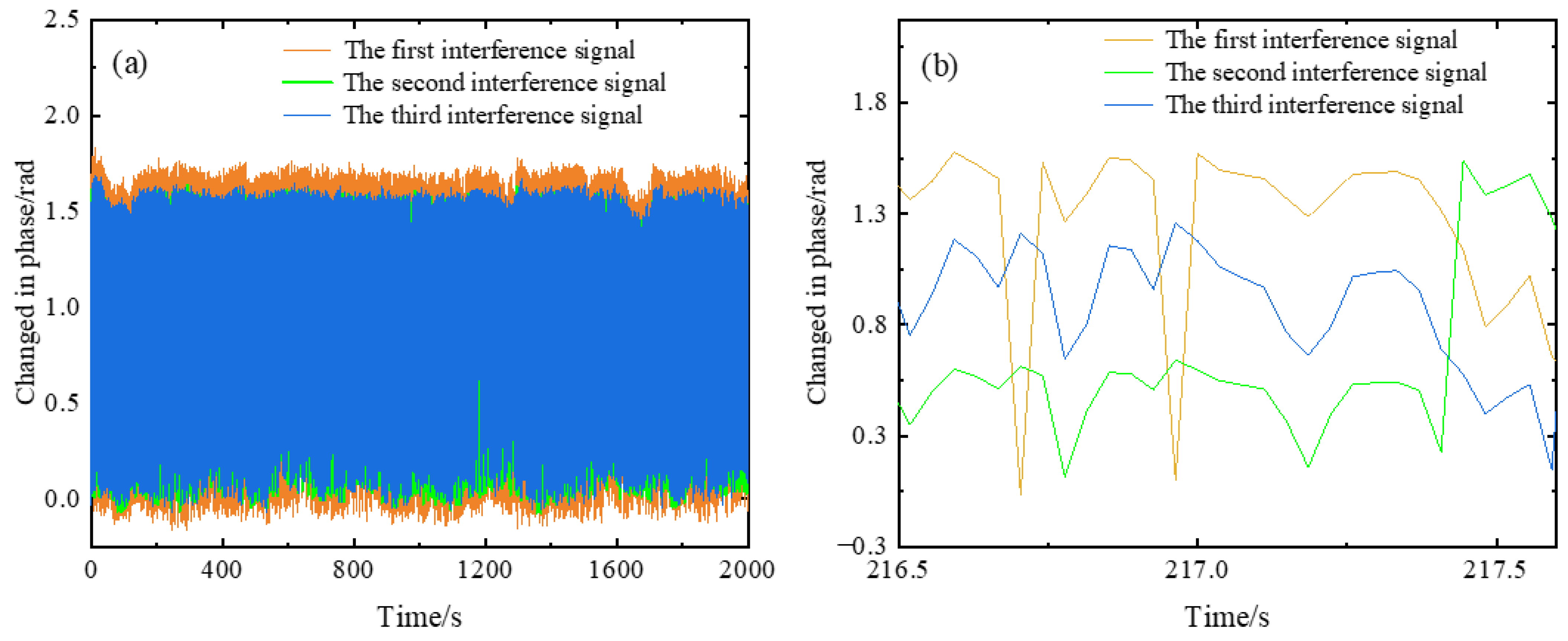
3.1. Modified Arc-Tangent Algorithm Based on 3 × 3 Coupler

From Equation (1), it can be seen that the range of interference signals is limited by the cosine function, which cannot truly reflect the temperature trend. Therefore, it is necessary to demodulate the phase contained in three interference signals to effectively reflect temperature changes. According to Equation (4), conventional demodulation algorithms, which involve differential, integral, derivative, and other operations, can increase noise in the demodulated phase information. Therefore, the results of the conventional algorithm are used as input to the network model, which affects the stability and effectiveness of the demodulation result.

In order to optimize the input of the network model, we propose an arc-tangent algorithm based on a 3 × 3 coupler for demodulating phase information. The three de-DC interference signals in Equation (3) are converted into arc-tangent forms, thus providing a phase signal that reflects temperature information. This process can be expressed as

$${{\phi }^{\prime }}_1(t)=\phi (t)+{\theta }_1=\arctan \frac{\sqrt{3}}{2}(\frac{{I^{\prime }}_1}{{I^{\prime }}_2}+\frac{1}{2})$$

(5)

$${{\phi }^{\prime }}_2(t)=\phi (t)+{\theta }_2=\arctan \frac{\sqrt{3}}{2}(\frac{{I^{\prime }}_2}{{I^{\prime }}_3}+\frac{1}{2})$$

(6)

$${{\phi }^{\prime }}_3(t)=\phi (t)=\arctan \frac{\sqrt{3}}{2}(\frac{{I^{\prime }}_3}{{I^{\prime }}_1}+\frac{1}{2})$$

(7)

where ${\theta }_1$ is caused by the phase difference between the first channel interference signal and the second channel interference signal. ${\theta }_2$ is caused by the phase difference between the second channel interference signal and the third channel interference signal.

The three phase signals, ${\phi }_1^{\prime }\left(t\right)$, ${\phi }_2^{\prime }\left(t\right)$, and ${\phi }_3^{\prime }\left(t\right)$, are unwrapped [14] to obtain reconstructed phase signals, ${\phi }_1^{″}\left(t\right),$ ${\phi }_2^{″}\left(t\right), \mathrm{a}\mathrm{n}\mathrm{d} {\phi }_3^{″}\left(t\right)$, that can reflect temperature information. Compared with the conventional passive 3 × 3 coupler algorithm, the modified arc-tangent algorithm has a simpler calculation process with the added advantage of eliminating noise from differential, integral, and derivative operations. Moreover, the demodulation performance of the multivariate input model exceeds that of the single-variable model [15], whereas the traditional NPS algorithm can only obtain a single signal as input for the ABC-LSMT model. Our proposed modified arc-tangent method extracts three phase signals as input for the ABC-LSMT model. Therefore, using the three-phase signals obtained using the arc-tan algorithm for input into the ABC-LSMT model can more accurately reflect temperature changes.

To demonstrate the results of phase demodulation using the modified arc-tangent algorithm, we conducted simulations using three interferometric signals. To ensure that the parameters of the simulation signals were consistent with the actual situation, we used the ellipse fitting algorithm [16] to fit the measured three interference signals, enabling us to calculate the average light power of the interference signals, the amplitude, and the phase differences between the two interference signals. On calculation, we determined that the average light power of the interference signals was about −0.9~−0.7 V. The amplitude of the interference signals was about −1.9~−1.5 V. The phase difference between the two adjacent signals was roughly 116.2~117.8°. Therefore, we set the interference signals $I_1=-0.80-1.70\cos \phi (t)$, $I_2=-0.83-17.5\cos (\phi (t)+0.65\pi )$, and $I_3=-0.86-1.80\cos (\phi (t)-0.655\pi )$, where the function $\phi \left(t\right)$ consists of five staircases, each connected by a uniform slope of 0.1. The simulation results are shown in Figure 2, wherein the black line is the phase signal ${\phi }_1^{″}\left(t\right)$, the red line is the phase signal ${\phi }_2^{″}\left(t\right)$, the blue line is the phase signal ${\phi }_3^{″}\left(t\right)$, and the green line is the phase signal $\phi \left(t\right)$. It can be seen from Figure 2a that the overall change trend of the three normalized unwrapped phase signals ${\phi }_1^{″}\left(t\right),$ ${\phi }_2^{″}\left(t\right), {\mathrm{a}\mathrm{n}\mathrm{d}\phi }_3^{″}\left(t\right)$ is consistent with that of the original phase signal $\phi \left(t\right)$. The correlation coefficients between the three phase signals and the original phase signal $\phi \left(t\right)$ are all 1. These results indicate that unwrapping phase signals can effectively reflect preset value variations. In addition, from the detailed diagram in Figure 2b, it is evident that the three phase signals exhibit similar upward and downward trends, which is caused by the phase difference between the three signals.

To demonstrate the efficacy of the aforementioned process in practical measurements, we selected the training data in an environment where the temperature was raised from 2.00 °C to 35.00 °C with an interval of 0.10 °C. The three normalized unwrapped phase signals are shown in Figure 3. As shown in Figure 3a, the temperature change information is clearly reflected in the change trend of the three phase signals. In addition, Figure 3b provides a detailed view showing that the change trend of the three normalized unpacked signals is similar, consistent with the simulation results. Calculation of the correlation coefficient revealed high correlations of 0.9924, 0.9890, and 0.9472 between the three phase signals and temperature, respectively. This suggests that unwrapped phase signals can be used as effective inputs for the ABC-LSMT model to accurately reflect temperature changes.

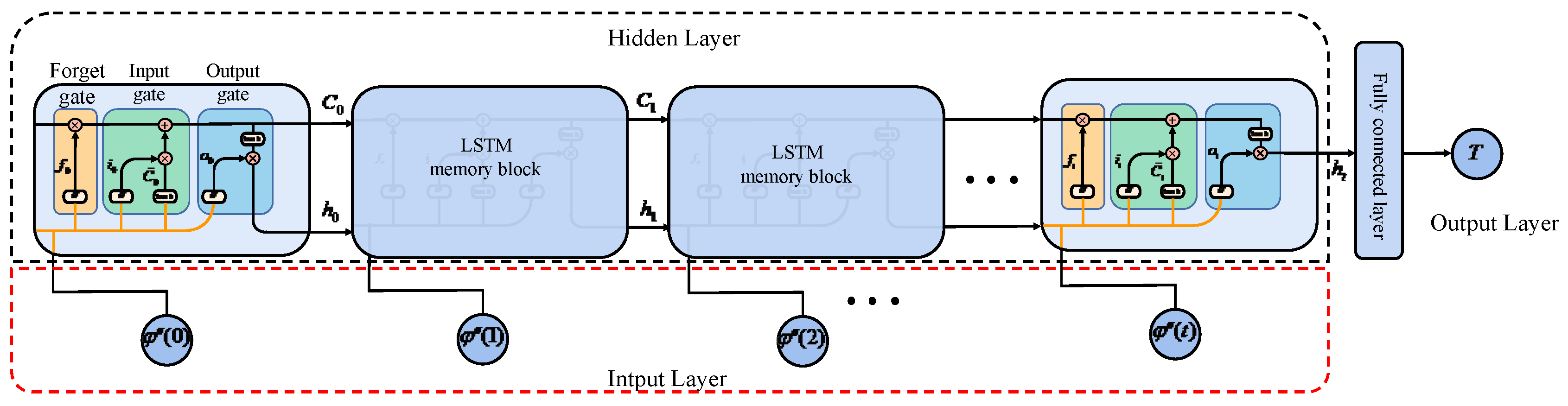
3.2. LSTM Demodulation Model

Based on the above training data, we could construct the corresponding LSTM model to learn the nonlinear relationship between phase signals and temperature, so as to avoid problems such as an inconsistent spectral ratio and the phase difference not being 120°, which affect the demodulation performance of temperature. The LSTM network is stacked as follows: input gate, forget gate, and output gate. First, the forget gate f_t determines which piece of information should be erased or retained in memory. Then, the input gate i_t evaluates the data within the input that have potential relevance and selects which portions of such information should be used and preserved. The next step involves updating long-term memory by integrating information from both the forget gate f_t and the input gate i_t via the cell state C_t. Finally, the hidden state h_t is computed by the output gate o_t, the cell state C_t, and the previous hidden state h_t-1. We designed the demodulation model to consist of an input layer, an LSTM hidden layer, a fully connected layer, and an output layer. The LSTM structure used in this paper is shown in Figure 4.

The LSTM hidden layer and fully connected layer in Figure 4 can effectively learn the characteristic information between phase signals and temperature. Based on the composition of the training data in the previous chapter, we selected three phase signals as the input and one temperature value as the output. Therefore, the number of input and output layers was three and one, respectively. Based on the experience of parameter selection of LSTM neural networks, we selected the number of neurons in the LSTM hidden layer to be 75. Since the fully connected layer implements the regression function, the number of neurons is consistent with the number of neurons in the LSTM hidden layer, which is 75. In addition, weight training in LSTM networks involves the use of the error backpropagation algorithm, which includes parameters such as learning rate and number of iterations. We set the learning rate of the LSTM network to 0.01 and the number of iterations to 50.

3.3. ABC-LSTM Demodulation Model

Since the initial weights and thresholds of LSTM networks are randomly initialized, this can lead to the possibility of being stuck in local minima, which affects the demodulation results. We used the artificial bee colony algorithm (ABC) to optimize the initial weights and thresholds of the LSTM network. ABC is a global optimization algorithm proposed by Karaboga to be implemented by simulating the nectar collection behavior of bee colonies [17]. In the process of optimizing initial weights and thresholds, the detailed steps are described as follows:

(1) Construction of the LSTM model. This model is used to assign the model weights and calculate the predictive output $T\left(t\right)$ based on weights and biases, such that $T\left(t\right)=f(\sum _{k=1}^n\mathrm{f}({\sum }_{i=1}^m\mathrm{f}({\sum }_{j=1}^o{u}_{ij}·{\phi }_j(t)+q_{i}T(t-1)+b_i)·{\omega }_{ik})·v_k+b)$, where n is the number of neurons in the fully connected layer, m is the number of neurons in the LSTM layer, O is the number of neurons in the input layer, $u_{ij}$, $q_i$ is the weight of the input layer, $b_i$ is the biases of the input layer, ${\omega }_{ik}$ is the weight of the LSTM layer, $v_k$ is the weight of the fully connected layer, and b is the biases of the fully connected layer.

(2) Initialize the parameters of ABC algorithm. The number, NS, of initial solutions, the limit value, and the maximum cycle number are set, where all initial solutions are D-dimensional vectors. D is the total number of weights and biases in the LSTM network.

(3) The initial solutions X fitness values are given by

$$MAE=\frac{1}{n}{\displaystyle {\sum }_{i=1}^n\left|Act{T}_i-Pre{T}_i\right|}$$

(8)

$$f(X)=\{\begin{array}{cc}1& MAE=0\\ \frac{1}{MAE+1}& MAE>0\end{array}$$

(9)

According to the fitness function, a fitness value of 1 indicates that the weight training error of the network is minimal, and the algorithm search produces the global optimal solution.

(4) Update the solution. If the updated solution shows better fitness than the previous solution, the new solution is used to replace the old solution. Otherwise, the number of update failures on the old solution increases by one until it reaches the maximum number of update solutions.

(5) Through the above iterations to the maximum cycle number, the optimal solution obtained is used as the initial parameters of the LSTM network for temperature demodulation.

According to the above ABC optimization LSTM neural network process, we need to set the parameters of the colony algorithm: the number of initial solutions, the maximum limit number of update solutions, and the maximum cycle number. (1) As the number of initial solutions increases, the potential for a more abundant source of nectar grows, allowing greater use of the global search capability of the artificial bee colony algorithm. However, if the number of initial solutions exceeds a certain threshold, the amount of iterative computation and time required will increase significantly without improving the algorithm’s solution performance. To ensure rapid convergence, we set the number of initial solutions at 50. (2) Setting the maximum limit number of update solutions will affect both the convergence rate and computational workload. We usually set the number at 10. (3) The ABC algorithm aims to identify the optimal solution through iterative optimization performed by the employed bee, onlooker bee, and scout bee stages. The maximum number of cycles is set at 20.

4. Experimental Setup and Results

To verify the demodulation performance of the ABC-LSTM model, we performed tests using a high-precision automatic measurement and verified these with a constant-temperature water tank ((SHUNMATECH, RTS-0515) RTS-0515) with a working tank opening of 235 × 180 mm² and a depth of 200 mm. The measurement system consisted of a narrow linewidth laser (DFB-M-1550-150-F-10-09MPF-FC/APC) with a central wavelength of 1550 nm and a bandwidth of 3 kHz, an AOM (Gooch&Housego, T-M200-0.1C2J-3-F2S) with a pulse frequency of 20 Hz and a pulse width of 20 ns, an EDFA (HOYATEK, HY-EDFA-C-22-M-FA), three PDs (KTC, KG-200M-APR) with a 200 MHz detection bandwidth, and a data acquisition card (NI, PXIe5170R) with a 250 MSa/s sampling rate. The sampling rate of the system signal was set to 20 Hz. We set up the sensing unit with a grating spacing of 50 m, coiled around a copper pipe with a diameter of 6 cm and a height of 15 cm. The first dataset was selected as test set 1 in an environment where the temperature was raised from 25.00 °C to 25.50 °C with an interval of 0.10 °C. Figure 5 shows three raw interference signals obtained from the outputs of three PD-acquired 3 × 3 couplers in a testing environment with a temperature range of 25.00–25.50 °C.

Using the innovative arctangent algorithm and phase unwrapping introduced in this article as a preprocessing step for the three interference signals mentioned above, the three phase signals obtained from the preprocessing, ${\phi }_1^{″}\left(t\right)$, ${\phi }_2^{″}\left(t\right)$,$\mathrm{a}\mathrm{n}\mathrm{d}{\phi }_3^{″}\left(t\right)$, were used as the output of the ABC-LSTM network, and the temperature result was obtained as shown in Figure 6. As shown in Figure 6, test set 1 was used to compare and display the demodulation results of the conventional passive 3 × 3 coupler method, the LSTM model, the ABC-LSTM model, and thermocouple sensor; the demodulated temperature increased from 25.00 °C to 25.50 °C as the time increased, as expected. Figure 6 displays the results of all the demodulation methods and real temperature values in increments of 0.10 °C, ranging from 25.00 °C to 25.50 °C. From the point marked by the triangle in Figure 6, an observation can be made regarding the temperature fluctuation that occurred, starting at 25.20 °C and increasing to 25.30 °C before ultimately stabilizing. This fluctuation was due to the implementation of the PID algorithm [18] used by the RTS-0515 temperature controller. Upon reaching the set temperature, the controller initiates a process of stopping the heating, resulting in the above-mentioned phase change in temperature. This process can also be observed through the results of the thermocouple temperature sensor. At the same time, this phenomenon shows the high resolution of the demodulation algorithm.

To further demonstrate the accuracy of demodulation achieved using the proposed approach, the absolute error in temperature during the five phases of constant temperature (25.10 °C, 25.20 °C, 25.30 °C, 25.40 °C, and 25.50 °C) is illustrated in Figure 7. The demodulation results obtained via the conventional passive 3 × 3 coupler method, elliptical fitting method, LSTM model, and ABC-LSTM model are presented in terms of absolute error. It should be noted that the five significant mutation errors in Figure 7 correspond to the triangle recognition error in Figure 6, which is explained in the description of Figure 6. As the temperature stabilized, the error in all four demodulation algorithms was relatively reduced. The absolute error of the traditional passive 3 × 3 coupler method was about 0.01 °C. The absolute errors of the ellipse fitting and LSTM models were significantly better than those of the traditional algorithm. This shows that the LSTM network can overcome the shortcomings of traditional algorithms and achieve the requirement of improving demodulation accuracy. However, the error curve of this method (with a maximum absolute error of about 0.0080 °C) was slightly higher than that of the ellipse fitting algorithm (with a maximum absolute error of about 0.0050 °C). The reason for this may be that the BP algorithm used by the LSTM network is prone to fall into local minima, which prevents the constructed nonlinear model from reaching the optimal solution. After optimization with the ABC algorithm, the overall error of the LSTM network was less than 0.0050 °C, which is significantly better than that achieved with the LSTM model and even the elliptical fitting. This result verifies the clear effectiveness of the ABC algorithm in optimizing the LSTM network.

To demonstrate the stability and adaptability of the proposed approach under consistent temperature conditions over an extended period, the second dataset was selected as test set 2 in an environment where the temperature was maintained at 25.00 °C for 200 min. According to Lisa’s analysis, the ellipse fitting algorithm requires certain limiting conditions to achieve signal demodulation. For example, the phase difference between two interference signals needs to change in real time. In the case of static measurements, the phase difference between two interference signals is a constant value, which can only form many repetitive points and does not meet the conditions for ellipse fitting. Therefore, we compared and analyzed three demodulation algorithms in a static experiment. As illustrated in Figure 8, it is evident that each demodulation technique exhibited a distinct performance at a temperature of 25.00 °C.

Figure 9 shows the absolute error distribution for the three algorithms. The error range was divided into 19 groups, each with a group interval of 0.0005 °C. The smallest group ranged from 0 to 0.0005 °C, while the largest group ranged from 0.0090 °C to 0.0095 °C. Starting from the 10th group, the ABC-LSTM algorithm exhibited no counts for absolute error demodulation. This illustrates that the proposed algorithm’s maximum absolute error does not exceed 0.0045 °C. Likewise, starting from the 17th group, the LSTM algorithm showed no counts for absolute error demodulation, indicating that the maximum absolute error of this algorithm does not exceed 0.0080 °C, which is smaller than the maximum absolute error of the conventional algorithm (0.0095 °C). Based on these results, we can infer that the ABC-LSTM demodulation model is preferable to the conventional and LSTM models, respectively. The figure also shows the kernel density curves of the three algorithms, which mainly describe the probability of each error point. From that, we can see that during the constant temperature measurement of 25.00 °C, errors for the three demodulation algorithms primarily ranged from 0 to 0.0025 °C. Furthermore, compared with the conventional passive 3 × 3 coupler method (0.0023 °C) and LSTM model (0.0019 °C), the mean absolute error of the proposed algorithm was the smallest at approximately 0.0014 °C. In conclusion, the ABC-LSTM demodulation model can accurately learn how the three interference signals change with temperature and has a higher stability than the other two models.

5. Discussions

In this study, an ABC-LSTM network was used to achieve temperature demodulation based on a 3 × 3 coupler optical system. This is the first time a neural network algorithm has been used to solve the problem of non-ideal phase differences between the three output signals, which are caused by the inconsistent splitting ratio of a 3 × 3 coupler and affect the demodulation performance of traditional algorithms. In dynamic experiments, we compared the proposed LSTM model and ABC-LSTM model with the traditional algorithm and ellipse fitting algorithm. From the demodulation results, it was found that the ellipse fitting algorithm had a significantly better demodulation performance in each temperature stage (maximum absolute error of 0.0050 °C) than the traditional algorithm (maximum absolute error of 0.0100 °C). This result indicates that the ellipse fitting algorithm is also suitable for dynamic temperature demodulation. The LSTM model, with a maximum absolute error of 0.0008 °C, presents certain advantages over traditional algorithms. It establishes the nonlinear relationship between phase signals obtained under non-ideal 3 × 3 coupler conditions and the corresponding temperature. This is similar to the ellipse fitting algorithm, both of which overcome the limitations of traditional algorithms that overlook the splitting ratios and phase differences of the non-ideal 3 × 3 coupler. Although the LSTM model shows promise in temperature demodulation, its effectiveness lags slightly behind that of the ellipse fitting algorithm. This is mainly because the neural network using the BP algorithm is prone to local minima, preventing the constructed nonlinear model from reaching the optimal value [11]. Research [12] has confirmed that the ABC algorithm can successfully optimize the initial parameters of the neural network, which is why we used it to enhance the LSTM model. The overall error of the ABC-LSTM model was less than 0.0050 °C, which is significantly better than that of the LSTM model. This result verifies the clear effectiveness of the ABC algorithm in optimizing the LSTM network. The ABC-LSTM network exhibited a superior demodulation performance compared to ellipse fitting. This can be attributed to the sensitivity of the latter algorithm to background and environmental noise, resulting in inaccurate fitting parameters and reduced demodulation accuracy. In contrast, the ABC-LSTM network employs three input variables and leverages their strong correlation with the output signal to mitigate the impact of noise on its output. Thus, the demodulation effect of the network is more robust and reliable. According to Lissajou analysis, fitting two interference signals into an ellipse requires specific conditions, including that the phase difference between the interference signals changes in real time. For static environments, the phase difference between the two interfering signals is constant, instead of satisfying ellipse fitting conditions. Therefore, ellipse fitting algorithms are more suitable for demodulating dynamic signals, such as vibration signals [19], than static demodulation. In our static experiments, we carried out a comparative analysis of the ABC-LSTM model, the LSTM model, and the conventional method. The error analysis graph (Figure 9) shows that the ABC-LSTM model performed similarly to other models at certain temperature points. However, in most cases, the demodulation error of the ABC-LSTM model was significantly smaller than that of the LSTM model and the traditional demodulation algorithm, which is consistent with the conclusion of the error distribution of neural network demodulation results described in reference [15]. Based on the above analysis, the ABC-LSTM model is also suitable for static temperature measurements and exhibits an excellent demodulation performance. However, it is worth noting that neural network algorithms entail a higher workload compared to traditional algorithms. This is due to the fact that neural network algorithms require building different network models in advance to adapt to different measured variables for optimal demodulation effects. Conversely, the traditional algorithm does not require the construction of additional models to achieve demodulation. Nevertheless, the performance advantages of the ABC-LSTM model over other models justify the additional resources required to implement it.

6. Conclusions

In this paper, a novel arc-tangent method based on a 3 × 3 coupler and a demodulation algorithm combining LSTM with ABC are proposed. The arc-tangent algorithm optimizes the input phase signal of the ABC-LSTM network model, establishing the relationship between the phase signal and temperature. The proposed ABC-LSTM method achieves high-resolution measurements with a temperature increment of 0.10 °C, demonstrating an absolute error of less than 0.0040 °C within the temperature range of 25.00 °C to 25.50 °C. To demonstrate the stability and adaptability of our method under long-term constant temperature conditions, we conducted measurements for approximately three hours in a temperature-controlled environment at 25.00 °C. The experimental results indicate that the ABC-LSTM method had a maximum error of 0.0045 °C, exceeding the conventional algorithm with an error of 0.0095 °C and the LSTM method with an error of 0.0080 °C. These results are consistent with the error performance observed under dynamic measurements, emphasizing the adaptability and effectiveness of the proposed algorithm. In addition, when comparing the average error values of the conventional passive 3 × 3 coupler method (0.0023 °C), LSTM model (0.0019 °C), and ABC-LSTM model (0.0014 °C), it is evident that ABC-LSTM method produces the most stable demodulation results. Therefore, the proposed method provides a new solution to improve demodulation performance in interferometric temperature sensors.

References

1. Liu, W.; Wu, X.; Zhang, G.; Li, S.; Zuo, C.; Fang, S.; Yu, B. Refractive index and temperature sensor based on Mach-Zehnder interferometer with thin fibers. Opt. Fiber Technol. 2020, 54, 102101. [Google Scholar] [CrossRef]
2. Chen, M.Q.; Zhao, Y.; Xia, F.; Peng, Y.; Tong, R.J. High sensitivity temperature sensor based on fiber Air-Microbubble Fabry-Perot interferometer with PDMS-filled hollow-core fiber. Sens. Actuators A Phys. 2018, 275, 60–66. [Google Scholar] [CrossRef]
3. Gao, S.; Ji, C.; Ning, Q.; Chen, W.; Li, J. High-sensitive Mach-Zehnder interferometric temperature fiber-optic sensor based on core-offset splicing technique. Opt. Fiber Technol. 2020, 56, 102202. [Google Scholar] [CrossRef]
4. Li, Y.; Wang, Y.; Xiao, L.; Bai, Q.; Liu, X.; Gao, Y.; Zhang, H.; Jin, B. Phase Demodulation Methods for Optical Fiber Vibration Sensing System: A Review. IEEE Sens. J. 2022, 22, 1842–1866. [Google Scholar] [CrossRef]
5. Park, S.; Rim, S.; Kim, Y.; Lee, B.H. Noncontact Photoacoustic Imaging Based on Optical Quadrature Detection with a Multiport Interferometer. Opt. Lett. 2019, 44, 2590–2593. [Google Scholar] [CrossRef] [PubMed]
6. Pang, Y.; Liu, H.; Zhou, C.; Huang, J.; Gu, H.; Zhang, Z. Pretreatment of Ultra-Weak Fiber Bragg Grating Hydrophone Array Based on Cubic Spline Interpolation Using Intensity Compensation. Sensors 2022, 22, 6814. [Google Scholar] [CrossRef] [PubMed]
7. Fan, P.; Yan, W.; Lu, P.; Zhang, W.; Zhang, W.; Fu, X.; Zhang, J. High sensitivity fiber-optic Michelson interferometric low-frequency acoustic sensor based on a gold diaphragm. Opt. Express 2020, 28, 25238–25249. [Google Scholar] [CrossRef] [PubMed]
8. Feng, S.; Chen, Q.; Gu, G.; Tao, T.; Zhang, L.; Hu, Y.; Yin, W.; Zuo, C. Fringe pattern analysis using deep learning. Adv. Photonics 2019, 1, 025001. [Google Scholar] [CrossRef]
9. Sun, Y.; Bian, Y.; Shen, H.; Zhu, R. High-accuracy simultaneous phase extraction and unwrapping method for single interferogram based on convolutional neural network. Opt. Lasers Eng. 2022, 151, 106941. [Google Scholar] [CrossRef]
10. Yu, D.; Qiao, X.; Wang, X. Light intensity optimization of optical fiber stress sensor based on SSA-LSTM model. Front. Energy Res. 2022, 10, 1265. [Google Scholar] [CrossRef]
11. Qian, L.; Zheng, Y.; Li, L.; Ma, Y.; Zhou, C.; Zhang, D. A New Method of Inland Water Ship Trajectory Prediction Based on Long Short-Term Memory Network Optimized by Genetic Algorithm. Appl. Sci. 2022, 12, 4073. [Google Scholar] [CrossRef]
12. Zhang, Y.; Zhang, Y.; He, K.; Li, D.; Xu, X.; Gong, Y. Intelligent feature recognition for STEP-NC-compliant manufacturing based on artificial bee colony algorithm and back propagation neural network. J. Manuf. Syst. 2022, 62, 792–799. [Google Scholar] [CrossRef]
13. Brown, D.A.; Cameron, C.B.; Keolian, R.M.; Gardner, D.L.; Garrett, S.L. Symmetric 3 × 3 Coupler-Based Demodulator for Fiber Optic Interferometric Sensors. Oe Fiber-dl Tentative; International Society for Optics and Photonics: Bellingham, WA, USA, 1991. [Google Scholar]
14. Coifman, R.R.; Steinerberger, S. Nonlinear Phase Unwinding of Functions. J. Fourier Anal. Appl. 2017, 23, 778–809. [Google Scholar] [CrossRef]
15. Wang, L.; Liu, H.; Pan, Z.; Xu, Y.; Fan, D.; Zhou, C.; Li, Y. Temperature demodulation for optical fiber F-P sensor based on DBNs with ensemble learning. Opt. Laser Technol. 2023, 162, 109275. [Google Scholar] [CrossRef]
16. Park, S.; Lee, J.; Kim, Y.; Lee, B.H. Nanometer-Scale Vibration Measurement Using an Optical Quadrature Interferometer based on 3 × 3 Fiber-Optic Coupler. Sensors 2020, 20, 2665. [Google Scholar] [CrossRef] [PubMed]
17. Ben Djaballah, C.; Nouibat, W. A new multi-population artificial bee algorithm based on global and local optima for numerical optimization. Clust. Comput. 2022, 25, 2037–2059. [Google Scholar] [CrossRef]
18. Lv, Y.; Niu, C.H.; Li, Y.Q.; Chen, Q.S.; Li, X.Y.; Liu, H. Precision Temperature Control System Based on PID Algorithm. Appl. Mech. Mater. 2013, 389, 483–488. [Google Scholar]
19. Zhang, W.; Lu, P.; Qu, Z.; Zhang, J.; Wu, Q.; Liu, D. Passive homodyne phase demodulation technique based on LF-TIT-DCM algorithm for interferometric sensors. Sensors 2021, 21, 8257. [Google Scholar] [CrossRef] [PubMed]
Figure 1. FBG-FP temperature-sensing system.
Photonics 10 01157 g001
Figure 2. (a) The simulation results of three normalized unwrapped phase signals. (b) Details of the normalized unwrapped phase signals in the heating state. (c) Details of normalized unwrapped phase signals at constant temperature.
Photonics 10 01157 g002
Figure 3. (a) Three normalized unwrapped phase signals. (b) Details of the normalized unwrapped phase signals.
Photonics 10 01157 g003
Figure 4. Structure of the LSTM.
Photonics 10 01157 g004
Figure 5. (a) The three measured interference signals were obtained at a temperature range of 25 to 25.5 °C, with an interval of 0.1 °C. (b) Detailed diagram of Figure 5a.
Photonics 10 01157 g005
Figure 6. The temperature increased from 25.00 °C to 25.50 °C, demodulated using the conventional NPS method, LSTM model, ABC-LSTM model, and elliptical fitting method.
Photonics 10 01157 g006
Figure 7. Absolute value errors of four algorithms.
Photonics 10 01157 g007
Figure 8. The temperature at 25.00 °C, demodulated using the conventional NPS method, LSTM model, ABC-LSTM model.
Photonics 10 01157 g008
Figure 9. The distribution of the absolute error of the three algorithms at a consistent temperature.
Photonics 10 01157 g009
Disclaimer/Publisher’s Note: The statements, opinions and data contained in all publications are solely those of the individual author(s) and contributor(s) and not of MDPI and/or the editor(s). MDPI and/or the editor(s) disclaim responsibility for any injury to people or property resulting from any ideas, methods, instructions or products referred to in the content.