Experimental Investigations and Modeling of Interference Fringe Geometry in Line-Shaped Gaussian Beam Intersections for Laser Doppler Sensors

Abstract

Line-shaped beam-based Doppler distance sensors enable 3D shape measurements of rotating objects, for instance for working lathe monitoring with a simultaneous, multipoint velocity, and distance measurement. The velocity and distance estimations are fundamentally referred to the interference fringe spacing of the sensors. In this case, the fringe spacing variation-caused measurement error is significant; however, a complete, accurate model of the fringe geometry distribution for the line-shaped fringe volume is still missing and required to identify and minimize the error. Therefore, this work presents a high-accuracy 3D model for the fringe spacing evaluation of the sensors with experimental investigations. The model is derived from the phase expression of Gaussian beams introducing extension ratio, and can be universally applied to describe fringe geometry distribution throughout the intersection volume of spherical and line-shaped beams. With an experimental setup of a laser Doppler sensor, a full-field fringe spacing estimation using a high-resolution matrix camera is performed with dual-wavelength beams. The numerical modeling and experimental results show an average relative difference below $0.6\%$.

1. Introduction

The simultaneous optical in-process measurement of the velocity and distance of moving objects is a significant task in diverse applications, such as moving rough surfaces and tracer particles’ monitoring for workpiece shape measurements in turning lathes and flow phenomena detections of microfluidics. For this purpose, a novel laser Doppler distance sensor is developed [1,2,3]. Compared to conventional optical distance measurement techniques [4,5,6,7,8,9,10,11], it offers the advantage of simultaneous axial distance and lateral velocity measurement based on two interference fringe systems by superimposing dual-wavelength Gaussian beams. In this sensor, the velocity and distance are respectively determined from the Doppler frequency and phase difference of the speckle signals generated by optically rough surfaces or particles passing through the fringe systems. The Doppler frequency and phase difference of the speckle signals are fundamentally referred to the fringe spacing [12]. Therefore, in order to obtain an accurate measurement, a significant step is to achieve accurate, full-field fringe spacing distribution in the intersection volume.

With the birth of lasers [13,14], the laser beam with a Gaussian intensity profile is perhaps the most important one, which is often called the Gaussian beam and the fundamental mode as compared to the higher order modes [15]. The Gaussian beam is widely used in the research and application of laser devices [16,17], optical processing, and measurement [18,19]. The Gaussian intensity profile of the beams is determined by diffraction effects. Historically, the modes were approximated by wave beams, and the concept of electromagnetic wave beams was introduced by investigating the properties of sequences of lenses for the transmission of electromagnetic waves. The resonant properties of Gaussian beams in the resonator structure, the propagation characteristics in free space, and the behaviors as they interact with diverse optical systems have been investigated since the 1960s [15]. As limitations of the early research, the investigations of Gaussian beams mainly focused on the passage of paraxial rays through optical elements, the wave nature of the beams, and diffraction effects. With the development of laser measurement techniques, the study of Gaussian beams needs to be combined with practical applications. Especially for the dual-beam laser Doppler sensing, the influence of the properties of Gaussian beams on the interference field urgently needs to be investigated and quantified for improving measurement accuracy.

In dual Gaussian beam interference, the effect of beam nature on the variation of fringe spacing in the intersection volume is significant due to its potential impact on the applications. In the initial fringe field analyses of the intersection volume, the valid expressions were derived for the variation in fringe spacing along the probe volume longitudinal axis and along the transverse axis perpendicular to the fringes [20]. An alternative expression is deduced for the transverse variation and the longitudinal model is extended by referring the results to system parameters [21]. The resulting equations are effective for evaluating the longitudinal fringe spacing only when the beam waists are far from the center of intersection volume. They are not valid under a relatively good alignment, which is the condition of greatest interest and most uses. The above works all contain multiple approximations whose effects are hard to quantify. In another way, an indirect fringe distortion inspection by using signal frequency error analysis was proposed considering various system parameters such as the beam crossing angle and the lens focal length [22]. But the formulas obtained are not feasible with simple computation and the synergism of these parameters on the fringe variation are still unclear. With further improvement, the valid expressions of fringe spacing throughout the intersection volume of two Gaussian beams were performed, which can be simplified by means of precisely quantified approximations for an easy calculation [23]. But the expressions describe the longitudinal or transverse variation of fringe geometry independently and are only applicable to spherical Gaussian beams. Up to now, a universal, accurate 3D model of the fringe spacing distribution in the intersection volume is still missing and required. Especially for the laser Doppler distance sensor with line-shaped beam based multipoint measurement [24], the fringe geometry change along the height of the intersection volume leads to a great systematic error and therefore needs to be exactly investigated and computed to eliminate the error.

The aim of this paper is to present an exact, universal model of fringe spacing distribution for calibrating the interference fringe field in paraxial Gaussian beam intersections. A comprehensive analysis resulting in accurate 3D expressions for the fringe spacing is conducted first in Section 2. The expressions refer to system parameters relevant to the optics configuration, enabling a priori evaluation of fringe variation for system optimization. To demonstrate the model, an experimental setup of the laser Doppler system is developed and a full-field fringe spacing evaluation is performed with line-shaped beams in two wavelengths. With the consistent condition, the numerical modeling of fringe spacing is conducted and the relative differences of the modeling and experimental results are investigated in Section 3.

2. Model of Fringe Geometry

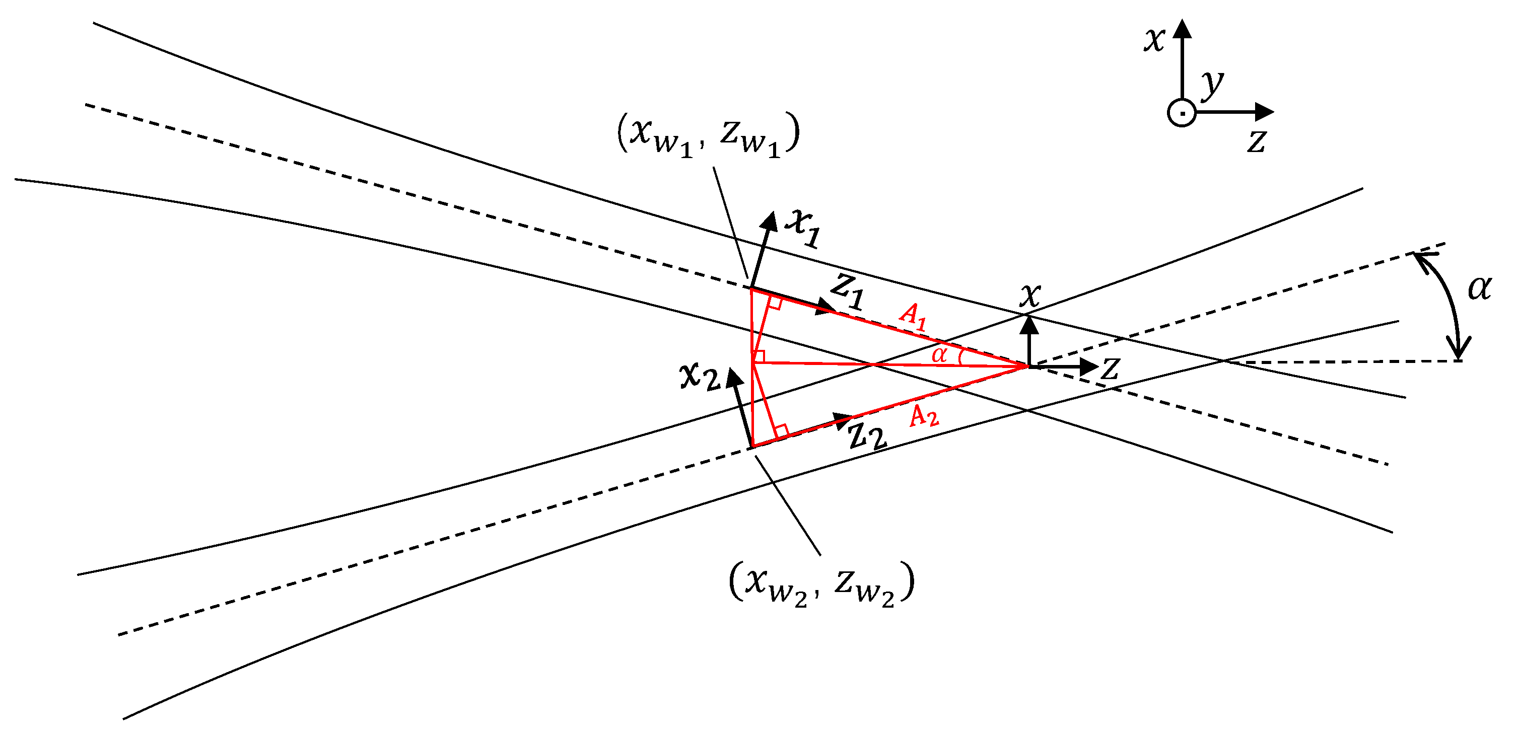
The dual-beam mode is an optical method that is widely used in laser Doppler sensors for generating Doppler frequency-modulated scattered light signals, cf. Figure 1. In this mode, two Gaussian beams from coherent light sources are superimposed to form an interference fringe volume, which offers a fundamental dimension for the following analysis of fringe spacing. For a global, intuitive observation and analysis, the coordinate transformation from the independent coordinates of the two beams to the beam intersection volume coordinate is essential.

In the intersection volume, the interference is generated by two beams crossing with a half angle $\alpha$. $x_i$, $y_i$, and $z_i$ are defined as coordinates in the beam coordinate system with its origin at the waist of beam i. The position in the range of the intersection volume is described by the x, y, z coordinate system, the origin of which is at the intersection of the two beam centerlines. $x_{w_i}$ and $z_{w_i}$ are the waist coordinates of beam i in the x, y, z coordinate system, which are also the origin coordinates of the $x_i$, $y_i$, $z_i$ coordinate system and constants for a certain dual-beam optical system. Based on the geometric relation, $A_1={-z}_{w_1}·cos\alpha +x_{w_1}·sin\alpha$, $A_2={-z}_{w_2}·cos\alpha -x_{w_2}·sin\alpha$. The transformation between $x_i$, $y_i$, $z_i$ and x, y, z for two beams can thus be achieved by rotation and translation:

$$\begin{array}{cc}\hfill & \left[\begin{array}{c}{x}_1\\ y_1\\ z_1\\ 1\end{array}\right]=\left[\begin{array}{cccc}1& 0& 0& 0\\ 0& 1& 0& 0\\ 0& 0& 1& A_1\\ 0& 0& 0& 1\end{array}\right]·\left[\begin{array}{cccc}cos\alpha & 0& sin\alpha & 0\\ 0& 1& 0& 0\\ -sin\alpha & 0& cos\alpha & 0\\ 0& 0& 0& 1\end{array}\right]·\left[\begin{array}{c}x\\ y\\ z\\ 1\end{array}\right],\hfill \\ \hfill & \left[\begin{array}{c}{x}_2\\ y_2\\ z_2\\ 1\end{array}\right]=\left[\begin{array}{cccc}1& 0& 0& 0\\ 0& 1& 0& 0\\ 0& 0& 1& A_2\\ 0& 0& 0& 1\end{array}\right]·\left[\begin{array}{cccc}cos\alpha & 0& -sin\alpha & 0\\ 0& 1& 0& 0\\ sin\alpha & 0& cos\alpha & 0\\ 0& 0& 0& 1\end{array}\right]·\left[\begin{array}{c}x\\ y\\ z\\ 1\end{array}\right],\hfill \end{array}$$

(1)

which then offer the coordinate relation:

$$\begin{array}{cc}\hfill & x_1=xcos\alpha +zsin\alpha ,y_1=y,\hfill \\ \hfill & z_1=-(x-x_{w_1})sin\alpha +(z-z_{w_1})cos\alpha ,\hfill \\ \hfill & x_2=xcos\alpha -zsin\alpha ,y_2=y,\hfill \\ \hfill & z_2=(x-x_{w_2})sin\alpha +(z-z_{w_2})cos\alpha .\hfill \end{array}$$

(2)

By the expression of the radiation field of Gaussian beams [25], the phase variation per meter $k=2\pi /\lambda$ and the beam Rayleigh range $z_{R_i}=\pi w_{0_i}^2/\lambda$, the phase of each beam is given as

$${\theta }_i(x,y,z)=-k{z}_i+{tan}^{-1}\frac{z_i}{z_{R_i}}-\frac{k}{2}\frac{x_i^2+y_i^2}{R\left(z_i\right)}.$$

(3)

The minimum radius of the beam at the beam waist is given by $w_{0_i}$. In Equation (3), the first two factors describe the phase propagation towards $z_i$. The last factor indicates the dependency of the phase on the lateral coordinates $x_i$ and $y_i$ as well as the phase curvature radius $R\left(z_i\right)$, which depends on $z_i$:

$$R\left(z_i\right)=z_i\left[1+{\left(\frac{z_{R_i}}{z_i}\right)}^2\right],$$

(4)

and the beam spot size is

$$w\left(z_i\right)=w_{0_i}\sqrt{1+{\left(\frac{z_i}{z_{R_i}}\right)}^2}.$$

(5)

Interference fringes in the scope of intersection volume originate from a constant phase difference and, thus, are expressed as

$$\begin{array}{cc}\hfill 2n\pi ={\theta }_1(x,y,z)-{\theta }_2(x,y,z)=& 2\pi [-\frac{1}{\lambda }(z_1-z_2)+\frac{1}{2\pi }\left({tan}^{-1}\frac{z_1}{z_{R_1}}-{tan}^{-1}\frac{z_2}{z_{R_2}}\right)\hfill \\ \hfill & -\frac{1}{2\lambda }\left(\frac{x_1^2+y_1^2}{R\left(z_1\right)}-\frac{x_2^2+y_2^2}{R\left(z_2\right)}\right)].\hfill \end{array}$$

(6)

Substituting Equations (2) and (4) into Equation (6) and differentiating with respect to x, the fringe spacing L yields

$$\begin{array}{cc}\hfill L={\left(\frac{dn}{dx}\right)}^{-1}=& \frac{\lambda }{2sin\alpha }[1-\frac{1}{2tan\alpha }\left(\frac{x_1{z}_1}{{z_1}^2+{z_{R_1}}^2}-\frac{x_2{z}_2}{{z_2}^2+{z_{R_2}}^2}\right)-\frac{z_{R_1}\lambda }{4\pi ({z_1}^2+{z_{R_1}}^2)}\hfill \\ \hfill & -\frac{z_{R_2}\lambda }{4\pi ({z_2}^2+{z_{R_2}}^2)}-\frac{x_1^2({z_1}^2-{z_{R_1}}^2)}{4{({z_1}^2+{z_{R_1}}^2)}^2}-\frac{x_2^2({z_2}^2-{z_{R_2}}^2)}{4{({z_2}^2+{z_{R_2}}^2)}^2}\hfill \\ \hfill & -\frac{y_1^2({z_1}^2-{z_{R_1}}^2)}{4{({z_1}^2+{z_{R_1}}^2)}^2}-\frac{y_2^2({z_2}^2-{z_{R_2}}^2)}{4{({z_2}^2+{z_{R_2}}^2)}^2}{]}^{-1}.\hfill \end{array}$$

(7)

Since Equation (6) is a composite function, it is inevitable to reintroduce $x_i$ and $z_i$ during the derivation. A derivation process is offered by Equations (A1)–(A3) in Appendix A. For a relatively concise expression, parameter replacement is not performed again for Equation (7). In most computer modeling conditions, combining Equation (2), the variables can be simply and quickly transformed.

Terms $\frac{x_i^2({z_i}^2-{z_{R_i}}^2)}{4{({z_i}^2+{z_{R_i}}^2)}^2}$ and $\frac{y_i^2({z_i}^2-{z_{R_i}}^2)}{4{({z_i}^2+{z_{R_i}}^2)}^2}$ are derived from the transverse phase terms in Equation (6) with respect to the phase curvature radius $R\left(z_i\right)$. The term $\frac{z_{R_i}\lambda }{4\pi ({z_i}^2+{z_{R_i}}^2)}$ is associated with the Guoy phase shift ${tan}^{-1}\frac{z_i}{z_{R_i}}$. As the added phase shift is greatest around the beam waist, term $\frac{z_{R_i}\lambda }{4\pi ({z_i}^2+{z_{R_i}}^2)}$ is maximized under ideal alignment conditions when $z_i\approx 0$. By substituting $z_i=0$ into the terms, it is seen that the maximum magnitude of the terms is equal to ${\lambda }^2/{\left(2\pi w_{0_i}\right)}^2$. In order for these terms to contribute more than $0.01\%$ to the fringe spacing, the beam waists must be less than 10 $\mathsf{\mu }$m with $\lambda =685$ nm and less than 7.5 $\mathsf{\mu }$m with $\lambda =500$ nm. Under most practical circumstances, the $\frac{z_{R_i}\lambda }{4\pi ({z_i}^2+{z_{R_i}}^2)}$ terms can thus be neglected. Regarding $\frac{x_i^2({z_i}^2-{z_{R_i}}^2)}{4{({z_i}^2+{z_{R_i}}^2)}^2}$ terms, the maximum of $x_i^2$ is determined by the square of beam radius $w^2\left(z_i\right)$, i.e., $w_{0_i}^2(1+\frac{z_i^2}{z_{R_i}^2})$. With $z_{R_i}=\pi w_{0_i}^2/\lambda$, the maximum of $\frac{x_i^2({z_i}^2-{z_{R_i}}^2)}{4{({z_i}^2+{z_{R_i}}^2)}^2}$ equals to ${\left(\frac{\lambda }{2\pi w_{0_i}}\right)}^2·\frac{{z_i}^2-{z_{R_i}}^2}{{z_i}^2+{z_{R_i}}^2}$, which is bounded by ${\lambda }^2/{\left(2\pi w_{0_i}\right)}^2$ as well, and therefore can be neglected.

For the laser Doppler sensor with line-shaped Gaussian beams and camera-based detection [12,24], the intersection volume is expended and sliced towards the y-axis for high-resolution, simultaneous multipoint measurement instead of single point measurement. Since the fringe spacing is variable for different measurement points along the y-axis, the fringe spacing variation enables a measurement uncertainty of a micron in a 3D shape measurement of a rotating object by uncertainty propagation, even if the relative variation is in the level of ${10}^{-3}$. Thus, the fringe spacing in each measurement point must be evaluated independently. The y-axis fringe spacing variation is therefore non-ignorable and needs to be exactly investigated and calculated to minimize the systematic error. In this case, as the solo terms depending on the y coordinate, the $\frac{y_i^2({z_i}^2-{z_{R_i}}^2)}{4{({z_i}^2+{z_{R_i}}^2)}^2}$ terms are significant for describing the fringe spacing. The radius of the beam waist is defined on the x- and y-axes by $w_{0x_i}$ and $w_{0y_i}$, respectively. In the interference region of the dual Gaussian beam mode, the fringe spacing is determined by the phase difference of the beams. Since the incident angle is in the x–z plane, the fringe spacing significantly depends on the phase difference along the x direction (fringe direction) and the z direction (optical axis). In this case, in the y direction, the beam waist and Rayleigh range variations, as well as the changes in phase curvature radius caused by them, have less to no influence on the fringe spacing compared to the spherical beam condition. Thus, introducing the y-axis extension ratio of the intersection volume $m=w_{0y_i}/w_{0x_i}$, and considering $y_1=y_2=y$, the Rayleigh range in the x direction $z_{R{x}_i}=z_{R_i}$, a 3D model of the fringe spacing can be expressed as

$$\begin{array}{cc}\hfill L=& \frac{\lambda }{2sin\alpha }[1-\frac{1}{2tan\alpha }\left(\frac{x_1{z}_1}{{z_1}^2+{z_{R{x}_1}}^2}-\frac{x_2{z}_2}{{z_2}^2+{z_{R{x}_2}}^2}\right)\hfill \\ \hfill & -\frac{1}{4}{\left(\frac{y}{m}\right)}^2\left(\frac{{z_1}^2-{z_{R{x}_1}}^2}{{({z_1}^2+{z_{R{x}_1}}^2)}^2}+\frac{{z_2}^2-{z_{R{x}_2}}^2}{{({z_2}^2+{z_{R{x}_2}}^2)}^2}\right){]}^{-1}.\hfill \end{array}$$

(8)

Employing Equation (8), the fringe geometry throughout the intersection volume of spherical beams and line-shaped beams along the y-axis can be evaluated for arbitrary sizes and positions of the two beam waists.

3. Results and Discussion

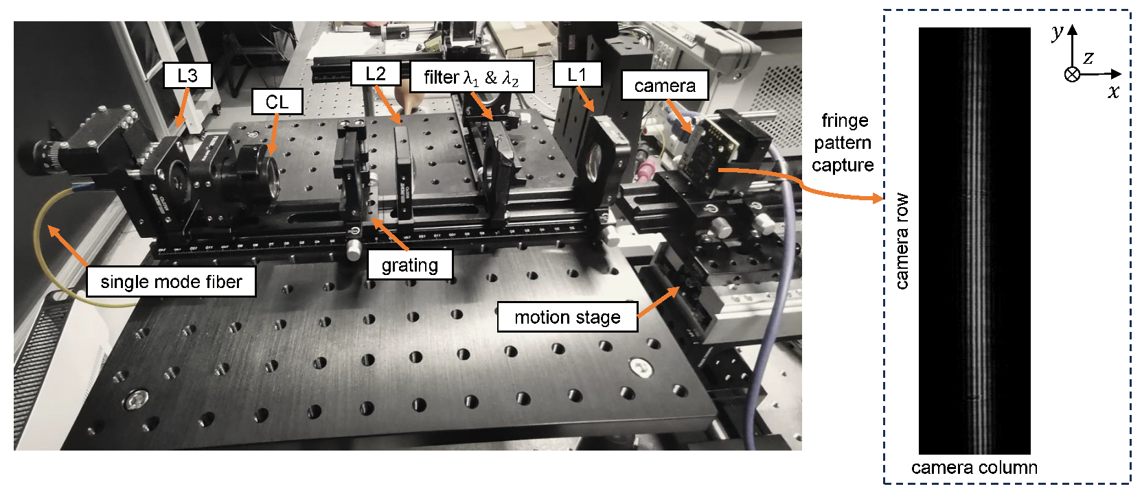
In the experimental investigations of the fringe field, a line-shaped beam-based laser Doppler velocity and distance sensor system is developed based on a Mach–Zehnder velocimeter [26,27] with beams of dual wavelength, cf. Figure 2.

The laser light with the wavelengths of ${\lambda }_1=685$ nm and ${\lambda }_2=659$ nm generated by two fiber-coupled laser diodes are coupled into a single mode fiber. Through the collimating lens L3, on the distal end of the fiber, the collimated beams are focused by the cylindrical lens CL with the focal lengths $f_{\mathrm{cx}}=50$ mm and $f_{\mathrm{cy}}=\infty$. Thereby, the beams remain parallel on the y-axis. A transmission diffraction grating with the grating constant $g=4$ $\mathsf{\mu }$m is positioned at the focal plane of CL and L2 to split the bichromatic light. One filter blocks the +1. diffraction order (DO) from ${\lambda }_1$ and the other one blocks the −1. DO from ${\lambda }_2$. The x-axis dimension of the 0. DO beams is about 25 $\mathsf{\mu }$m, and the gap of 1 mm between the two filters is made to allow the beams crossing. Passing the Keplerian telescope consisting of lens L1 and L2 ($f_1=80$ mm, $f_2=40$ mm), the remaining beams of ±1. and 0. DO are superimposed in the focal plane of L1 with a constant dimension on the y-axis. This produces two interference fringe systems around the beam waists with $L\approx$ 8 $\mathsf{\mu }$m, $2·w_{0y_i}\approx 2$ mm, $2·w_{0x_i}\approx 50$ $\mathsf{\mu }$m and, thus, m is about 40. The beam waist dimensions are obtained by using camera detection and geometric optics of the system parameters. This offers a condition of good alignment with the two beam waists located at the center of the intersection volume, i.e., $x_{w_1}=x_{w_2}=0$ and $z_{w_1}=z_{w_2}=0$, which is of most use. By using full-field, camera-based scattered light detection, the sensor allows a simultaneous measurement of up to several hundred points. Since the half angle $\alpha =\frac{1}{2}arctan\frac{f_2\lambda }{f_{1}g}$ and is small (below $5^{\circ }$), $sin\alpha \approx tan\alpha$ and Equation (8) can be written as

$$\begin{gathered} \begin{array}{c}\hfill L=\frac{f_{1}g}{f_2}{\left[1-\frac{f_{1}g}{f_2\lambda }\left(\frac{x_1{z}_1}{{z_1}^2+{z_{R{x}_1}}^2}-\frac{x_2{z}_2}{{z_2}^2+{z_{R{x}_2}}^2}\right) \\ \hspace{1em}\hspace{1em}\hspace{1em}\hspace{1em} -\frac{1}{4}{\left(\frac{y}{m}\right)}^2\left(\frac{{z_1}^2-{z_{R{x}_1}}^2}{{({z_1}^2+{z_{R{x}_1}}^2)}^2}+\frac{{z_2}^2-{z_{R{x}_2}}^2}{{({z_2}^2+{z_{R{x}_2}}^2)}^2}\right)\right]}^{-1}.\end{array} \end{gathered}$$

(9)

The fringe spacing varies with the change of position in the intersection volume due to the nature of Gaussian beams. For realizing a full-field fringe geometry evaluation of the extended intersection volume, a matrix camera (UI-1492LE, resolution H × V $=3840\times$ 2748 pixel, pixel size $D_{\mathrm{p}}=1.67$ $\mathsf{\mu }$m) is integrated onto a linear motion stage (MICOS LS-65, resolution 0.2 $\mathsf{\mu }$m) in front of the sensor system to detect the fringe pattern, cf. Figure 3. The modeling and data processing in this paper are conducted by using MATLAB.

The position of the camera towards the z-axis changes with the movement of the stage in a constant step size of 10 $\mathsf{\mu }$m. Note that the x, y, z coordinate system of the beam intersection volume is different from the sensor coordinate system of $x_{\mathrm{s}}$, $y_{\mathrm{s}}$, $z_{\mathrm{s}}$. The fringe pattern in each step is measured 10 times and is utilized to evaluate the fringe spacing in the amplitude spectrum employing the Fast Fourier Transform (FFT). Fringe spacing $L=\frac{1}{f_{\mathrm{f}}}·D_{\mathrm{p}}$ is then obtained based on the fringe number per pixel $f_{\mathrm{f}}$. The average relative measurement uncertainty of fringe spacing $0.34\%$ is obtained. According to the measurement principle of the laser Doppler sensors, the fringe spacings along the x-axis are averaged by the FFT for estimating the fringe spacings of y- and z-axes. The fringe patterns measured in the experiment and the fringe field processing along the y-axis are shown in Figure 4.

Figure 4a illustrates the fringe patterns achieved at the beam waist and the edge of the measurement range with the two wavelengths of 685 nm and 659 nm. The fringe field is sliced along the y-axis in pixels depicted in Figure 4b, which can be used for a simultaneous multipoint measurement. The fringe spacings are thus experimentally evaluated at various positions of the intersection volume in the range of 200 $\mathsf{\mu }$m on the z-axis and 2 mm on the y-axis. 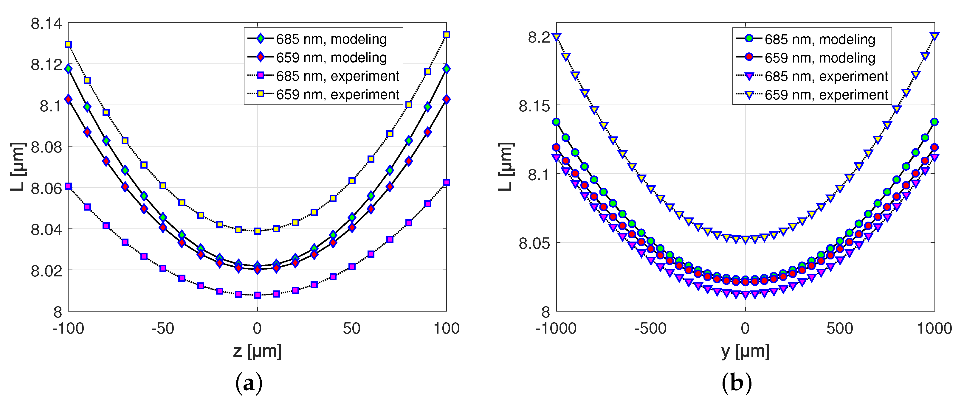Under the same conditions, the numerical modeling of fringe spacing based on Equation (9) is performed and compared with the experimental results in Figure 5.

It can be seen that the trends of fringe spacings in the modeling and experiment are comparable. As shown in Figure 5a, the fringe spacings of both wavelengths almost keep consistent in the range of −30 $\mathsf{\mu }$m to 30 $\mathsf{\mu }$m on the z-axis around the center of the measurement volume, which is the position of the beam waists and indicates that the sensor system has a good alignment. It shows that the fringe spacing varies in the range of 8.02 to 8.12 $\mathsf{\mu }$m in the modeling. At the edges, the fringe spacing differences of about 0.02 $\mathsf{\mu }$m are indicated between the two wavelengths. For the experimental results, the fringe spacing changes from 8.01 to 8.13 $\mathsf{\mu }$m, which is similar to the modeling results, and the maximum difference of around 0.07 $\mathsf{\mu }$m between both wavelengths is revealed. In Figure 5b, the fringe spacing along the y-axis illustrates a variation from 8.02 to 8.14 $\mathsf{\mu }$m with the modeling. The fringe spacing also shows the differences of about 0.02 $\mathsf{\mu }$m at the edges in the both wavelengths. In the experiment, the fringe spacing is in a variation range of 8.01 to 8.2 $\mathsf{\mu }$m and the maximum difference is about 0.08 $\mathsf{\mu }$m between the two wavelengths.

In the modeling, a fringe spacing difference of about 0.02 $\mathsf{\mu }$m from $\lambda /2sin\alpha$ around the center of beam waist results from the x-axis averaging. The full-field maps of fringe spacings are obtained in Figure 6.

All the modeling and experimental results manifest a homologous, inverted Gaussian-like distribution in which the fringe spacings around the bottom of the map are about 8 $\mathsf{\mu }$m. In the modeling, the fringe spacing can gradually increase to 9.3 $\mathsf{\mu }$m approaching the corner of the map. With the same coordinate range, the experimental results can reach 8.5 $\mathsf{\mu }$m. This is comparable with the Gaussian intensity distribution and, thus, suggests that the fringe spacing variation is determined by the characteristic of the Gaussian beams. The shift of the fringe spacing distribution in the experiment is due to a slight tilt between the camera’s surface and the optical axis. In order to investigate the accuracy of the model and the experiment, the relative differences between the modeling and experimental results at the same coordinates are estimated along the y- and z-axes, respectively, cf. Figure 7.

Figure 7a shows on the z-axis that the modeling results of both wavelengths offer tiny differences of below $0.33\%$, and for the experimental results they are below $0.74\%$. The relative differences between the modeling and experimental results with the same wavelength are all below $1.85\%$. Similarly, as depicted in Figure 7b, the modeling results of the two wavelengths gives the differences of below $0.34\%$ on the y-axis. For the experimental results, their upper limit is $0.71\%$. With the same wavelength, the relative differences between the modeling and experimental results are limited to less than $1.67\%$. Eventually, the average relative differences are evaluated and listed in

Table 1. Average relative differences in the numerical modeling and experiments with the two wavelengths.

	Average Relative Difference
Modeling of both wavelengths	$0.12\%$
Experiments of both wavelengths	$0.49\%$
Modeling and experiment of 659 nm	$0.53\%$
Modeling and experiment of 685 nm	$0.57\%$

.

This reveals that the average relative differences of the modeling and experimental results with wavelengths of 659 nm and 685 nm are all below $0.6\%$ and, thus, indicates that the method is feasible.

Figure 7 also shows that the relative differences in the experiment are a little higher than in the modeling. This is caused by the noise of the fringe images and the slight position difference of the camera for the two fringe volumes. For the modeling, the fringe spacing difference results from the difference in wavelength. In the experiment, the trend of relative difference is influenced by the light intensity as well. The decreasing light intensity results in lowering the signal-to-noise ratio (SNR) approaching the edge of the beam. Therefore, the difference between the modeling and the experiment has a relatively significant increase at both ends of the curves. The minor variation of the differences around the center of the curve is due to a position deviation of the experiment relative to the model. Overall, the tendencies of the relative differences are comparable.

4. Conclusions

A full-field 3D mathematical model and experimental investigation of the interference fringe geometry in the intersection of Gaussian beams are proposed for minimizing the systematic error of laser Doppler sensors. The model is derived from the phase expression of Gaussian beams by using the theory of partial differentiation and introducing extension ratio, thus, can be universally applied to spherical and line-shaped Gaussian beams with arbitrary beam waist sizes and positions.

Based on a laser Doppler sensor system, the experimental fringe spacing analysis is conducted with line-shaped beams in the two wavelengths of 659 nm and 685 nm. A matrix camera integrated on a high-precision motion stage is used to detect fringe patterns at various positions inside of the intersection volume. The fringe spacings are then evaluated by employing the Fast Fourier Transform (FFT) along the fringe direction. Utilizing the same conditions, the modeling results show the average relative differences of $0.53\%$ and $0.57\%$ compared to the experimental results with both wavelengths, respectively. Between both wavelengths, the average relative differences in the modeling and experimental results are $0.12\%$ and $0.49\%$, respectively. These validate the feasibility of the proposed methods.

As an outlook, the fringe geometry model can be further improved for arbitrary shaped Gaussian beams. The model refers to system parameters including focal length, wavelength, and grating constant for the dual-beam laser Doppler sensor configuration. It can offer a key priori knowledge of the appropriate parameters targeting different measurements that require a diverse measurement range, working distance, fringe spacing, etc. The model may also offer system design equations that identify the important parameters governing the fringe field uniformity. The limitation of systematic error is predictable by the model based on the modeled fringe geometry variation. Combined with fringe calibrations it allows for identifying alignment errors of the system for rapid system optimization. As a broad prospect, the model can be commonly applied to dual-beam interference sensors which are influenced by the nonuniform fringe field.