A Model-Based Approach for Measuring Wavefront Aberrations Using Random Ball Residual Compensation

 and
and
Abstract
:1. Introduction
2. Theoretical Analysis
- A.
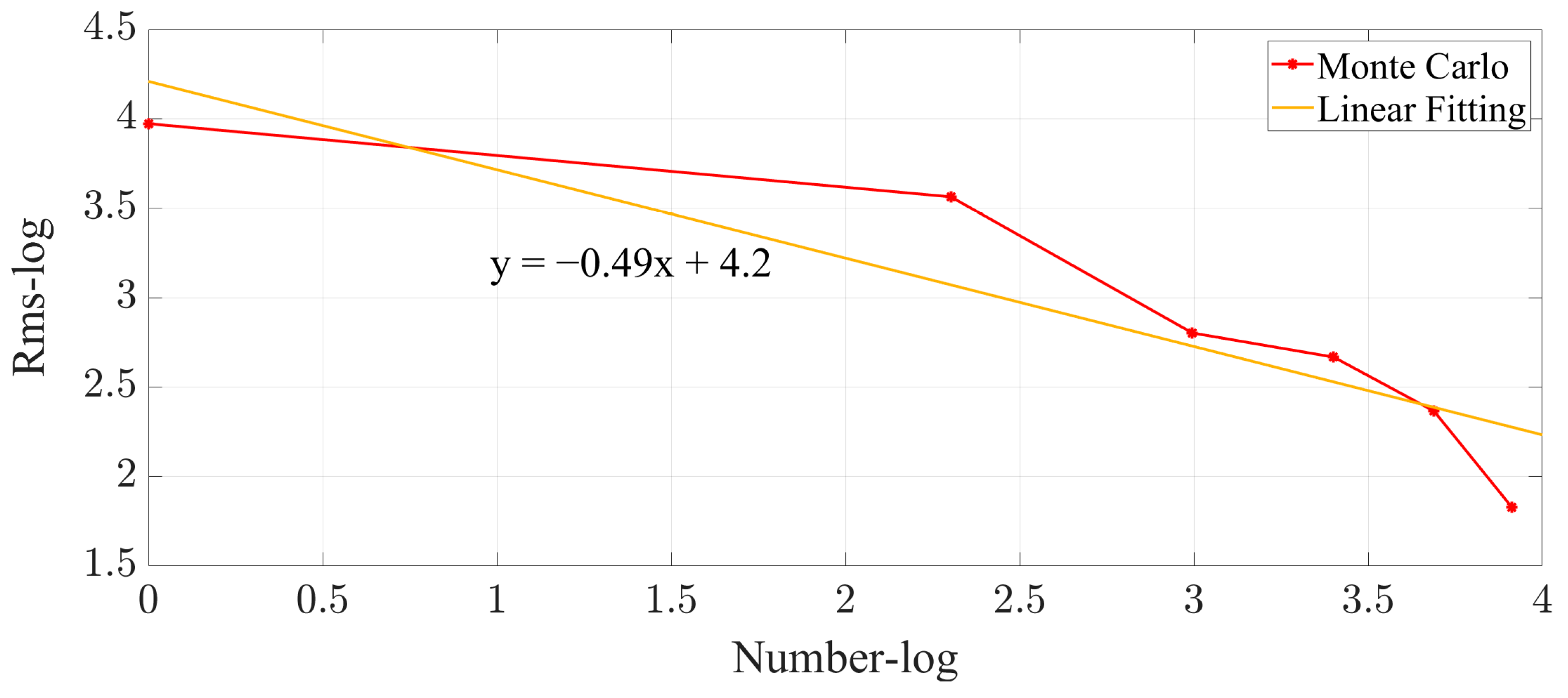
- Random averaging method
- B.
- High-precision measurement
- C.
- Model analysis
- D.
- Uncertainty analysis
3. Experiment
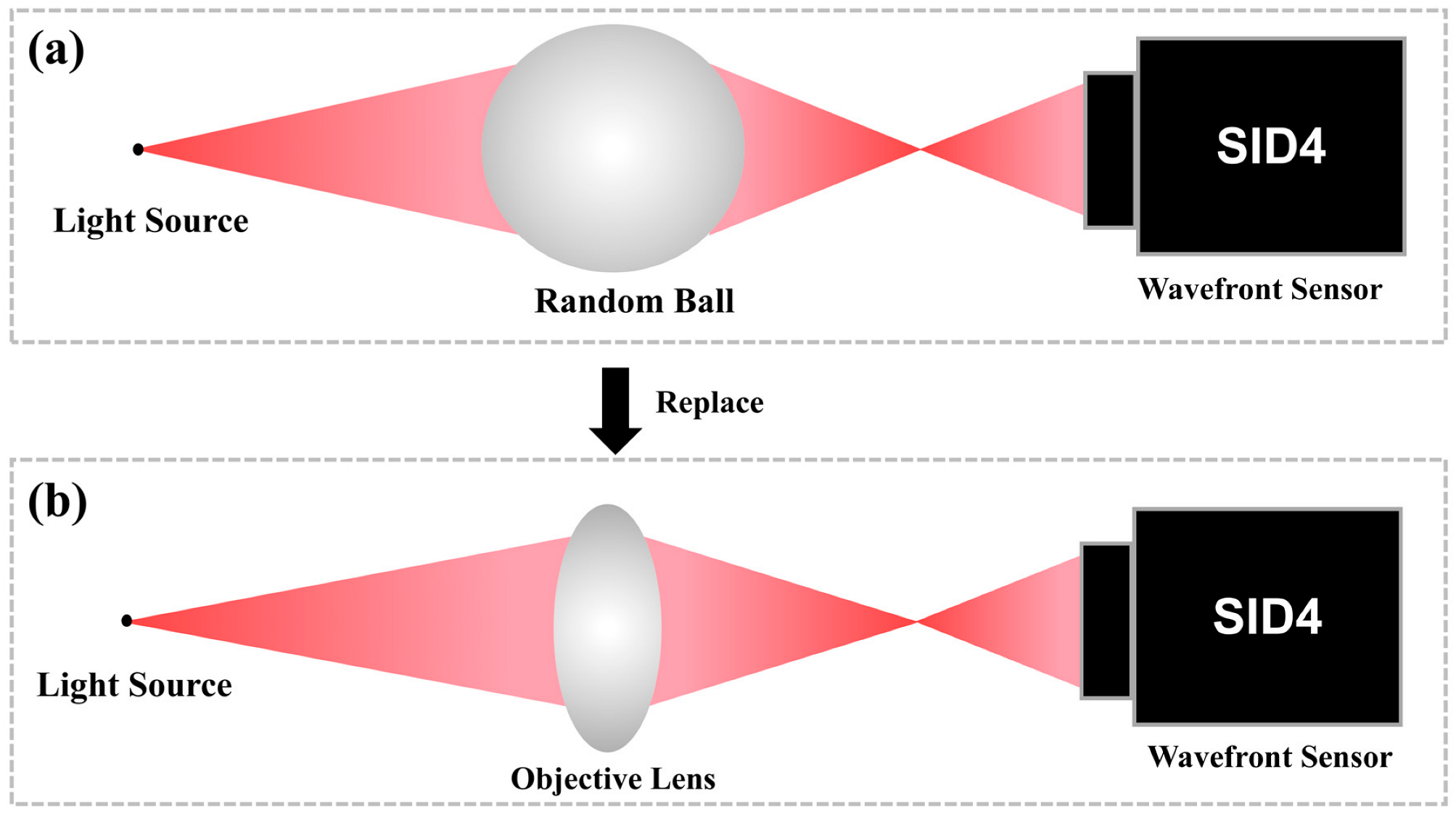
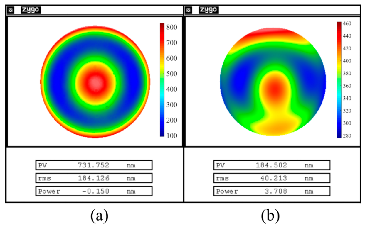
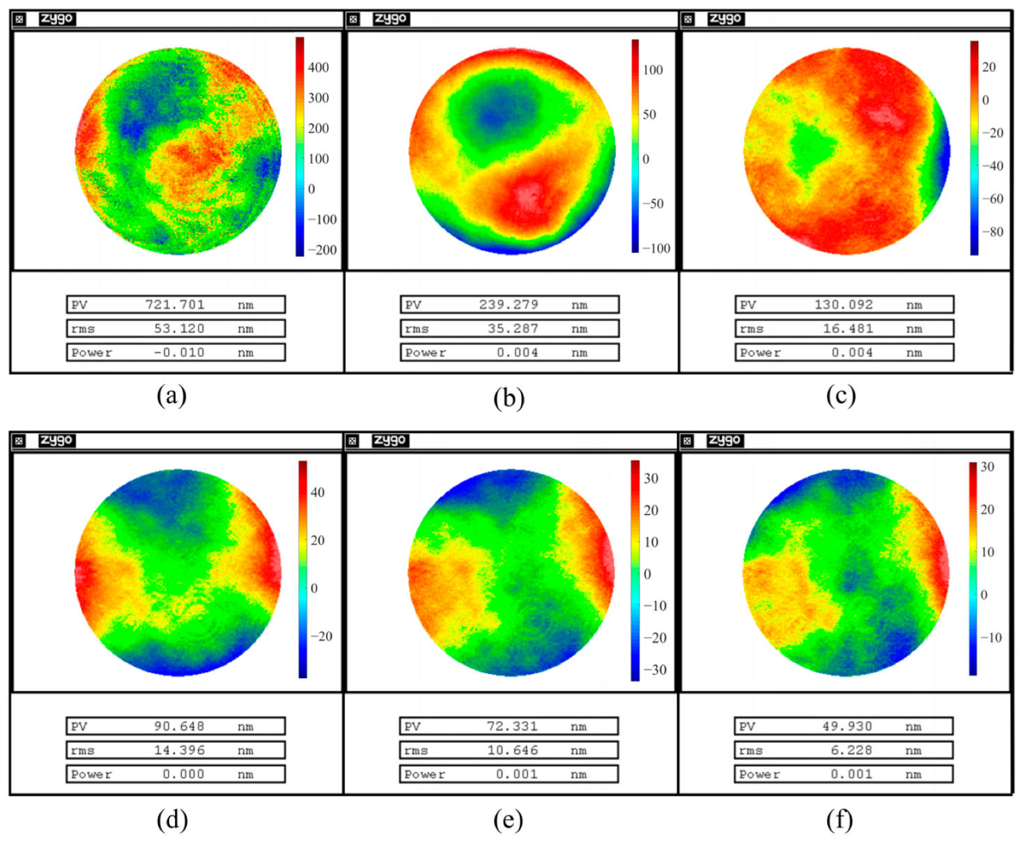
3.1. Random Ball Test
3.2. Single-Channel Measurement of the Lens
3.3. Dual-Channel Measurement of the Lens
4. Experimental Results and Discussion
4.1. NA Error Model
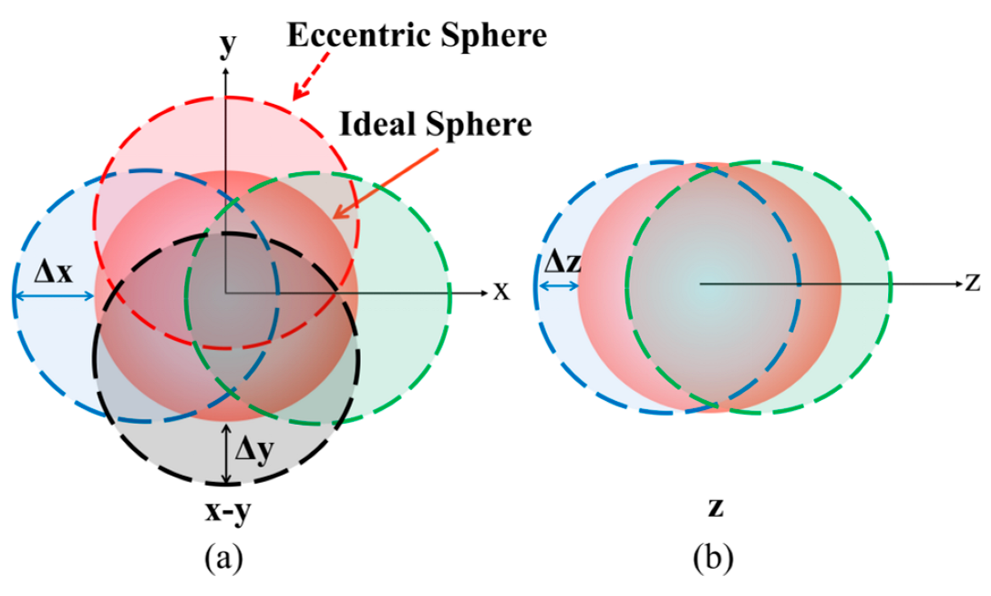
4.2. Eccentricity Model
4.3. Uncertainty Analysis
4.4. Discussion
5. Conclusions
Author Contributions
Funding
Institutional Review Board Statement
Informed Consent Statement
Data Availability Statement
Acknowledgments
Conflicts of Interest
References
- Wu, F.B.; Tang, F.; Wang, X.C.; Li, J.; Li, S.K. Research on Ronchi Shearing Interference Wavefront Aberration Detection Technology for Photolithography Projection Objectives. Chin. J. Lasers 2015, 42, 291–298. [Google Scholar]
- Cao, Y.S.; Tang, F.; Wang, X.C.; Liu, Y.; Feng, P.; Lu, Y.J.; Guo, F.D. Distortion Detection Technology for Photolithography Projection Objectives. Laser Optoelectron. Prog. 2022, 59, 216–232. [Google Scholar]
- Liu, Z.X.; Xing, T.W.; Jiang, Y.D.; Lü, B.B. Measurement of Wavefront Aberrations and Special Problems of Large Numerical Aperture Objectives. Opt. Precision Eng. 2016, 24, 482–490. [Google Scholar]
- Naulleau, P.P.; Goldberg, K.A.; Lee, S.H.; Chang, C.-H.C.; Bresloff, C.J.; Batson, P.J.; Attwood, D.T., Jr.; Bokor, J. Characterization of the accuracy of EUV phase-shifting point diffraction interferometry. In Emerging Lithographic Technologies II; SPIE: Clergy, France, 1998. [Google Scholar] [CrossRef]
- Mercère, P.; Zeitoun, P.; Idir, M.; Le Pape, S.; Douillet, D.; Levecq, X.; Dovillaire, G.; Bucourt, S.; Goldberg, K.A.; Naulleau, P.P.; et al. Hartmann wave-front measurement at 13.4 nm with λEUV/120 accuracy. Opt. Lett. 2003, 28, 1534–1536. [Google Scholar] [CrossRef]
- Miyakawa, R.; Naulleau, P. Extending shearing interferometry to high-NA for EUV optical testing. Proc. SPIE-Int. Soc. Opt. Eng. 2015, 9422, 496–501. [Google Scholar]
- Miyakawa, R.; Naulleau, P. Lateral shearing interferometry for high-resolution EUV optical testing. In Extreme Ultraviolet (EUV) Lithography II; SPIE: Clergy, France, 2011. [Google Scholar] [CrossRef]
- Dubra, A.; Paterson, C.; Dainty, C. Double lateral shearing interferometer for the quantitative measurement of tear film topography. Appl. Opt. 2005, 44, 1191–1199. [Google Scholar] [CrossRef]
- Ray-Chaudhuri, A.K.; Krenz, K.D.; Nissen, R.P.; Haney, S.J.; Fields, C.H.; Sweatt, W.C.; MacDowell, A.A. Initial results from an extreme ultraviolet interferometer operating with a compact laser plasma source. J. Vac. Sci. Technol. B 1996, 14, 3964–3968. [Google Scholar] [CrossRef]
- Ray-Chaudhuri, A.K. At-wavelength characterization of an extreme ultraviolet camera from low to mid-spatial frequencies with a compact laser plasma source. J. Vac. Sci. Technol. B Microelectron. Nanometer Struct. 1997, 15, 2462–2466. [Google Scholar] [CrossRef]
- Nikitin, A.N.; Galaktionov, I.; Sheldakova, J.; Kudryashov, A.; Baryshnikov, N.; Denisov, D.; Karasik, V.; Sakharov, A. Absolute calibration of a Shack-Hartmann wavefront sensor for measurements of wavefronts. In Photonic Instrumentation Engineering VI; SPIE: Clergy, France, 7 March 2019; 109250K. [Google Scholar] [CrossRef]
- Leith, E.N.; Hoover, B.G.; Dilworth, D.S.; Naulleau, P. Ensemble-Averaged Shack–Hartmann Wave-Front Sensing for Imaging Through Turbid Media. Appl. Opt. 1998, 37, 3643–3650. [Google Scholar] [CrossRef]
- Tao, X.; Dean, Z.; Chien, C.; Azucena, O.; Bodington, D.; Kubby, J. Shack-Hartmann wavefront sensing using interferometric focusing of light onto guide-stars. Opt. Express 2013, 21, 31282–31292. [Google Scholar] [CrossRef]
- Shahidi, M.; Yang, Y. Measurements of ocular aberrations and light scatter in healthy subjects. Optom. Vis. Sci. 2004, 81, 853–857. [Google Scholar] [CrossRef] [PubMed]
- Perez, G.M.; Manzanera, S.; Artal, P. Impact of scattering and spherical aberration in contrast sensitivity. J. Vis. 2009, 9, 19. [Google Scholar] [CrossRef] [PubMed]
- Shuang, L.; Junyan, Y.; Qingjie, S.; Chengping, L.; Xiaoning, T.; Qilong, Y.; Dai, C. Demonstration of Wavefront Measurement Technology with High-Precision and Large-Field-of-View Based on Focal Plane Hartmann Wavefront Sensor. Flight Control. Detect. 2022, 5, 12–19. [Google Scholar]
- Aihua, P.; Hongwei, Y.; Xinyang, L. Effect of Aperture Distribution on Wavefront Recovery of Lateral Shearing Interferometer. Acta Opt. Sin. 2011, 31, 15–20. [Google Scholar]
- Guo, X.; Liao, Z.; Wang, C.; Fu, R. Analysis of Vibration Effect to Surface Figure Measurement. Infrared Laser Eng. 2012, 41, 6. [Google Scholar] [CrossRef]
- Wang, R.; Tian, W.; Wang, P.; Wang, L.; Sui, Y.; Yang, H. Effect of Temperature Change on the Surface Accuracy of Bonded Lens. Chin. J. Lasers 2011, 38, 6. [Google Scholar] [CrossRef]
- Wang, R.; Tian, W.; Wang, P.; Wang, L. Analysis of Vibration Effect to Surface Figure Measurement. Acta Opt. Sin. 2012, 32, 105–108. Available online: http://ir.ciomp.ac.cn/handle/181722/28252 (accessed on 15 August 2023).
- Zhang, D.F.; Li, X.L.; Dong, L.J.; Sun, Z. Coupling Error Inhibition of Eccentric Adjustment Mechanism Design in Lithographic Objective Lens. Acta Photonica Sin. 2015, 44, 29–33. [Google Scholar] [CrossRef]
- Parks, R.E.; Evans, C.; Shao, L. Calibration of Interferometer Transmission Spheres. In Optical Fabrication and Testing, Technical Digest Series; paper OTuC.1; Optica Publishing Group: Washington, DC, USA, 1998. [Google Scholar]
- Ping, Z.; Burge, J.H. Limits for interferometer calibration using the random ball test. In Optical Manufacturing and Testing VIII; International Society for Optics and Photonics: Clergy, France, 2009. [Google Scholar]
- Burke, J.; Wu, D.S. Calibration of spherical reference surfaces for Fizeau interferometry: A comparative study of methods. Appl. Opt. 2010, 49, 6014–6023. [Google Scholar] [CrossRef]
- Zhou, P. Error Analysis and Data Reduction for Interferometric Surface Measurements. Ph.D. Dissertation, University of Arizona, Tucson, AZ, USA, 2009. [Google Scholar]
- Griesmann, U.; Wang, Q.; Soons, J.; Carakos, R. A simple ball averager for reference sphere calibrations. In Optical Manufacturing and Testing VI; SPIE: Clergy, France, 19 August 2005; p. 58690S. [Google Scholar] [CrossRef]
- Xi, H.; Shuai, Z.; Xiaochuan, H.; Haiyang, Q.; Gaofeng, W.; Xin, J.; Yiwei, H.; Qiang, C.; Fan, W. The research progress of surface interferometric measurement with higher accuracy. Opto-Electron. Eng. 2020, 47, 13. [Google Scholar] [CrossRef]
- Soons, J.A.; Griesmann, U. Absolute interferometric tests of spherical surfaces based on rotational and translational shears. Proc. SPIE-Int. Soc. Opt. Eng. 2012, 8493, 447–454. [Google Scholar] [CrossRef]
- Zhou, Y.; Ghim, Y.S.; Davies, A. Self calibration for slope-dependent errors in optical profilometry by using the random ball test. Proc. SPIE-Int. Soc. Opt. Eng. 2012, 8493, 729–740. [Google Scholar] [CrossRef]
- Defu, Z.; Xianling, L. Effect of Adjusting Force on Surface Figure of Lens in Eccentric Adjusting Mechanism. Chin. J. Lasers 2014, 41, 285–292. [Google Scholar] [CrossRef]
- Karunasingha, D.S.K. Root mean square error or mean absolute error? Use their ratio as well. Inf. Sci. 2022, 585, 609–629. [Google Scholar] [CrossRef]
- Yang, P.; Xu, J.; Zhu, J.; Hippler, S. Transmission sphere calibration and its current limits. Proc. SPIE-Int. Soc. Opt. Eng. 2011, 8082, 794–801. [Google Scholar] [CrossRef]


| Distance | Radius | Material | RAID | |
|---|---|---|---|---|
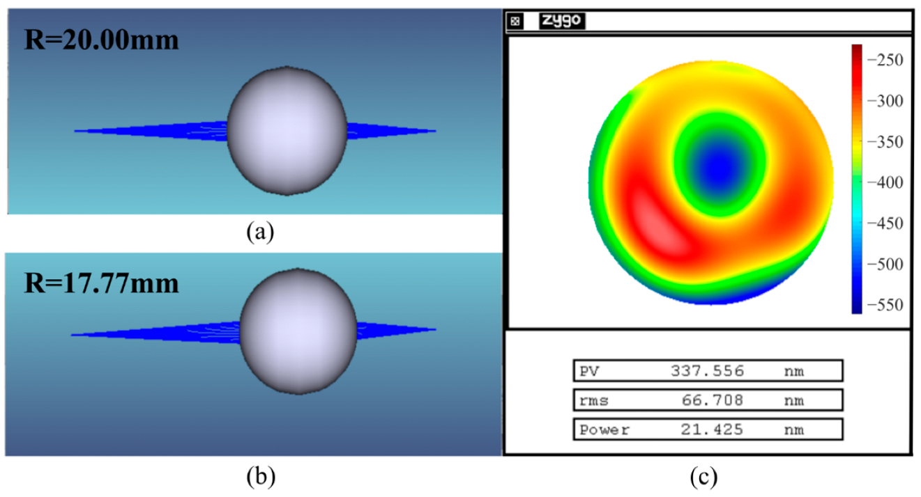
| Ideal | 50 mm | 17.77 | N-BK7 | 5.626° |
| Actual | 50 mm | 20.00 | N-BK7 | 4.856° |
| X/mm | Y/mm | Z/mm | Z5 | Z6 | Z7 | Z8 | Z9 | |
|---|---|---|---|---|---|---|---|---|
| Ideal | 0 | 0 | 0 | 0 | 0 | 0 | 0 | 0.5820 |
| Target | - | - | - | −0.0510 | −0.0250 | −0.0830 | −0.1510 | 0.7490 |
| Result | 0.053 | 0.114 | 5.242 | −0.0049 | 0.0058 | −0.0727 | −0.1573 | 0.7499 |
| △W | - | - | - | −0.0049 | 0.0058 | −0.0727 | −0.1573 | 0.1679 |
Disclaimer/Publisher’s Note: The statements, opinions and data contained in all publications are solely those of the individual author(s) and contributor(s) and not of MDPI and/or the editor(s). MDPI and/or the editor(s) disclaim responsibility for any injury to people or property resulting from any ideas, methods, instructions or products referred to in the content. |
© 2023 by the authors. Licensee MDPI, Basel, Switzerland. This article is an open access article distributed under the terms and conditions of the Creative Commons Attribution (CC BY) license (https://creativecommons.org/licenses/by/4.0/).
Share and Cite
Li, J.; Quan, H.; Jin, C.; Liu, J.; Zhu, X.; Wang, J.; Hu, S. A Model-Based Approach for Measuring Wavefront Aberrations Using Random Ball Residual Compensation. Photonics 2023, 10, 1083. https://doi.org/10.3390/photonics10101083
Li J, Quan H, Jin C, Liu J, Zhu X, Wang J, Hu S. A Model-Based Approach for Measuring Wavefront Aberrations Using Random Ball Residual Compensation. Photonics. 2023; 10(10):1083. https://doi.org/10.3390/photonics10101083
Chicago/Turabian StyleLi, Jianke, Haiyang Quan, Chuan Jin, Junbo Liu, Xianchang Zhu, Jian Wang, and Song Hu. 2023. "A Model-Based Approach for Measuring Wavefront Aberrations Using Random Ball Residual Compensation" Photonics 10, no. 10: 1083. https://doi.org/10.3390/photonics10101083
APA StyleLi, J., Quan, H., Jin, C., Liu, J., Zhu, X., Wang, J., & Hu, S. (2023). A Model-Based Approach for Measuring Wavefront Aberrations Using Random Ball Residual Compensation. Photonics, 10(10), 1083. https://doi.org/10.3390/photonics10101083