Simulated LCSLM with Inducible Diffractive Theory to Display Super-Gaussian Arrays Applying the Transport-of-Intensity Equation

 , , , ,
Abstract
1. Introduction
2. LCD Design and Construction
LCD Validation
3. TIE as an Optical Test
4. Setups
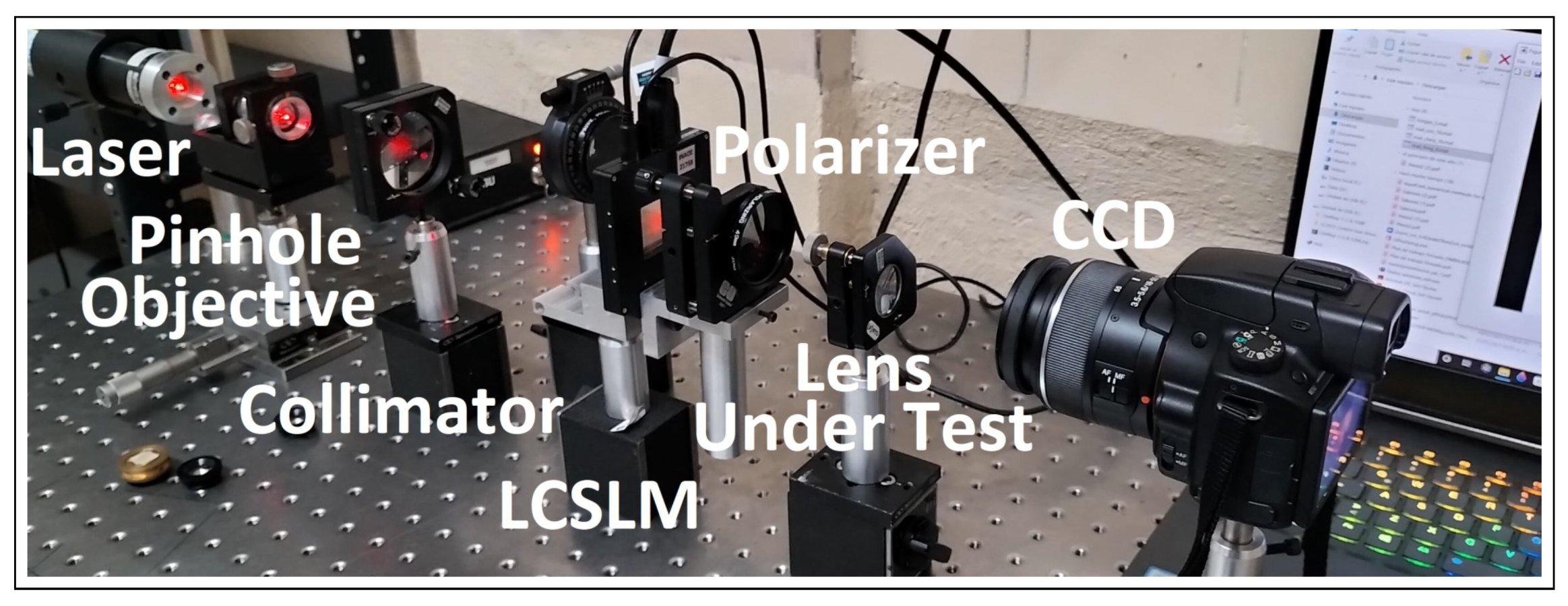
4.1. Experimental
4.2. Simulations
5. Early Results
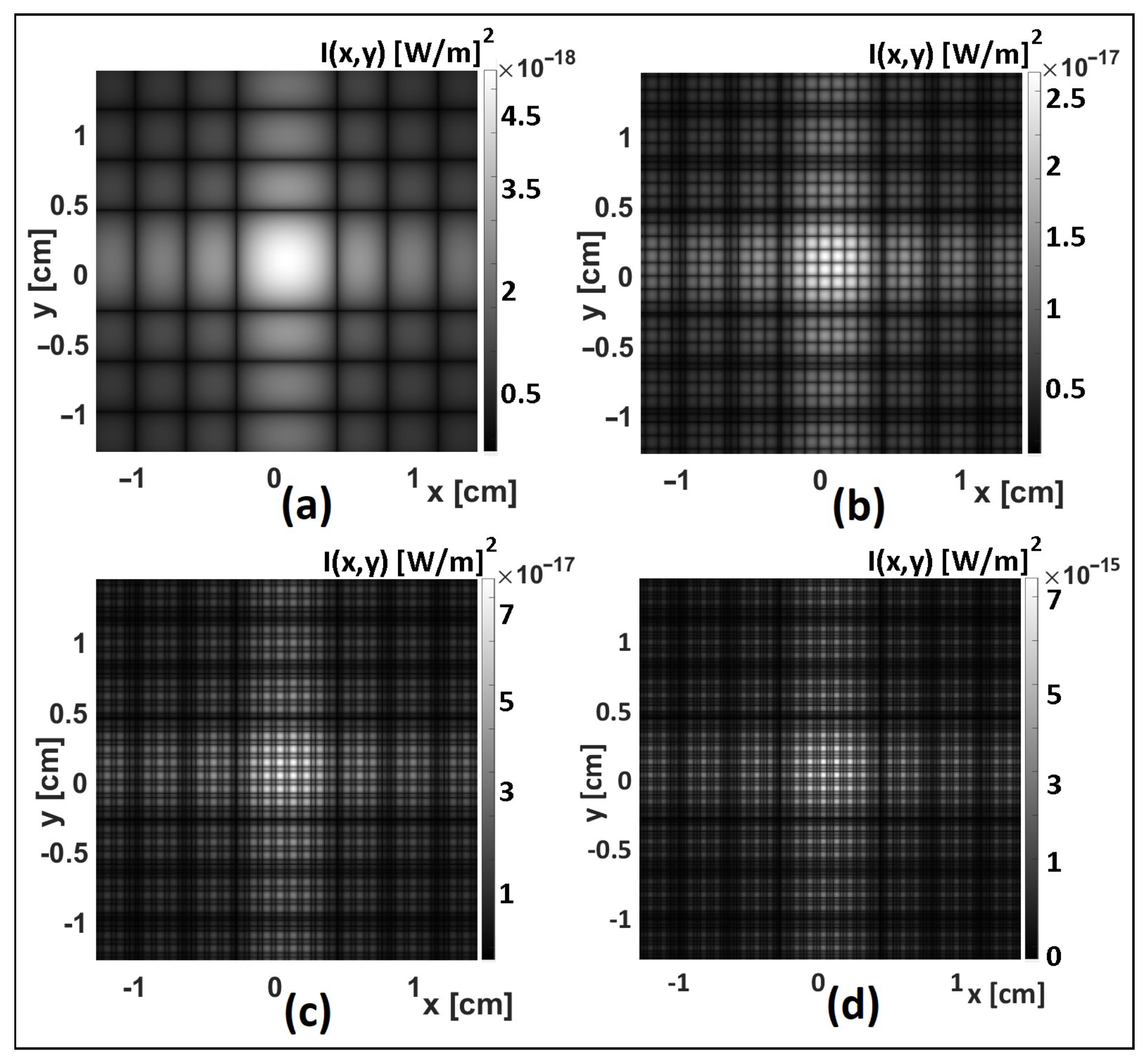
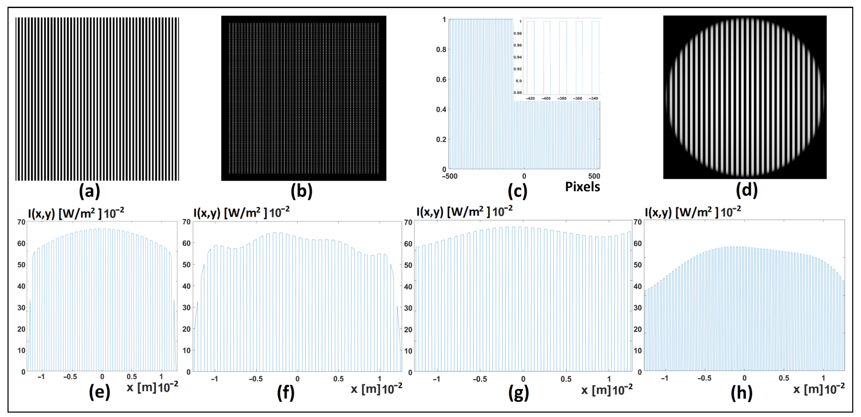
5.1. Diffraction Patterns
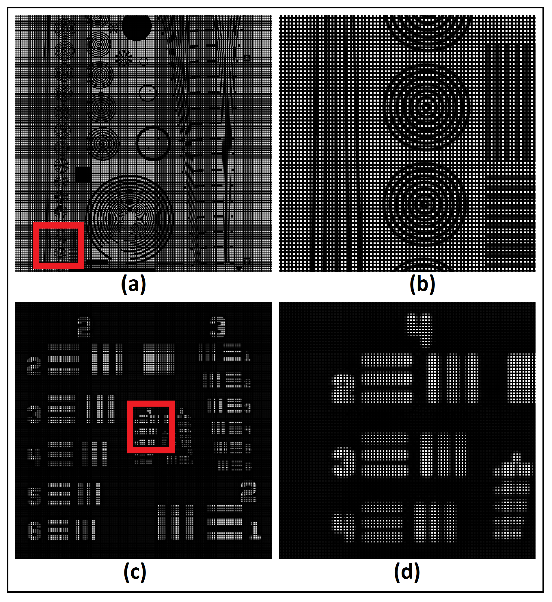
5.2. Validating the LCSLM
5.3. Super-Gaussian Profiles
6. Experimental Results
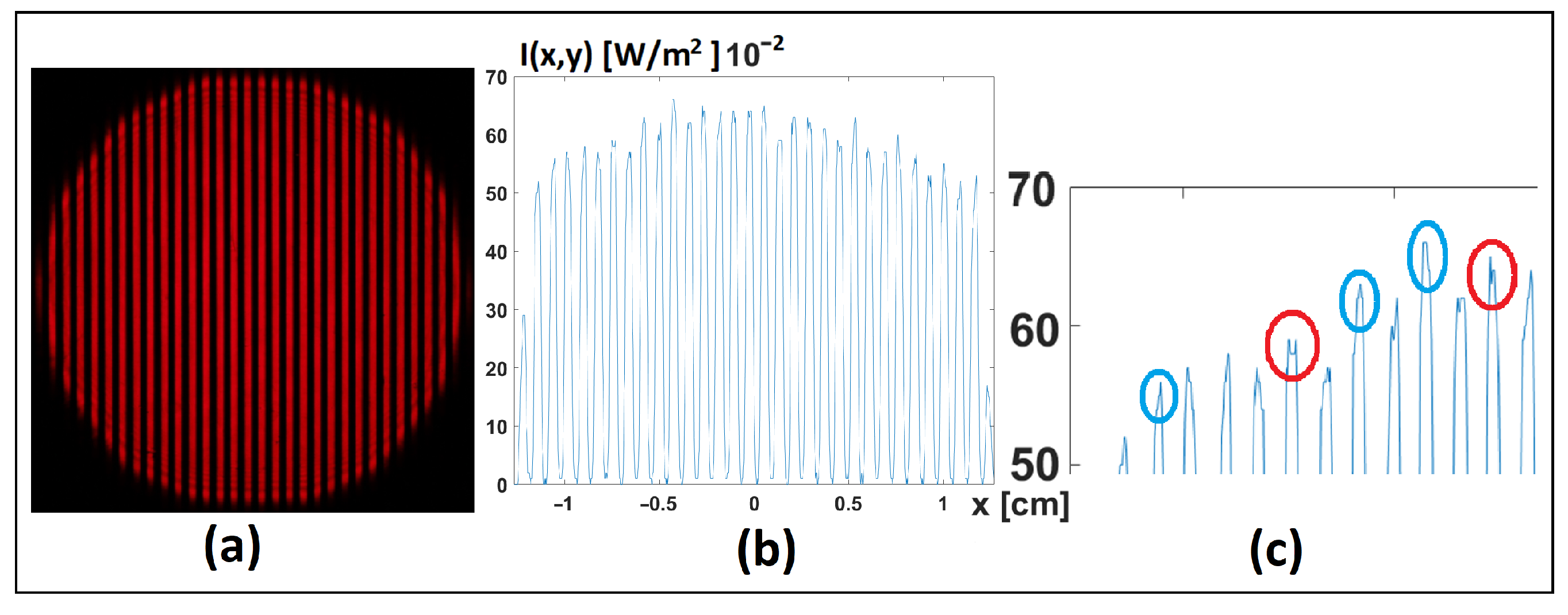
6.1. Fringes Error Reduction
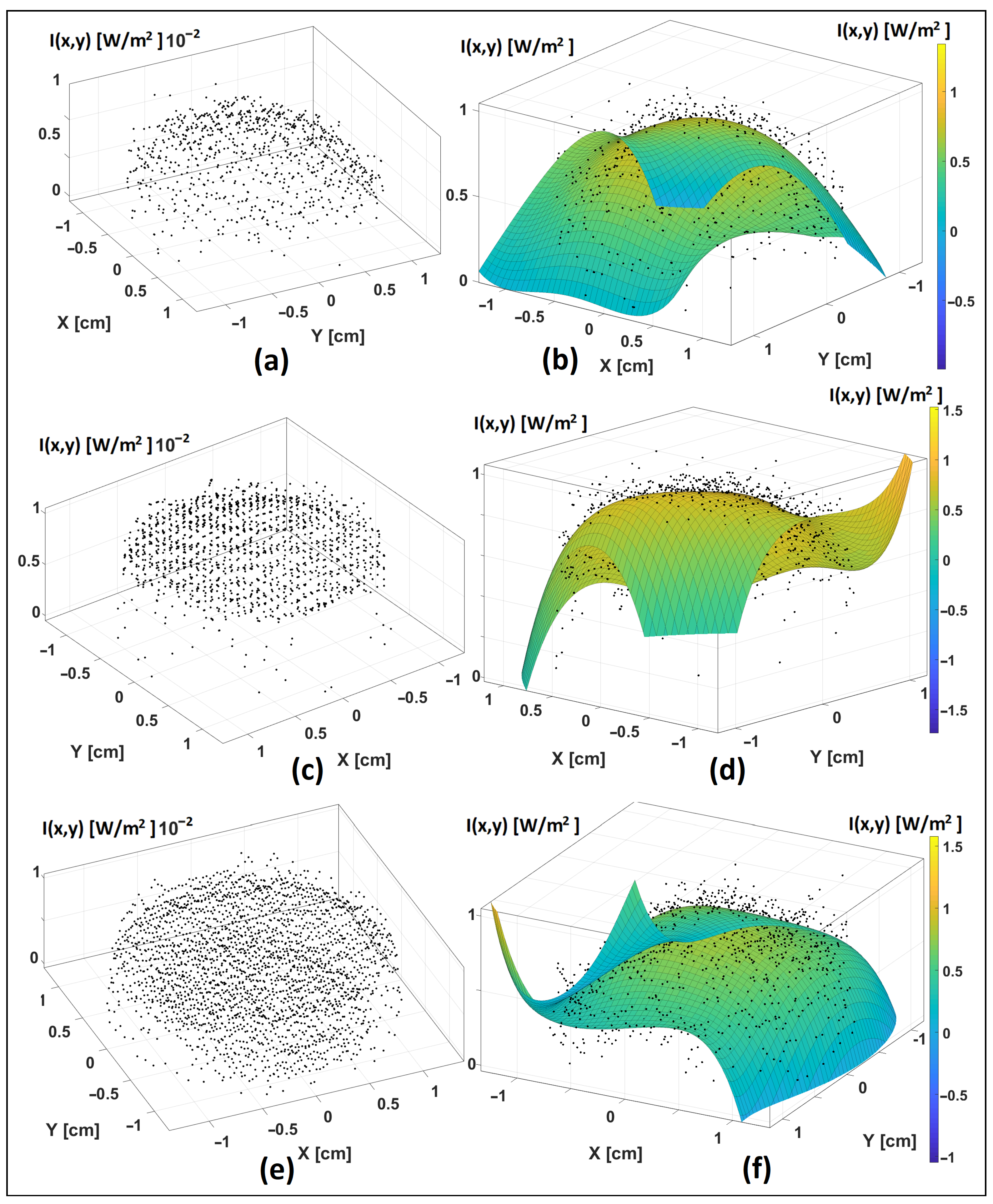
6.2. Intensity Captures
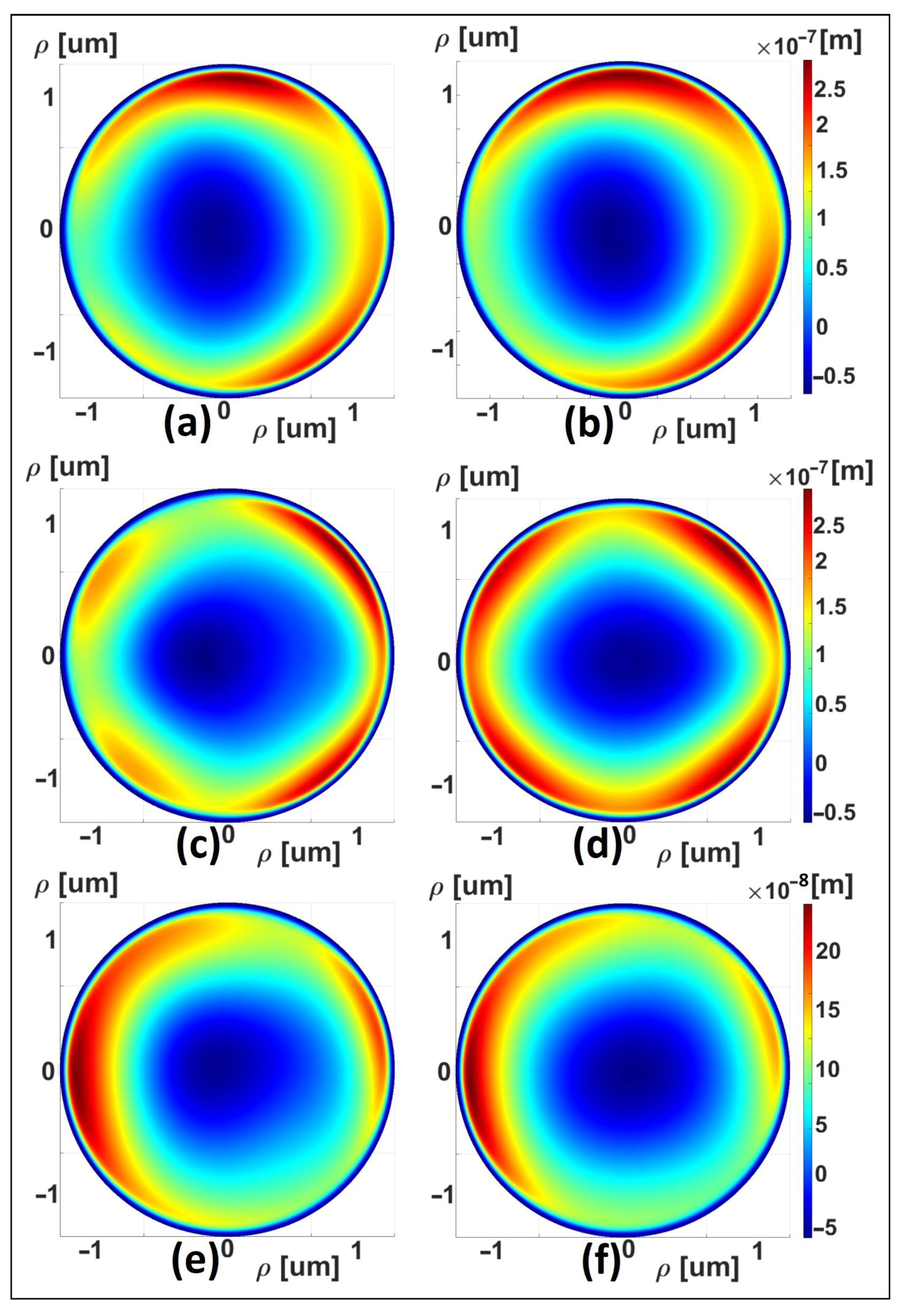
6.3. Obtaining the Wavefront
7. Conclusions
Supplementary Materials
Author Contributions
Funding
Institutional Review Board Statement
Informed Consent Statement
Data Availability Statement
Acknowledgments
Conflicts of Interest
References
- Hornbeck, L.J. Digital light processing for high-brightness high-resolution applications. In Proceedings of the Projection Displays III, Electronic Imaging ’97, San Jose, CA, USA, 8 May 1997; Volume 3013, pp. 27–40. [Google Scholar] [CrossRef]
- Zhang, T.; Kho, A.M.; Srinivasan, V.J. Improving visible light OCT of the human retina with rapid spectral shaping and axial tracking. Biomed. Opt. Express 2019, 6, 2918–2931. [Google Scholar] [CrossRef] [PubMed]
- Matsumoto, N.; Inoue, T.; Matsumoto, A.; Okazaki, S. Correction of depth-induced spherical aberration for deep observation using two-photon excitation fluorescence microscopy with spatial light modulator. Biomed. Opt. Express 2015, 6, 2575–2587. [Google Scholar] [CrossRef] [PubMed]
- Khan, S.; Jesacher, A.; Nussbaumer, W.; Bernet, S.; Ritsch-Marte, M. Quantitative analysis of shape and volume changes in activated thrombocytes in real time by single-shot spatial light modulator-based differential interference contrast imaging. J. Biophotonics 2011, 4, 600–609. [Google Scholar] [CrossRef] [PubMed]
- Ibrahim, D.G.A.; Bakr, R.H. Viewing label-free white blood cells using phase-only spatial light modulator. In Frontiers in Optics + Laser Science; Mazzali, C., Poon, T.(T.-C.), Averitt, R., Kaindl, R., Eds.; Technical Digest Series, Paper JW7A.123; Optica Publishing Group: Washington DC, WA, USA, 2021. [Google Scholar] [CrossRef]
- Ibrahim, D.G.A.; Abdelazeem, R.M. Quantitative Phase Imaging by Automatic Phase Shifting Generated by Phase-only Spatial Light Modulator. In Frontiers in Optics + Laser Science; Mazzali, C., Poon, T.(T.-C.), Averitt, R., Kaindl, R., Eds.; Technical Digest Series Paper JTh5A.104; Optica Publishing Group: Washington DC, WA, USA, 2021. [Google Scholar] [CrossRef]
- Wen, S.; Bhaskar, A.; Zhang, H. Scanning digital lithography providing high speed large area patterning with diffraction limited sub-micron resolution. J. Micromech. Microeng. 2018, 28, 075011. [Google Scholar] [CrossRef]
- Kagalwala, K.H.; Di-Giuseppe, G.; Abouraddy, A.F.; Saleh, B. Single-photon three-qubit quantum logic using spatial light modulators. Nat. Comm. 2017, 8, 739. [Google Scholar] [CrossRef]
- Storrs, M.; Mehrl, D.J.; Walkup, J.F.; Krile, T.F. Volterra series modeling of spatial light modulators. Appl. Opt. 1998, 37, 7472–7481. [Google Scholar] [CrossRef]
- Slinger, C.; Cameron, C.; Stanley, M. Computer-generated holography as a generic display technology. Computer 2005, 38, 46–53. [Google Scholar] [CrossRef]
- Chandra, A.D.; Karmakar, M.; Nandy, D.; Banerjee, A. Adaptive hyperspectral imaging using structured illumination in a spatial light modulator-based interferometer. Opt. Express 2022, 30, 19930–19943. [Google Scholar] [CrossRef]
- Hara, T. A liquid crystal spatial light phase modulator and its applications. In Information Optics and Photonics Technology, Proceedings of the Photonics Asia, Beijing, China, 11 January 2005; SPIE: Bellingham, WA, USA, 2004; Volume 5642, pp. 78–89. [Google Scholar] [CrossRef]
- Chandra, A.D.; Banerjee, A. Rapid phase calibration of a spatial light modulator using novel phase masks and optimization of its efficiency using an iterative algorithm. J. Modern Opt. 2020, 67, 628–637. [Google Scholar] [CrossRef]
- Davis, J.A.; Tsai, P.S.; Cottrell, D.M.; Sonehara, T.; Amako, J.; Santillan, A. Transmission variations in liquid crystal spatial light modulators caused by interference and diffraction effects. Opt. Eng. 1999, 38, 1051–1057. [Google Scholar] [CrossRef]
- Pérez-Cabré, E.; Millán-Sagrario, M. Liquid Crystal Spatial Light Modulator with Optimized Phase Modulation Ranges to Display Multiorder Diffractive Elements. App. Sci. 2019, 9, 2592. [Google Scholar] [CrossRef]
- Katz, B.; Rosen, J.; Kelner, R.; Brooker, G. Enhanced resolution and throughput of Fresnel incoherent correlation holography (FINCH) using dual diffractive lenses on a spatial light modulator (SLM). Opt. Express 2012, 20, 9109–9121. [Google Scholar] [CrossRef] [PubMed]
- Agour, M.; Kolenovic, E.; Falldorf, C.; von-Kopylow, C. Suppression of higher diffraction orders and intensity improvement of optically reconstructed holograms from a spatial light modulator. J. Opt. 2009, 11, 105405. [Google Scholar] [CrossRef]
- Frantz, M. A Fractal Made of Golden Sets. Math. Mag. 2009, 82, 243–254. Available online: https://www.jstor.org/stable/27765915 (accessed on 24 December 2022). [CrossRef]
- Horváth, P.; Šmíd, P.; Vašková, I.; Hrabovský, M. Koch fractals in physical optics and their Fraunhofer diffraction patterns. Optik 2010, 121, 206–213. [Google Scholar] [CrossRef]
- Wang, J.; Zhang, W.; Cui, Y.; Teng, S. Fresnel diffraction of fractal grating and self-imaging effect. Appl. Opt. 2014, 53, 2105–2111. [Google Scholar] [CrossRef]
- Henkin, L. On Mathematical Induction. Am. Math. Mon. 1960, 67, 323–338. [Google Scholar] [CrossRef]
- Arriaga-Hernández, J.A.; Granados-Agustín, F.; Cornejo-Rodríguez, A. Measurement of three-dimensional wavefronts using the Ichikawa-Lohmann-Takeda solution to the irradiance transport equation. Appl. Opt. 2018, 57, 4316–4321. [Google Scholar] [CrossRef]
- Ichikawa, K.; Lohmann, A.W.; Takeda, M. Phase retrieval based on the irradiance transport equation and the Fourier transform method: Experiments. Appl. Opt. 1988, 27, 3433–3436. [Google Scholar] [CrossRef]
- Vasudevan, L.; Fleck, A. Zernike polynomials: A guide. J. Mod. Opt. 2011, 58, 545–561. [Google Scholar] [CrossRef]
- von-Zernike, F. Beugungstheorie des schneidenver-fahrens und seiner verbesserten form, der phasenkontrastmethode. Physica 1934, 1, 689–704. [Google Scholar] [CrossRef]
- Arriaga, J.A.; Cuevas, B.T.; Oliveros, J.J.; Jaramillo, A.; Morín, M. Irradiance transport equation applied to propagation of wavefront obtained by the Bi-Ronchi test using point cloud. J. Phys. Commun. 2021, 5, 055019. [Google Scholar] [CrossRef]
- Forman, P.F. Digital light processing for high-brightness high-resolution applications. In Proceedings of the 23rd Annual Technical Symposium, San Diego, CA, USA, 25 December 1979; Volume 0192, pp. 41–49. [Google Scholar] [CrossRef]
- Teague, M.R. Deterministic phase retrieval: A Green’s function solution. J. Opt. Soc. Am. 1983, 73, 1434–1441. [Google Scholar] [CrossRef]
- Mohamed, N. Digital Filters Design for Signal and Image; Wiley-ISTE: Newport Beach, CA, USA, 2008. [Google Scholar] [CrossRef]
- Pratt, W.K. Digital Image Processing; John Wiley & Sons: Los Altos, CA, USA, 2002. [Google Scholar] [CrossRef]
- Vetterli, M.; Kovačević, J.; Goyal, V.K. Foundations of Signal Processing; Cambridge University Press: Cambridge, UK, 2014. [Google Scholar] [CrossRef]
- Arendt, W.; Schleich, W.P. Mathematical Analysis of Evolution, Information, and Complexity; Wiley-VCH Verlag GmbH & Co. KGaA: Weinheim, Germany, 2009. [Google Scholar] [CrossRef]
- Mandel, L.; Wolf, E. Optical Coherence and Quantum Optics; Cambridge University Press: Rochester, NY, USA, 1995. [Google Scholar] [CrossRef]
- Born, M.; Wolf, E. Principles of Optics: Electromagnetic Theory of Propagation, Interference and Diffraction of Light; Cambridge University Press: Cambridge, UK, 2000. [Google Scholar] [CrossRef]
- Goodman, J.W. Introduction to Fourier Optics; E W. H. Freeman Press: San Francisco, CA, USA, 2005. [Google Scholar] [CrossRef]
- Roe, E.D. Note on Integral and Integro-Geometric Series. Ann. Math. 1896, 11, 184–194. [Google Scholar] [CrossRef]
- Arfken, G.B.; Weber, H.J.; Harris, F. Mathematical Methods for Physicists; Elsevier Academic Press: London, UK, 2012. [Google Scholar] [CrossRef]
- Hirst, K. Numbers, Sequences and Series; Elsevier Academic Press: Southampton, UK, 1994. [Google Scholar]
- Dorrer, C.; Zuegel, J.D. Optical testing using the transport-of-intensity equation. Opt. Express 2007, 15, 7165–7175. [Google Scholar] [CrossRef]
- Gupta, A.K.; Mahendra, R.; Nishcal, K.N. Single-shot phase imaging based on transport of intensity equation. Opt. Comm. 2020, 477, 126347. [Google Scholar] [CrossRef]
- Kovalev, M.; Gritsenko, I.; Stsepuro, N.; Nosov, P.; Krasin, G.; Kudryashov, S. Reconstructing the Spatial Parameters of a Laser Beam Using the Transport-of-Intensity Equation. Sensors 2022, 5, 1765. [Google Scholar] [CrossRef]
- Verdeyen, J.T. Laser Electronics; Prentice Hall Press: Urbana, IL, USA, 1995. [Google Scholar]
- Ronchi, V. Due nuovi metodi per lo studio delle superficie e dei sistemi ottici. In Annali della Scuola Normale Superiore di Pisa–Classe di Scienze; Springer Nature: Berlin/Heidelberg, Germany, 1927; Volume 69, pp. 69–71. [Google Scholar] [CrossRef]
- Bergeron, A.; Gauvin, J.; Gagnon, F.; Gingras, D.; Arsenault, H.H.; Doucet, M. Phase calibration and applications of a liquid-crystal spatial light modulator. Appl. Opt. 1995, 34, 5133–5139. [Google Scholar] [CrossRef]
- Shetty, P.P.; Bingi, J. Demonstration of synergic Fresnel and Fraunhofer diffraction for application to micrograting fabrication. Opt. Laser Technol. 2020, 130, 106340. [Google Scholar] [CrossRef]
- Zhou, J.; Cao, Z.; Xie, H.; Xu, L. Digital micro-mirror device-based detector for particle-sizing instruments via Fraunhofer diffraction. Appl. Opt. 2015, 54, 5842–5849. [Google Scholar] [CrossRef]
- Malacara, D. Optical Shop Testing; John Wiley & Sons Inc.: Hoboken, NJ, USA, 2007. [Google Scholar] [CrossRef]
- Bissell, J.J.; Ridgers, C.P.; Kingham, R.J. Super-Gaussian transport theory and the field-generating thermal instability in laser–plasmas. New J. Phys. 2013, 15, 025017. [Google Scholar] [CrossRef]
- De-Silvestri, S.; Laporta, P.; Magni, V.; Svelto, O. Solid-state laser unstable resonators with tapered reflectivity mirrors: The super-Gaussian approach. J. Quantum Electron. 1988, 24, 1172–1177. [Google Scholar] [CrossRef]
- Arriaga, J.A.; Cuevas, B.T.; Oliveros, J.J.; Jaramillo, A.; Morín, M. Filter construction using Ronchi masks and Legendre polynomials to analyze the noise in aberrations by applying the irradiance transport equation. Appl. Opt. 2020, 59, 3851–3860. [Google Scholar] [CrossRef] [PubMed]
- Glowinski, R.; Neittaanmäki, P. Partial Differential Equations: Modelling and Numerical Simulation. In Computational Methods in Applied Sciences; Springer: Dordrecht, The Netherlands, 2008. [Google Scholar] [CrossRef]
- Glowinski, R. Finite element methods for incompressible viscous flow. In Handbook of Numerical Analysis; Elsevier: Amsterdam, The Netherlands, 2003; Volume 9, pp. 3–1176. [Google Scholar] [CrossRef]
- Yin, P.; Liandrat, J.; Shen, W. A comparison of the finite difference and multiresolution method for the elliptic equations with Dirichlet boundary conditions on irregular domains. J. Comput. Phys. 2021, 343, 110207. [Google Scholar] [CrossRef]
- Birkes, D.; Dodge, D. Alternative Methods of Regression; John Wiley & Sons: New York, NY, USA, 1993. [Google Scholar]
- Arriaga, J.A.; Cuevas, B.T.; Oliveros, J.J.; Jaramillo, A.; Morín, M. Geometric aberrations in the 3D profile of microparticles observed in optical trapping using 2D Legendre polynomials. Optik 2022, 249, 168123. [Google Scholar] [CrossRef]


| L1 [m] × 10 | |||||
| ANSI | Coeff | Aberration | Exp RR | SGR in LCD | ZYGO/APEX |
| 1 | piston | 11.5223 | 12.4140 | 12.1610 | |
| 5 | defocus | 6.9981 | 7.3471 | 7.3831 | |
| 4 | Astig 45° | −1.4970 | −1.5073 | −1.5587 | |
| 6 | Astig 0° | −1.9338 | −2.0570 | −2.0855 | |
| 8 | coma x | −0.5006 | −0.5890 | −0.4807 | |
| 9 | coma y | −1.6599 | −1.7658 | −1.8214 | |
| 13 | Spherical | −8.9067 | −8.3279 | −8.2557 | |
| L2 [m] × 10 | |||||
| ANSI | Coeff | Aberration | Exp RR | SGR in LCD | ZYGO/APEX |
| 1 | piston | 12.9901 | 13.9450 | 13.2360 | |
| 5 | defocus | 8.2316 | 8.8043 | 9.0063 | |
| 4 | Astig 45° | 0.4003 | 0.3721 | 0.1800 | |
| 6 | Astig 0° | −0.4733 | −0.4895 | −0.5259 | |
| 8 | coma x | −0.1723 | −0.1670 | −0.1506 | |
| 9 | coma y | 1.9801 | 2.5862 | 0.5937 | |
| 13 | Spheric | −8.0072 | −8.8874 | −8.4999 | |
| L3 [m] × 10 | |||||
| ANSI | Coeff | Aberration | Exp RR | SGR in LCD | ZYGO/APEX |
| 1 | piston | 9.3109 | 9.5123 | 9.2009 | |
| 5 | defocus | 5.7501 | 5.5605 | 5.6785 | |
| 4 | Astig 45° | 1.9988 | 3.0229 | 0.2762 | |
| 6 | Astig 0° | 2.0089 | 2.1026 | 2.1489 | |
| 8 | coma x | −0.5006 | −0.4412 | −0.2752 | |
| 9 | coma y | 0.4591 | 0.4653 | 0.3170 | |
| 13 | Spherical | −6.7001 | −6.6191 | −6.4783 | |
Disclaimer/Publisher’s Note: The statements, opinions and data contained in all publications are solely those of the individual author(s) and contributor(s) and not of MDPI and/or the editor(s). MDPI and/or the editor(s) disclaim responsibility for any injury to people or property resulting from any ideas, methods, instructions or products referred to in the content. |
© 2022 by the authors. Licensee MDPI, Basel, Switzerland. This article is an open access article distributed under the terms and conditions of the Creative Commons Attribution (CC BY) license (https://creativecommons.org/licenses/by/4.0/).
Share and Cite
Arriaga-Hernandez, J.; Cuevas-Otahola, B.; Oliveros-Oliveros, J.; Morín-Castillo, M.; Martínez-Laguna, Y.; Cedillo-Ramírez, L. Simulated LCSLM with Inducible Diffractive Theory to Display Super-Gaussian Arrays Applying the Transport-of-Intensity Equation. Photonics 2023, 10, 39. https://doi.org/10.3390/photonics10010039
Arriaga-Hernandez J, Cuevas-Otahola B, Oliveros-Oliveros J, Morín-Castillo M, Martínez-Laguna Y, Cedillo-Ramírez L. Simulated LCSLM with Inducible Diffractive Theory to Display Super-Gaussian Arrays Applying the Transport-of-Intensity Equation. Photonics. 2023; 10(1):39. https://doi.org/10.3390/photonics10010039
Chicago/Turabian StyleArriaga-Hernandez, Jesus, Bolivia Cuevas-Otahola, Jacobo Oliveros-Oliveros, María Morín-Castillo, Ygnacio Martínez-Laguna, and Lilia Cedillo-Ramírez. 2023. "Simulated LCSLM with Inducible Diffractive Theory to Display Super-Gaussian Arrays Applying the Transport-of-Intensity Equation" Photonics 10, no. 1: 39. https://doi.org/10.3390/photonics10010039
APA StyleArriaga-Hernandez, J., Cuevas-Otahola, B., Oliveros-Oliveros, J., Morín-Castillo, M., Martínez-Laguna, Y., & Cedillo-Ramírez, L. (2023). Simulated LCSLM with Inducible Diffractive Theory to Display Super-Gaussian Arrays Applying the Transport-of-Intensity Equation. Photonics, 10(1), 39. https://doi.org/10.3390/photonics10010039