
A Modelling Approach for the Management of Invasive Species at a High-Altitude Artificial Lake

 ,
,  ,
, 

Abstract
:1. Introduction
2. Materials and Methods
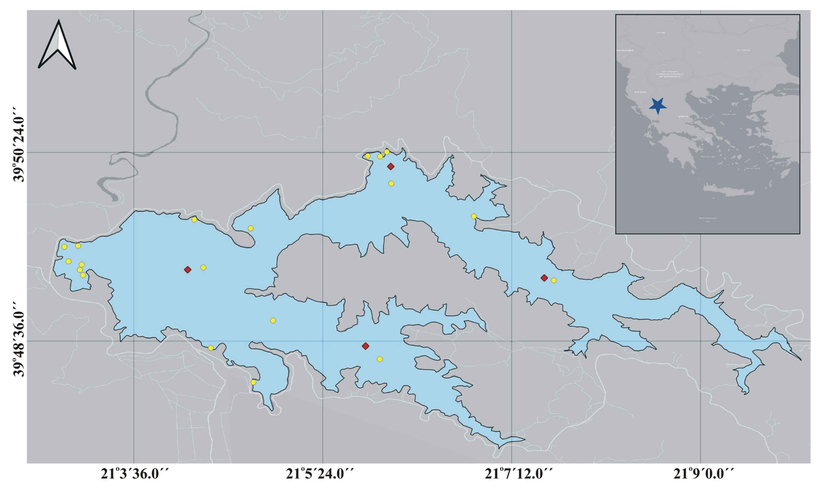
2.1. Study Area
2.2. Interview Survey
2.3. Model Parameterisation
2.4. Ecosystem Indicators and Sensitivity
3. Results
3.1. Sensitivity Analysis
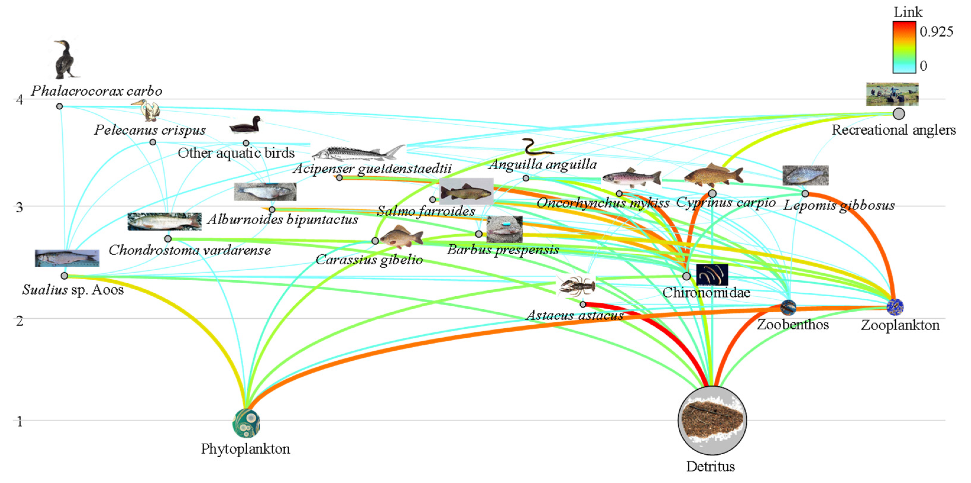
3.2. Food Web Structure
3.3. Ecosystem Approach
4. Discussion
5. Conclusions
Author Contributions
Funding
Data Availability Statement
Acknowledgments
Conflicts of Interest
Appendix A
Appendix B

| Species/Taxa Groups | Description | Reference |
|---|---|---|
| Cormorants (Phalacrocorax carbo) | ||
| B | Estimated from the records of the Management Body (N2KGR1310002) (2021–2022) | [48,49] |
| P/B | Empirical equations based on [50] | [4,51,52] |
| Q/B | Empirical equations | [4,29,51,52,53,54] |
| Diet | Diet composition | [4,51,52,53,54] |
| Pelicans (Pelecanus crispus) | ||
| B | Estimated from the records of the Management Body (N2KGR1310002) (2021–2022) | [48,49] |
| P/B | Empirical equations based on [50] | [4,51,52,55] |
| Q/B | Empirical equations | [4,51,52,55] |
| Diet | Diet composition | [4,51,52,55] |
| Other aquatic birds (Anas spp., Ardea cinerea, Aythya spp., Calidris spp., Cygnus olor, Egretta spp., Fulica atra, Gallinago gallinago, Mergus serrator, Numenius arquata, Platalea leucorodia, Pluvialis spp., Phoenicopterus ruber, Podiceps spp., Recurvirostra avocetta, Tachybaptus ruficollis, Tadorna tadorna, Tringa spp., Vanellus vanellus) | ||
| B | Estimated from the records of the Management Body (N2KGR1310002) (2021–2022) | [48,49] |
| P/B | Empirical equations based on [50] | [51,52] |
| Q/B | Empirical equations | [4,51,52,55] |
| Diet | Diet composition | [4,51,52,55] |
| Acipenser gueldenstaedtii | ||
| B | Due to the low quantities of the species biomass was estimated from the model | E = 0.99 |
| P/B | Z = F + M | [56] |
| Q/B | Empirical equations | [56,57] |
| Diet | Diet composition | [56] |
| Fisheries catches | Data reported from interviews of local shored-based recreational anglers (2021–2022) | |
| Salmo farioides | ||
| B | Due to the low quantities of the species biomass was estimated from the model | E = 0.99 |
| P/B | Z = F + M | [56] |
| Q/B | Empirical equations | [56,57] |
| Diet | Diet composition | [56] |
| Fisheries catches | Data reported from interviews of local shored-based recreational anglers (2021–2022) | |
| Anguilla anguilla | ||
| B | Due to the low quantities of the species biomass was estimated from the model | E = 0.99 |
| P/B | Empirical equations based on [50] | [56] |
| Q/B | Empirical equations | [56,57] |
| Diet | Diet composition | [58,59] |
| Fisheries catches | Data reported from interviews of local shored-based recreational anglers (2021–2022). | |
| Oncorhynchus mykiss | ||
| B | Due to the low quantities of the species biomass was estimated from the model | E = 0.99 |
| P/B | Z = F + M | [56] |
| Q/B | Empirical equations | [56,57] |
| Diet | Diet composition | [56] |
| Fisheries catches | Data reported from interviews of local shored-based recreational anglers (2021–2022) | |
| Squalius sp. Aoos | ||
| B | Estimated from seasonal samplings in the artificial lake of Aoos (2021–2022) | |
| P/B | Empirical equations based on [50] | [56] |
| Q/B | Empirical equations | [56,57] |
| Diet | Diet composition | [56] |
| Fisheries catches | Data reported from interviews of local shored-based recreational anglers (2021–2022) | |
| Chondrostoma vardarense | ||
| B | Estimated from seasonal samplings in the artificial lake of Aoos (2021–2022) | |
| P/B | Z = F + M | [56] |
| Q/B | Empirical equations | [56,57] |
| Diet | Diet composition | [56] |
| Fisheries catches | Data reported from interviews of local shored-based recreational anglers (2021–2022) | |
| Cyprinus carpio | ||
| B | Estimated from seasonal samplings in the artificial lake of Aoos (2021–2022) | |
| P/B | Z = F + M | [4,60,61] |
| Q/B | Consumption/Biomass | [4] |
| Diet | Diet composition | [58] |
| Fisheries catches | Data reported from interviews of local shored-based recreational anglers (2021–2022) | |
| Alburnoides bipunctatus | ||
| B | Estimated from seasonal samplings in the artificial lake of Aoos (2021–2022) | |
| P/B | Z = F + M | [56] |
| Q/B | Consumption/biomass | [56,57] |
| Diet | Diet composition | [56] |
| Fisheries catches | Data reported from interviews of local shored-based recreational anglers (2021–2022) | |
| Carassius gibelio | ||
| B | Estimated from seasonal samplings in the artificial lake of Aoos (2021–2022) | |
| P/B | Z = F + M | [4,62,63] |
| Q/B | Consumption/biomass | [4,59] |
| Diet | Diet composition | [58,64] |
| Fisheries catches | Data reported from interviews of local shored-based recreational anglers during (2021–2022) | |
| Barbus prespensis | ||
| B | Estimated from seasonal samplings in the artificial lake of Aoos (2021–2022) | |
| P/B | Z = F + M | [56] |
| Q/B | Consumption/biomass | [56,57] |
| Diet | Diet composition | [56] |
| Fisheries catches | Data reported from interviews of local shored-based recreational anglers (2021–2022) | |
| Lepomis gibbosus | ||
| B | Estimated from seasonal samplings in the artificial lake of Aoos (2021–2022) | |
| P/B | Z = F + M | [56] |
| Q/B | Consumption/biomass | [56,57] |
| Diet | Diet composition | [56] |
| Fisheries catches | Data reported from interviews of local shored-based recreational anglers (2021–2022) | |
| Astacus astacus | ||
| B | Due to the low quantities of the species biomass was estimated from the model | E = 0.99 |
| P/B | Z = F + M | [65] |
| Q/B | Consumption/biomass | [57,65] |
| Diet | Diet composition | [65] |
| Fisheries catches | Data reported from interviews of local shored-based recreational anglers (2021–2022) | |
| Chironomidae | ||
| B | Estimated by seasonal samplings in the artificial lake of Aoos (2021–2022) | |
| P/B | Estimated from other models | [4,66,67,68,69] |
| Q/B | Estimated from other models | [4,66,67,68,69] |
| Diet | Estimated from other models | [4,66,67,68,69] |
| Zoobenthos | ||
| B | Estimated by seasonal samplings in the artificial lake of Aoos (2021–2022) | |
| P/B | Estimated from other models | [4,66,67,68,69] |
| Q/B | Estimated from other models | [4,66,67,68,69] |
| Diet | Estimated from other models | [4,66,67,68,69] |
| Zooplankton | ||
| B | Estimated by seasonal samplings in the artificial lake of Aoos (2021–2022) | |
| P/B | Estimated by the equation Log (P/B) = −0.73 − 0.23 × log (w); w is the average dry weight (=2.132 μg/specimen) of the zooplankton groups, based on the most representative group at 90% (copepods and cladocera). CF (=1.12) is a correction factor. | [4,16,29,66,67] |
| Q/B | Estimated by other models for the most dominant group in the study area. | [4,29,66,67] |
| Diet | Taking into account that bivalves was the most representative group during winter and copepods in the rest seasons, their average contribution was used to balance the seasonal diet composition. | [4,29,66,67] |
| Phytoplankton | ||
| B | Estimated by seasonal samplings in the artificial lake of Aoos (2021–2022). Carbon to Chla ratio 40:1 was used. Biomass was estimated by the classification of Lake Trichonida based on the OECD system (1982) was used. The Euphotic Zone (EUZ) was estimated from the average seasonal value of the Secchi disk (3 × Secchi depth) and was equal to 22.5. | [4,15,29,66,67] |
| P/B | Estimated from the primary production within the day for 365 days a year. | [4,29,66,67] |
| Detritus | ||
| B | Estimated from the equation of [47]: Log D = 0.954 × LogPPR + 0.863 × LogEUZ − 2.41. The Euphotic Zone (EUZ) was estimated from the average seasonal values observed by the Secchi disk (3 × Secchi depth = 22.5). | [15] |
| Code | 1 | 2 | 3 | 4 | 5 | 6 | 7 | 8 | 9 |
|---|---|---|---|---|---|---|---|---|---|
| 1 | 0.000 | 0.000 | 0.000 | 0.000 | 0.000 | 0.000 | 0.000 | 0.000 | 0.000 |
| 2 | 0.000 | 0.000 | 0.000 | 0.000 | 0.000 | 0.000 | 0.000 | 0.000 | 0.000 |
| 3 | 0.000 | 0.000 | 0.000 | 0.000 | 0.000 | 0.000 | 0.000 | 0.000 | 0.000 |
| 4 | 0.000 | 0.000 | 0.000 | 0.000 | 0.000 | 0.000 | 0.000 | 0.000 | 0.000 |
| 5 | 0.000 | 0.000 | 0.000 | 0.000 | 0.000 | 0.000 | 0.000 | 0.000 | 0.000 |
| 6 | 0.000 | 0.000 | 0.000 | 0.000 | 0.000 | 0.000 | 0.000 | 0.000 | 0.000 |
| 7 | 0.000 | 0.000 | 0.000 | 0.000 | 0.000 | 0.000 | 0.000 | 0.000 | 0.000 |
| 8 | 0.025 | 0.100 | 0.025 | 0.000 | 0.000 | 0.000 | 0.000 | 0.000 | 0.000 |
| 9 | 0.025 | 0.050 | 0.025 | 0.000 | 0.000 | 0.000 | 0.000 | 0.025 | 0.000 |
| 10 | 0.020 | 0.000 | 0.000 | 0.000 | 0.000 | 0.000 | 0.000 | 0.000 | 0.000 |
| 11 | 0.020 | 0.025 | 0.025 | 0.000 | 0.000 | 0.000 | 0.000 | 0.025 | 0.000 |
| 12 | 0.000 | 0.000 | 0.000 | 0.000 | 0.000 | 0.000 | 0.000 | 0.050 | 0.000 |
| 13 | 0.010 | 0.005 | 0.020 | 0.000 | 0.000 | 0.050 | 0.000 | 0.000 | 0.000 |
| 14 | 0.100 | 0.020 | 0.025 | 0.000 | 0.050 | 0.200 | 0.000 | 0.000 | 0.000 |
| 15 | 0.000 | 0.000 | 0.000 | 0.010 | 0.000 | 0.000 | 0.000 | 0.000 | 0.000 |
| 16 | 0.000 | 0.000 | 0.070 | 0.700 | 0.550 | 0.400 | 0.750 | 0.045 | 0.200 |
| 17 | 0.000 | 0.000 | 0.010 | 0.290 | 0.200 | 0.100 | 0.100 | 0.005 | 0.050 |
| 18 | 0.000 | 0.000 | 0.000 | 0.000 | 0.000 | 0.100 | 0.000 | 0.100 | 0.350 |
| 19 | 0.000 | 0.000 | 0.000 | 0.000 | 0.000 | 0.000 | 0.000 | 0.500 | 0.100 |
| 20 | 0.000 | 0.000 | 0.000 | 0.000 | 0.200 | 0.150 | 0.150 | 0.250 | 0.300 |
| Inputs | 0.800 | 0.800 | 0.800 | 0.000 | 0.000 | 0.000 | 0.000 | 0.000 | 0.000 |
| Total | 1.000 | 1.000 | 1.000 | 1.000 | 1.000 | 1.000 | 1.000 | 1.000 | 1.000 |
| Code | 10 | 11 | 12 | 13 | 14 | 15 | 16 | 17 | 18 |
| 1 | 0.000 | 0.000 | 0.000 | 0.000 | 0.000 | 0.000 | 0.000 | 0.000 | 0.000 |
| 2 | 0.000 | 0.000 | 0.000 | 0.000 | 0.000 | 0.000 | 0.000 | 0.000 | 0.000 |
| 3 | 0.000 | 0.000 | 0.000 | 0.000 | 0.000 | 0.000 | 0.000 | 0.000 | 0.000 |
| 4 | 0.000 | 0.000 | 0.000 | 0.000 | 0.000 | 0.000 | 0.000 | 0.000 | 0.000 |
| 5 | 0.000 | 0.000 | 0.000 | 0.000 | 0.000 | 0.000 | 0.000 | 0.000 | 0.000 |
| 6 | 0.000 | 0.000 | 0.000 | 0.000 | 0.000 | 0.000 | 0.000 | 0.000 | 0.000 |
| 7 | 0.000 | 0.000 | 0.000 | 0.000 | 0.000 | 0.000 | 0.000 | 0.000 | 0.000 |
| 8 | 0.000 | 0.000 | 0.000 | 0.000 | 0.000 | 0.000 | 0.000 | 0.000 | 0.000 |
| 9 | 0.000 | 0.000 | 0.000 | 0.000 | 0.000 | 0.000 | 0.000 | 0.000 | 0.000 |
| 10 | 0.000 | 0.000 | 0.000 | 0.000 | 0.000 | 0.000 | 0.000 | 0.000 | 0.000 |
| 11 | 0.000 | 0.000 | 0.000 | 0.000 | 0.000 | 0.000 | 0.000 | 0.000 | 0.000 |
| 12 | 0.000 | 0.000 | 0.000 | 0.000 | 0.000 | 0.000 | 0.000 | 0.000 | 0.000 |
| 13 | 0.000 | 0.000 | 0.000 | 0.000 | 0.000 | 0.000 | 0.000 | 0.000 | 0.000 |
| 14 | 0.000 | 0.000 | 0.000 | 0.010 | 0.000 | 0.000 | 0.000 | 0.000 | 0.000 |
| 15 | 0.050 | 0.000 | 0.000 | 0.000 | 0.000 | 0.000 | 0.000 | 0.000 | 0.000 |
| 16 | 0.750 | 0.600 | 0.200 | 0.140 | 0.200 | 0.015 | 0.100 | 0.010 | 0.000 |
| 17 | 0.050 | 0.100 | 0.050 | 0.000 | 0.050 | 0.010 | 0.050 | 0.010 | 0.000 |
| 18 | 0.000 | 0.050 | 0.315 | 0.500 | 0.750 | 0.050 | 0.150 | 0.050 | 0.050 |
| 19 | 0.000 | 0.000 | 0.160 | 0.350 | 0.000 | 0.000 | 0.300 | 0.130 | 0.700 |
| 20 | 0.150 | 0.250 | 0.250 | 0.000 | 0.000 | 0.925 | 0.400 | 0.800 | 0.250 |
| Inputs | 0.000 | 0.000 | 0.025 | 0.000 | 0.000 | 0.000 | 0.000 | 0.000 | 0.000 |
| Total | 1.000 | 1.000 | 1.000 | 1.000 | 1.000 | 1.000 | 1.000 | 1.000 | 1.000 |
References
- Martinez, P.J.; Chart, T.E.; Trammell, M.A.; Wullschleger, J.G.; Bergensen, E.P. Fish Species Composition before and after Construction of a Main Stem Reservoir on the White River, Colorado. Environ. Biol. Fishes 1994, 40, 227–239. [Google Scholar] [CrossRef]
- Encina, L.; Rodríguez, A.; Granado-Lorencio, C. The Iberian Ichthyofauna: Ecological Contributions. Limnetica 2006, 25, 349–368. [Google Scholar] [CrossRef]
- Fayram, A.H.; Hansen, M.J.; Ehlinger, T.J. Characterizing Changes in Maturity of Lakes Resulting from Supplementation of Walleye Populations. Ecol. Modell. 2006, 197, 103–115. [Google Scholar] [CrossRef]
- Moutopoulos, D.K.; Stoumboudi, M.T.; Ramfos, A.; Tsagarakis, K.; Gritzalis, K.C.; Petriki, O.; Patsia, A.; Barbieri, R.; Machias, A.; Stergiou, K.I.; et al. Food Web Modelling on Structure and Functioning of a Mediterranean Lentic System. Hydrobiologia 2018, 822, 259–283. [Google Scholar] [CrossRef]
- Petriki, O.; Moutopoulos, D.K.; Tsagarakis, K.; Tsionki, I.; Papantoniou, G.; Mantzouni, I.; Barbieri, R.; Stoumboudi, M.T. Assessing Ecosystem Trade-offs and Fisheries-induced Effects on the Largest Greek Lake (Lake Trichonis). Water 2021, 13, 3329. [Google Scholar] [CrossRef]
- Douligeri, A.S.; Ziou, A.; Korakis, A.; Kiriazis, N.; Petsis, N.; Katselis, G.; Moutopoulos, D.K. Notes on the Summer Life History Traits of the Non-Native Pumpkinseed (Lepomis gibbosus) (Linnaeus, 1758) in a High-Altitude Artificial Lake. Diversity 2023, 15, 910. [Google Scholar] [CrossRef]
- Moutopoulos, D.K.; Korakis, A.; Katselis, G. Changes of the Ichthyofauna in the Impoundment of the Aoos Springs, Greece. Acta Zool. Bulg. 2023, 75, 225–233. [Google Scholar]
- IUCN. The IUCN Red List of Threatened Species. Version 2022-2. 2023. Available online: https://www.iucnredlist.org (accessed on 20 October 2023).
- Economou, A.N.; Koussouris, T.; Daoulas, C.; Barbieri-Tseliki, R.; Stoumboudi, M.; Psaras, T.; Bertachas, I.; Zacharias, I.; Patsias, A.; Yiacoumi, S.; et al. Study of the Existing Situation in the Aoos and Pournari Reservoirs of Public Electric Company; Technical Report; HCMR: Athens, Greece, 1998; Volume A: Results, 160p. [Google Scholar]
- Zacharias, I.; Doulas, C.; Barbieri, R.; Kousouris, T.; Bertachas, E.; Stoupoudi, M.; Psaras, T.; Giakoumi, S.; Economou, A.N. Comparative Study of the Physicochemical and Biological Parameters in the Aoos and Pournari Reservoirs. In Proceedings of the 6th Panhellenic Symposium of Oceanography and Fisheries, Chios, Greece, 23–26 May 2000; pp. 224–229. [Google Scholar]
- Pauly, D.; Christensen, V.; Walters, C. Ecopath, Ecosim, and Ecospace as Tools for Evaluating Ecosystem Impact of Fisheries. ICES J. Mar. Sci. 2000, 57, 697–706. [Google Scholar] [CrossRef]
- Christensen, V.; Walters, C.J. Ecopath with Ecosim: Methods, Capabilities and Limitations. Ecol. Modell. 2004, 172, 109–139. [Google Scholar] [CrossRef]
- Ecopath with Ecosim. Available online: https://ecopath.org/ (accessed on 10 January 2020).
- Strickland, J.D.; Parsons, T.R. A Practical Handbook of Sea Water Analysis; Fisheries Research Board of Canada: Ottawa, ON, Canada, 1972; p. 167. [Google Scholar]
- Jones, J.G. A Guide to Methods for Estimating Microbial Numbers and Biomass in Fresh Water, Windermere; Scientific 39; Freshwater Biological Association: Ulverston, LA, USA, 1979. [Google Scholar]
- Harris, R.; Wiebe, P.; Lenz, J.; Skjoldal, H.R.; Huntley, M. ICES Zooplankton Methodology Manual; Elsevier: London, UK, 2000. [Google Scholar]
- Myers, R.A.; Worm, B. Rapid Worldwide Depletion of Predatory Fish Communities. Nature 2003, 423, 280–283. [Google Scholar] [CrossRef]
- Watson, R.A.; Cheung, W.W.; Anticamara, J.A.; Sumaila, R.U.; Zeller, D.; Pauly, D. Global Marine Yield Halved as Fishing Intensity Redoubles. Fish Fish. 2013, 14, 493–503. [Google Scholar] [CrossRef]
- Piroddi, C.; Moutopoulos, D.K.; Gonzalvo, J.; Libralato, S. Using an Ecosystem Modelling Approach to Assess the Health Status of a Mediterranean Semi-enclosed Embayment (Amvrakikos Gulf, Greece). Cont. Shelf Res. 2016, 121, 61–73. [Google Scholar] [CrossRef]
- EN 14757; Water Quality—Sampling of Fish with Multimesh Gillnets. European Committee for Standardization, CEN: Brussels, Belgium, 2005.
- Appelberg, M.; Berger, H.M.; Hesthagen, T.; Kleiven, E.; Kurkilahti, M.; Raitaniemi, J.; Rask, M. Development and Intercalibration of Methods in Nordic Freshwater Fish Monitoring. Water Air Soil Pollut. 1995, 85, 401–406. [Google Scholar] [CrossRef]
- Christensen, V.; Pauly, D. Trophic Models of Aquatic Ecosystems. In Proceedings of the ICLARM Conference Proceedings 26, 1993; Manila, Phillipines, 390p. Available online: https://s3-us-west-2.amazonaws.com/legacy.seaaroundus/doc/Researcher+Publications/dpauly/PDF/1993/Books+and+Chapters/TrophicModelsAquaticEcosystems.pdf (accessed on 10 October 2023).
- Pauly, D.; Graham, W.; Libralato, S.; Morissette, L.; Palomares, M.L. Jellyfish in Ecosystems, Online Databases and Ecosystem Models. Hydrobiologia 2009, 616, 67–85. [Google Scholar] [CrossRef]
- Christensen, V.; Walters, C.; Pauly, D. Ecopath with Ecosim Version 6. User Guide; University of British Columbia: Vancouver, BC, Canada, 2008. [Google Scholar]
- Link, J.S. Adding Rigor to Ecological Network Models by Evaluating a Set of Pre-balance Diagnostics: A Plea for PREBAL. Ecol. Modell. 2010, 221, 1582–1593. [Google Scholar] [CrossRef]
- Christensen, V.; Walters, C.J. Ecopath with Ecosim: A User’s Guide; Fisheries Centre, University of British Columbia: Vancouver, BC, Canada, 2000; p. 130. [Google Scholar]
- Fetahi, T.; Mengistou, S. Trophic Analysis of Lake Awassa (Ethiopia) Using Mass-balance Ecopath Model. Ecol. Modell. 2007, 201, 398–408. [Google Scholar] [CrossRef]
- Darwall, W.R.; Allison, E.H.; Turner, G.F.; Irvine, K. Lake of Flies, or Lake of Fish? A Trophic Model of Lake Malawi. Ecol. Modell. 2010, 221, 713–727. [Google Scholar] [CrossRef]
- Angelini, R.; de Morais, R.J.; Catella, A.C.; Resende, E.K.; Libralato, S. Aquatic Food Webs of the Oxbow Lakes in the Pantanal: A New Site for Fisheries Guaranteed by Alternated Control? Ecol. Modell. 2013, 253, 82–96. [Google Scholar] [CrossRef]
- Christensen, V. Ecosystem Maturity—Towards Quantification. Ecol. Modell. 1995, 77, 3–32. [Google Scholar] [CrossRef]
- Hossain, M.M.; Matsuishi, T.; Arhonditsis, G. Elucidation of Ecosystem Attributes of an Oligotrophic Lake in Hokkaido, Japan, Using Ecopath with Ecosim (EwE). Ecol. Modell. 2010, 221, 1717–1730. [Google Scholar] [CrossRef]
- Pérez-España, H.; Arreguín-Sánchez, F. An Inverse Relationship between Stability and Maturity in Models of Aquatic Ecosystems. Ecol. Modell. 2001, 145, 189–196. [Google Scholar] [CrossRef]
- Fetahi, T.; Schagerl, M.; Mengistou, S.; Libralato, S. Food Web Structure and Trophic Interactions of the Tropical Highland Lake Hayq, Ethiopia. Ecol. Modell. 2011, 222, 804–813. [Google Scholar] [CrossRef]
- Odum, E.P. The Strategy of Ecosystem Development. Science 1969, 164, 262–270. [Google Scholar] [CrossRef] [PubMed]
- Pauly, D.; Christensen, V. Stratified Models of Large Marine Ecosystems: A General Approach and an Application to the South China Sea. In Large Marine Ecosystems: Stress, Mitigation and Sustainability; AAAS Press: Washington, DC, USA, 1993; pp. 148–174. [Google Scholar]
- Bobori, D.; Petriki, O.; Aftzi, C. Fish Community Structure in the Mediterranean Temperate Lake Volvi at Two Different Stages of Pumpkinseed Invasion: Are Natives in Threat? Turk. J. Fish. Aquat. Sci. 2019, 19, 1039–1048. [Google Scholar] [CrossRef] [PubMed]
- Libralato, S. System Omnivory Index. In Ecological Indicators, Vol. 4 of Encyclopedia of Ecology; Jørgensen, S.E., Fath, B.D., Eds.; Elsevier: Amsterdam, The Netherlands, 2008; pp. 3472–3477. [Google Scholar]
- Ulanowicz, R.E.; Puccia, C.J. Mixed Trophic Impacts in Ecosystems. Coenoses 1990, 7, 16. [Google Scholar]
- Libralato, S.; Christensen, V.; Pauly, D. A Method for Identifying Keystone Species in Food Web Models. Ecol. Modell. 2006, 159, 153–171. [Google Scholar] [CrossRef]
- Lindeman, R.L. The Trophic–Dynamic Aspect of Ecology. Ecol. Lett. 1942, 23, 399–418. [Google Scholar] [CrossRef]
- Libralato, S.; Pastres, R.; Pranovi, F.; Raicevich, S.; Granzotto, A.; Giovanardi, O.; Torricelli, P. Comparison between the Energy Flow Networks of Two Habitats in the Venice Lagoon. PSZNI Mar. Ecol. 2002, 23, 228–236. [Google Scholar] [CrossRef]
- Libralato, S.; Coll, M.; Tempesta, M.; Santojanni, A.; Spoto, M.; Palomera, I.; Solidoro, C. Food-web Traits of Protected and Exploited Areas of the Adriatic Sea. Biol. Conserv. 2010, 143, 2182–2194. [Google Scholar] [CrossRef]
- Pauly, D.; Palomares, M.L. Fishing Down Marine Food Webs: It Is Far More Pervasive Than We Thought. Bull. Mar. Sci. 2005, 76, 197–212. [Google Scholar]
- Finn, J.T. Measures of Ecosystem Structure and Function Derived from Analysis of Flows. J. Theor. Biol. 1976, 56, 363–380. [Google Scholar] [CrossRef] [PubMed]
- Ulanowicz, R.E. Growth and Development: Ecosystem Phenomenology; Springer: New York, NY, USA, 1986; p. 203. [Google Scholar]
- Pauly, D.; Christensen, V.; Dalsgaard, J.; Froese, R.; Torres, F.J. Fishing Down Marine Food Webs. Science 1998, 279, 860–863. [Google Scholar] [CrossRef] [PubMed]
- Pauly, D.; Christensen, V. Primary Production Required to Sustain Global Fisheries. Nature 1995, 374, 255–257. [Google Scholar] [CrossRef]
- Portolou, D.; Kati, V. Abundance and distribution of selected species—SEBI 01. In Greece-the State of Environment 2015–2016: Nature and Biodiversity. National Report; Kati, V., Ed.; National Center of Environment and Sustainable Development: Athens, Greece, 2022; pp. 3–20. (In Greek) [Google Scholar]
- Portolou, D. The Hellenic Common Bird Monitoring Scheme. Bird Census News 2016, 28/1, 30–33. [Google Scholar]
- Opitz, S. Trophic Interactions in Caribbean Coral Reefs; WorldFish: Penang, Malaysia, 1996. [Google Scholar]
- Karpouzi, V.S. Modelling and Mapping Trophic Overlap between Fisheries and the World’s Seabirds. Master’s Thesis, Faculty of Graduate Studies, University of British Columbia, Vancouver, BC, Canada, 2005; p. 159. [Google Scholar]
- Karpouzi, V.S.; Watson, R.; Pauly, D. Modelling and Mapping Resource Overlap between Seabirds and Fisheries on a Global Scale: A Preliminary Assessment. Mar. Ecol. Prog. Ser. 2007, 343, 87–99. [Google Scholar] [CrossRef]
- Goutner, V.; Papakostas, G.; Economidis, P.S. Diet and Growth of Great Cormorant (Phalacrocorax carbo) Nestlings in a Mediterranean Estuarine Environment (Axios Delta, Greece). Isr. J. Ecol. Evol. 1997, 43, 133–148. [Google Scholar]
- Liordos, V. Biology and Ecology of Great Cormorant (Phalacrocorax carbo L. 1758) Populations Breeding and Wintering in Greek Wetlands. Ph.D. Thesis, Aristotle University of Thessaloniki (AUTH), Thessaloniki, Greece, 2004; 234p. (In Greek with English Abstract). [Google Scholar]
- Athanassopoulos, T.; Zogaris, S.; Papandropoulos, D. Lagoons Fisheries Management and Fish-eating Birds: The Case of Amvrakikos. In Proceedings of the 11th Panhellenic Conference of Ichthyologists, Preveza, Greece, 10–13 April 2003; pp. 231–234. [Google Scholar]
- Froese, R.; Pauly, D. (Eds.) FishBase. World Wide Web Electronic Publication, 2023. Available online: www.fishbase.org (accessed on 15 September 2023).
- Palomares, M.L.; Pauly, D. Predicting Food Consumption of Fish Populations as Functions of Mortality, Food Type, Morphometrics, Temperature and Salinity. Mar. Freshw. Res. 1998, 49, 447–453. [Google Scholar] [CrossRef]
- Salvarina, I. Diet and Trophic Levels of Fishes of the Lake Volvi System. Master’s Thesis, Aristotle University of Thessaloniki, Thessaloniki, Greece, 2006; 92p. [Google Scholar]
- Yalçın-Özdilek, Ş.; Solak, K. The Feeding of European Eel (Anguilla anguilla L.) in the River Asi, Turkey. Electron. J. Ichthyol. 2007, 1, 26–35. [Google Scholar]
- Tsimenidis, N. The Relationship between Fish Length and the Length of the Operculum for the Carp in Lake Vistonis. Thalassographica 1976, 1, 53–63. [Google Scholar]
- Bobori, D.C.; Moutopoulos, D.K.; Bekri, M.; Salvarina, I.; Munoz, A.P. Length-Weight Relationships of Freshwater Fish Species Caught in Three Greek Lakes. J. Biol. Res.-Thessalon. 2010, 14, 219–224. [Google Scholar]
- Tsoumani, M.; Liasko, R.; Moutsaki, P.; Kagalou, I.; Leonardos, I. Length–Weight Relationships of an Invasive Cyprinid Fish (Carassius gibelio) from 12 Greek Lakes in Relation to Their Trophic States. J. Appl. Ichthyol. 2006, 22, 281–284. [Google Scholar] [CrossRef]
- Leonardos, I.; Katharios, P.; Charisis, C. Age, Growth and Mortality of Carassius auratus gibelio (Linnaeus, 1758) (Pisces: Cyprinidae) in Lake Lysimachia. In Proceedings of the 10th Ichthyological Congress, Chania, Greece, 18–22 October 2001. [Google Scholar]
- Bobori, D.C.; Salvarina, I.; Michaloudi, E. Fish Dietary Patterns in the Eutrophic Lake Volvi (East Mediterranean). J. Biol. Res. 2013, 19, 139. [Google Scholar]
- Palomares, M.L.D.; Pauly, D. (Eds.) SeaLifeBase. World Wide Web electronic publication. Available online: www.sealifebase.org (accessed on 26 August 2023).
- Villanueva, M.; Isumbisho, M.; Kaningini, B.; Moreau, J.; Micha, J.C. Modeling Trophic Interactions in Lake Kivu: What Roles Do Exotics Play? Ecol. Modell. 2008, 212, 422–438. [Google Scholar] [CrossRef]
- Gubiani, E.A.; Angelini, R.; Vieira, L.C.; Gomes, L.C.; Agostinho, A.A. Trophic Models in Neotropical Reservoirs: Testing Hypotheses on the Relationship Between Aging and Maturity. Ecol. Modell. 2011, 222, 3838–3848. [Google Scholar] [CrossRef]
- Stewart, T.J.; Sprules, W.G. Carbon-Based Balanced Trophic Structure and Flows in the Offshore Lake Ontario Food Web before (1987–1991) and after (2001–2005) Invasion-Induced Ecosystem Change. Ecol. Modell. 2011, 222, 692–708. [Google Scholar] [CrossRef]
- Langseth, B.J.; Jones, M.L.; Riley, S.C. The Effect of Adjusting Model Inputs to Achieve Mass Balance on Time-Dynamic Simulations in a Food-Web Model of Lake Huron. Ecol. Modell. 2014, 273, 44–54. [Google Scholar] [CrossRef]


| C | Functional Groups | TL | B | P/B | Q/B | EE | OI | K-S | P/Q | F/Z | R/A | TST | Catch |
|---|---|---|---|---|---|---|---|---|---|---|---|---|---|
| 1 | Phalacrocorax carbo | 3.9 | 0.0109 | 0.205 | 109.45 | 0.000 | 1.032 | −0.341 | 0.002 | 0.998 | 1.193 | ||
| 2 | Pelecanus crispus | 3.6 | 0.0125 | 0.105 | 177.82 | 0.000 | 0.859 | −0.209 | 0.001 | 0.999 | 2.230 | ||
| 3 | Other aquatic birds | 3.6 | 0.0130 | 0.171 | 69.34 | 0.000 | 0.836 | −0.587 | 0.002 | 0.997 | 0.901 | ||
| 4 | Acipenser gueldenstaedtii | 3.3 | 0.0065 | 0.200 | 1.10 | 0.990 | 0.004 | −1.277 | 0.182 | 0.990 | 0.773 | 0.007 | 0.001 |
| 5 | Salmo farioides | 3.1 | 0.0159 | 0.400 | 23.90 | 0.990 | 0.285 | −0.910 | 0.017 | 0.990 | 0.979 | 0.380 | 0.006 |
| 6 | Anguilla anguilla | 3.3 | 0.0163 | 0.390 | 4.00 | 0.990 | 0.390 | −1.223 | 0.098 | 0.990 | 0.878 | 0.065 | 0.006 |
| 7 | Oncorhynchus mykiss | 3.1 | 0.0316 | 0.400 | 2.70 | 0.990 | 0.185 | −1.495 | 0.148 | 0.990 | 0.815 | 0.085 | 0.013 |
| 8 | Squalius sp. Aoos | 2.3 | 0.3050 | 1.500 | 8.50 | 0.950 | 0.348 | −0.358 | 0.162 | 0.297 | 0.797 | 2.592 | 0.125 |
| 9 | Chondrostoma vardarense | 2.7 | 0.2154 | 1.500 | 10.50 | 0.950 | 0.298 | −0.656 | 0.124 | 0.134 | 0.845 | 2.261 | 0.038 |
| 10 | Cyprinus carpio | 3.1 | 0.3702 | 0.780 | 6.65 | 0.950 | 0.159 | −0.243 | 0.251 | 0.911 | 0.686 | 2.462 | 0.564 |
| 11 | Alburnoides bipunctatus | 3.0 | 0.0918 | 2.270 | 8.5 | 0.950 | 0.266 | −0.673 | 0.267 | 0.150 | 0.666 | 0.781 | 0.031 |
| 12 | Carassius gibelio | 2.7 | 0.3485 | 0.632 | 8.7 | 0.950 | 0.292 | −0.316 | 0.192 | 0.727 | 0.760 | 3.032 | 0.423 |
| 13 | Barbus prespensis | 2.7 | 0.2152 | 0.370 | 10.4 | 0.950 | 0.289 | −0.765 | 0.036 | 0.393 | 0.956 | 2.238 | 0.031 |
| 14 | Lepomis gibbosus | 3.1 | 0.1960 | 1.360 | 7.5 | 0.950 | 0.004 | −0.684 | 0.181 | 0.046 | 0.773 | 1.470 | 0.013 |
| 15 | Astacus astacus | 2.1 | 0.0193 | 6.520 | 26.09 | 0.990 | 0.082 | −2.021 | 0.250 | 0.937 | 0.688 | 0.503 | 0.001 |
| 16 | Chironomidae | 2.3 | 0.1830 | 17.255 | 62.50 | 0.969 | 0.185 | −0.024 | 0.276 | 0.655 | 11.440 | ||
| 17 | Zoobenthos | 2.1 | 0.3800 | 4.500 | 26.00 | 0.835 | 0.076 | −0.589 | 0.276 | 0.784 | 9.880 | ||
| 18 | Zooplankton | 2.1 | 0.4338 | 60.00 | 240.0 | 0.454 | 0.052 | −0.211 | 0.173 | 0.687 | 104.10 | ||
| 19 | Phytoplankton | 1 | 2.9700 | 250.0 | 0.109 | 0.000 | −0.489 | 0.250 | 742.50 | ||||
| 20 | Detritus | 1 | 29.699 | 0.062 | 0.079 | 1597.000 |
| Parameters | Value | Units | |
|---|---|---|---|
| Community energetic and structure | Sum of all consumptions | 152.913 | t/km2/year |
| Sum of all exports | 657.289 | t/km2/year | |
| Sum of all respiratory flows | 88.946 | t/km2/year | |
| Sum of all flows into detritus | 702.477 | t/km2/year | |
| Total system throughput | 1601.625 | t/km2/year | |
| Sum of all production | 775.885 | t/km2/year | |
| Estimated total net production | 742.500 | t/km2/year | |
| Total primary production/total respiration (Pp/R) | 8.348 | ||
| Net production | 653.554 | t/km2/year | |
| Total primary production/total biomass (Pp/B) | 109.023 | ||
| Total biomass/total throughput (TB/TST) | 0.004 | ||
| Total biomass (except detritus) | 6.810 | t/km2/year | |
| Total transfer production | 7.102 | ||
| Total fisheries catch | 1.252 | t/km2/year | |
| Mean trophic level of the catch (TLc) | 2.863 | ||
| Primary production (pp) required to sustain fishery (from pp) (PPR) (t × km−2 ×yr−1) | 35.460 | t/km2/year | |
| Primary production (pp) required to sustain fishery (from pp + det) (PPR) (t×km−2×yr−1) | 21.310 | t/km2/year | |
| Net production (fishing production/net productivity) | 0.0008 | ||
| Network flow indices | Finn’s cycling efficiency (without detritus) | 15.870 | t/km2/year |
| Finn’s cycling index (% without detritus) | 3.886 | ||
| Finn’s cycling efficiency (including detritus) | 52.860 | t/km2/year | |
| Finn’s cycling index (% of total throughput) | 1.346 | ||
| Mean Finn’s path length | 2.140 | ||
| Finn’s mean path length (without detritus) | 2.143 | ||
| Finn’s mean path length (with detritus) | 2.111 | ||
| Connectance index | 0.236 | t/km2/year | |
| System οmnivory index (SOI) (% of total throughput excluding detritus) | 0.322 | ||
| Information indices | Total system overhead (Flowbits) | 3817 | |
| Overhead (Ci, %) | 53.380 | ||
| Total system capacity (Flowbits) | 7151 | ||
Disclaimer/Publisher’s Note: The statements, opinions and data contained in all publications are solely those of the individual author(s) and contributor(s) and not of MDPI and/or the editor(s). MDPI and/or the editor(s) disclaim responsibility for any injury to people or property resulting from any ideas, methods, instructions or products referred to in the content. |
© 2023 by the authors. Licensee MDPI, Basel, Switzerland. This article is an open access article distributed under the terms and conditions of the Creative Commons Attribution (CC BY) license (https://creativecommons.org/licenses/by/4.0/).
Share and Cite
Moutopoulos, D.K.; Douligeri, A.S.; Ziou, A.; Kiriazis, N.; Korakis, A.; Petsis, N.; Katselis, G.N. A Modelling Approach for the Management of Invasive Species at a High-Altitude Artificial Lake. Limnol. Rev. 2024, 24, 1-16. https://doi.org/10.3390/limnolrev24010001
Moutopoulos DK, Douligeri AS, Ziou A, Kiriazis N, Korakis A, Petsis N, Katselis GN. A Modelling Approach for the Management of Invasive Species at a High-Altitude Artificial Lake. Limnological Review. 2024; 24(1):1-16. https://doi.org/10.3390/limnolrev24010001
Chicago/Turabian StyleMoutopoulos, Dimitrios K., Alexandra S. Douligeri, Athina Ziou, Nikolaos Kiriazis, Athanasios Korakis, Nikolaos Petsis, and George N. Katselis. 2024. "A Modelling Approach for the Management of Invasive Species at a High-Altitude Artificial Lake" Limnological Review 24, no. 1: 1-16. https://doi.org/10.3390/limnolrev24010001
APA StyleMoutopoulos, D. K., Douligeri, A. S., Ziou, A., Kiriazis, N., Korakis, A., Petsis, N., & Katselis, G. N. (2024). A Modelling Approach for the Management of Invasive Species at a High-Altitude Artificial Lake. Limnological Review, 24(1), 1-16. https://doi.org/10.3390/limnolrev24010001