A Spectral Numerical Investigation of Hybrid Nanoliquid Flow over a Porous Wedge: Effects of Heat Transfer, Brownian Motion, and Activation Energy

Abstract

This investigation meticulously examines the influence of activation energy, thermophoresis, Brownian motion, and magnetic fields on the flow dynamics and heat transfer characteristics of a non-Newtonian hybrid nanofluid comprising aluminum oxide (Al₂O₃), copper (II) oxide (CuO), and ethylene glycol over a horizontally stretching porous wedge. This research addresses the imperative need for enhancing energy transfer and thermal management systems, which possess considerable technical significance and industrial relevance. The flow equations were formulated into ordinary differential equations through the use of similarity transformations, which in turn were solved numerically by employing the spectral relaxation (SR) scheme. The findings indicate that the Brownian motion, activation energy, wedge angle, and magnetic field intensity are pivotal determinants of the system’s flow and thermal behavior. In particular, an increase in the wedge angle correlates with an augmentation of the Nusselt number while concurrently diminishing the thermal and diffusion profiles. A comparative analysis of the current investigation and earlier scrutiny revealed that hybrid nanofluids enhance mass and energy transfer rates in both studies. The novelty of this investigation is anchored in its comprehensive exploration of magneto-flow dynamics and the characteristics of hybrid nanofluids within the context of porous wedge-shaped geometries and external magnetic influences. The findings of this study extend previous research by offering quantitative elucidation regarding how pivotal parameters, such as wedge angles, activation energy, thermophoresis, and Brownian motion, affect heat and mass transfer phenomena, thus laying a robust groundwork for the optimization of hybrid nanofluid applications in engineering and industrial environments. The results are in robust agreement with the existing body of literature, thereby affirming the contributions of this study to the academic discourse in the field.

1. Introduction

The wide-ranging depiction of nanofluids, as reintroduced earlier, has come a long way as far as research in the field of heat and mass transfer is concerned, particularly in comparison with conventional fluids, with respect to their high thermal and momentum properties. Nanofluids and their exploration and applications can achieve exclusive heat transfer and thermal control. The exploration and application of nanofluids could enhance heat transfer and thermal regulation. The exceptional thermal performance represents one of the paramount requirements that various sectors of automotive engineering are presently striving to fulfill. Typically, thermal system radiators, engine lubricants, and coolants are characterized by inherently inadequate thermal conductivity properties. Within this, the use of nanofluids, which are developed through the incorporation of nanoparticles, usually ranging between one and one hundred nanometers, could be of considerable advantage because they conduct thermal energy better than conventional fluids. First in the mechanism of fluid flow is the conceptualization process. Sakiadis [1] did an experiment on the behavior of the continuous solid interface boundary layer. Eastman et al. [2] examined the considerably high effective thermal conductivity of nanofluids; in this case, they were developed using ethylene glycol to which copper nanoparticles were added. A thorough examination regarding the quantification of nanofluid viscosity and its consequential effects on thermal applications was performed by Prashar et al. [3]. For additional insights into the properties and applications of nanofluids, it is recommended that one consult the comprehensive work authored by Das et al. [4]. Furthermore, articles by Buongiorno and Hu may also be beneficial on this particular topic. Nanofluid coolants are pertinent for the advanced nuclear power facilities [5,6,7,8,9,10,11].

The transport dynamics of particles suspended within a fluid medium are primarily dictated by two essential mechanisms, specifically Brownian motion and thermophoresis. Brownian motion denotes the stochastic diffusive displacement of particles instigated by thermal fluctuations, while thermophoresis delineates the directed migration of particles as a response to thermal gradients. These phenomena are of considerable significance across a multitude of scientific and engineering domains and are critical for elucidating particle transport dynamics within intricate fluid systems. The impact of these mechanisms on slip-flow nanofluid dynamics was initially systematically explored by Buongiorno [6], who formulated a comprehensive framework for integrating the effects of Brownian diffusion and thermophoretic transport within nanofluids. Subsequently, Tiwari and Das [12] utilized the finite volume method to investigate nanofluid flow within a cavity propelled by apertures positioned on opposing sides. Their research revealed that the incorporation of nanoparticles can significantly alter the fluid flow behavior and heat transfer properties. Further explorations by the authors in [13,14] concentrated on the magneto-hydrodynamic flow of electrically conducting micropolar nanofluids past a linearly stretched sheet subjected to convective boundary conditions. In another significant contribution, Hashim et al. [15] introduced a model for magnetic nanofluid transport through a flexible converging–diverging channel, thereby offering valuable insights into flow regulation within conduits of variable geometry. Furthermore, Ahmed and Xu [16] scrutinized mixed convection in gravity-driven thin-film nanofluid flow while considering both homogeneous and heterogeneous chemical reactions, thereby enhancing the comprehension of reactive nanofluid transport phenomena.

Magneto-hydrodynamics, also known as MHD, is the study of the electromagnetic fluid dynamics in liquid media perturbed by a magnetic field. These phenomena are formally called magneto-fluid dynamics. Examples of magneto-fluids encompass plasmas, ionic solutions, seawater, and liquid crystalline materials. Empirical research has proven that the movement of a fluid subjected to an external magnetic field produces electric and magnetic fields. The assumption that the magnetic Reynolds numbers are not too large is made, which adds to the significance of the induced magnetic field to the significance of the induced electric field. The proper modeling of the dynamics of fluid flow cannot work without the creation of a magnetic field. There are numerous researchers who have already carried out initial research on electrically carrying fluid flows in different geometrical setups, some of which are briefly summarized. For example, Daniel et al. [17] utilized numerical techniques to perform an entropy analysis of a flowing magnetic hydrodynamic nanomaterial fluid, taking into account radiative chemical reactions and viscous dissipations. They also studied the MHD flow using the mixed convection and partial slip model of nanofluid, among others. Mulinti and Pallavarapu [18] explored the flow dynamics of an unsteady compressible magneto-hydrodynamic fluid affected by thermal radiation and situated within a porous medium, while also considering the presence of chemical reactions. The contributions of Wakif et al. [19], Reddy et al. [20], and Yahaya et al. [21] have also added significant perspectives regarding the implications of magneto-hydrodynamics (MHD) and nanofluids underneath varying conditions, and some recent academic discourse has concentrated on precise assumptions in investigations [22,23,24,25,26,27].

Although considerable research has been conducted on Falkner–Skan wedge flows, stretching wedge configurations, and hybrid nanofluids, the existing literature primarily focuses on Newtonian fluids or conventional nanofluids under simplified physical assumptions. Most available studies investigate only a limited combination of transport mechanisms, such as magnetic fields, Brownian motion, or thermophoresis, while neglecting the coupled influence of activation energy, chemical species transport, and porous media effects. Furthermore, investigations involving non-Newtonian hybrid nanofluids over stretching porous wedges remain scarce, particularly those employing ethylene glycol-based hybrid suspensions containing aluminum oxide (Al₂O₃) and copper (II) oxide (CuO) nanoparticles. The combined effects of activation energy, Brownian diffusion, thermophoresis, magnetic fields, and wedge geometry on the momentum, thermal, and concentration boundary layers have not been comprehensively explored, leaving an important gap in the understanding of advanced heat and mass transfer processes for industrial thermal systems.

This investigation meticulously examines the influence of flow dynamics and thermal transfer characteristics of a non-Newtonian hybrid nanofluid comprising aluminum oxide (Al₂O₃), copper (II) oxide (CuO), and ethylene glycol over a horizontally stretching porous wedge, with particular attention paid to the roles of activation energy, thermophoresis, Brownian motion, and magnetic fields. The governing partial differential equations relevant to the general scenario are refined through boundary layer approximations. The equations pertaining to motion, concentration phenomena, and energy can be transformed into interconnected nonlinear ordinary differential equations through proficient conversions. These equations are amenable to numerical resolution by employing the SR method within MATLAB 2016b programming. The results are analyzed both numerically and visually, with a physical justification for particular values. The results are noteworthy and reflect uncharted territory in earlier research.

2. Mathematical Formulation

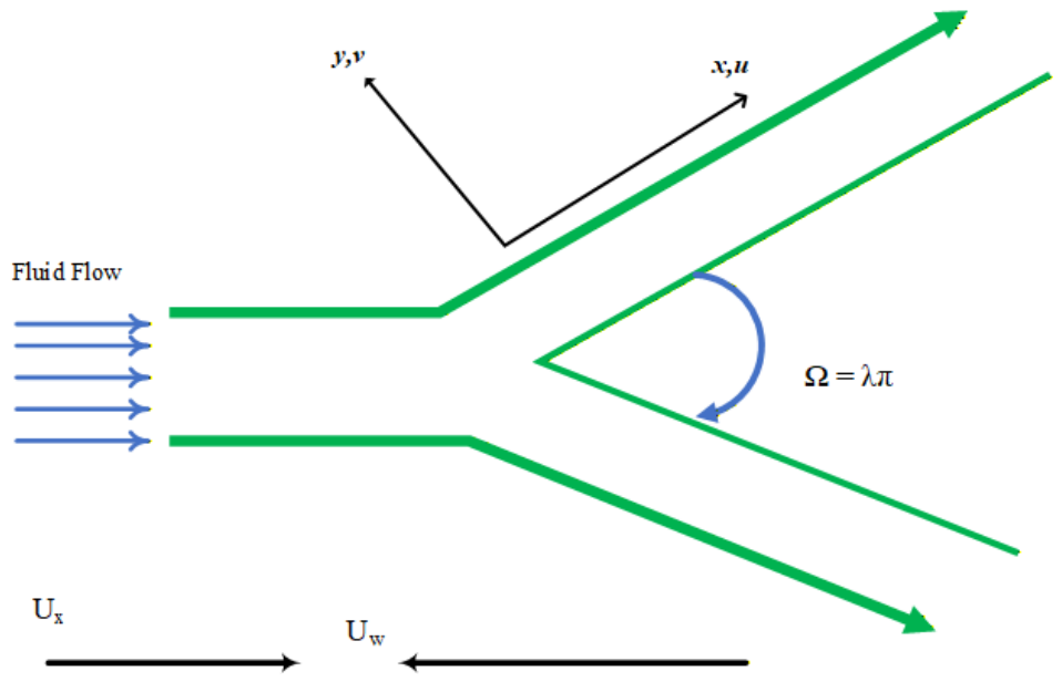
A fluid dynamic modeling is developed to examine the properties of nanomaterials. Kumar et al. [28] explored the two-dimensional, time-invariant hydrodynamic flow characteristics of a hybrid nanofluid in conjunction with a movable wedge, as depicted in Figure 1. Ω = λπ. To classify the fluid flow geometry, a Cartesian coordinate system is assumed. The wedge angle is represented by $\lambda ={\displaystyle \frac{2n}{\left(n+1\right)}}$, which serves as the parameter indicative of the wedge angle. The velocities associated with the stretching and the free stream in relation to the wedge are explicitly defined as ${\tilde{u}}_w\left(x\right)=U_w{x}^n$ and ${\tilde{U}}_e\left(x\right)=U_{\mathrm{\infty }}{x}^n$, correspondingly. The parameters ${\tilde{T}}_w$, ${\tilde{T}}_{\mathrm{\infty }}$, ${\tilde{C}}_w$, and ${\tilde{C}}_{\mathrm{\infty }}$ represent the temperature and concentration at both the boundary and throughout the free stream, respectively. The constitutive equation governing the isotropic flow behavior of a Casson fluid is expressed as follows.

$${\tau }^{1/\mathrm{N}}={{\tau }_0}^{1/\mathrm{N}}+\mu {\dot{\gamma }}^{1/\mathrm{N}},$$

(1)

$${\tau }_{ij}=\left\{\begin{array}{c}2\left({\mu }_B+{\displaystyle \frac{p_y}{\sqrt{2\pi }}}\right)e_{ij}, \pi >{\pi }_c\\ 2\left({\mu }_B+{\displaystyle \frac{p_y}{\sqrt{{\pi }_c}}}\right)e_{ij}, \pi <{\pi }_c\end{array}\right.$$

(2)

where $\pi =e_{ij}{e}_{ij}$.

The governing flow equations are:

$$D_x\tilde{u}+D_y\tilde{v}=0,$$

(3)

$$\tilde{u}{D}_x\tilde{u}+\tilde{v}{D}_y\tilde{u}={\displaystyle \frac{{\mu }_{hnf}}{{\rho }_{hnf}}}\left(\left[1+{\beta }^{-1}\right]D_{yy}\tilde{u}\right)+{\tilde{U}}_e{D}_x{\tilde{U}}_e-{\displaystyle \frac{{{\sigma }_{hnf}B}_0^2}{{\rho }_{hnf}}}\left({\tilde{U}}_e-\tilde{u}\right)+{\displaystyle \frac{{\nu }_{hnf}}{k}}\left({\tilde{U}}_e-\tilde{u}\right),$$

(4)

$$\tilde{v}{D}_y\tilde{T}+\tilde{u}{D}_x\tilde{T}+={\displaystyle \frac{{\kappa }_{hnf}}{{\left(\rho C_p\right)}_{hnf}}}{D}_{yy}\tilde{T}+{\displaystyle \frac{{\left(\rho C_p\right)}_{hnf}}{{\left(\rho C_p\right)}_f}}\left[{\displaystyle \frac{D_B}{{\delta }_c}}{D}_y\tilde{T}{D}_y\tilde{C}+{\displaystyle \frac{D_{\tilde{T}}}{{\tilde{T}}_{\infty }}}{\left(D_y\tilde{T}\right)}^2\right],$$

(5)

$$\tilde{u}{D}_x\tilde{C}+\tilde{v}{D}_y\tilde{C}=D_B{D}_{yy}\tilde{C}+{\displaystyle \frac{D_{\tilde{T}}{\delta }_c}{{\tilde{T}}_{\infty }}}{D}_{yy}\tilde{T}-{K_r}^2\left(\tilde{C}-{\tilde{C}}_{\infty }\right){\left[{\displaystyle \frac{\tilde{T}}{{\tilde{T}}_{\infty }}}\right]}^m{e}^{-\left({\displaystyle \frac{E_a}{KT}}\right)},$$

(6)

with boundary conditions

$$\tilde{u}={\tilde{u}}_w\left(x\right)=U_w{x}^n,\tilde{v}=0,\tilde{T}={\tilde{T}}_w,\tilde{C}={\tilde{C}}_w \mathrm{a}\mathrm{t} y=0,$$

(7)

$$\tilde{u}\to {\tilde{U}}_e\left(x\right)=U_{\infty }{x}^n, \tilde{T}\to {\tilde{T}}_{\infty },\tilde{C}\to {\tilde{C}}_{\infty } \mathrm{a}\mathrm{s} y\to \infty .$$

(8)

where $D_y={\displaystyle \frac{\mathsf{\partial }}{\mathsf{\partial }y}}, D_x={\displaystyle \frac{\mathsf{\partial }}{\mathsf{\partial }x}}$. $\overrightarrow{u}$ and $\overrightarrow{v}$ are the velocities along the $x$- and $y$-axes, $\beta$ is a dimensionless parameter, ${\rho }_{hnf}$ stands for fluid density, ${\mu }_{hnf}$ is the viscosity, $k$ is the permeability of the porous medium, $k*$ is the coefficient of mean absorption, $C_p$ is the specific heat capacity, $D_B$ is the Brownian diffusion coefficient, $D_{\tilde{T}}$ is the thermophoretic diffusion coefficient, ${\mu }_{hnf}$ is the viscosity, ${\delta }_c$ is a corrective factor for the molar concentration scale, $B_0$ is a material constant, $\tilde{T}$ is the fluid temperature, and ${\tilde{T}}_{\infty }$ is the free stream temperature.

The stream function $\psi$ is written as:

$$\tilde{u}=D_y\psi =, \tilde{v}=-D_x\psi .$$

(9)

Defining the transformations as the following:

$$\left.\begin{array}{c} \eta =y\sqrt{{\displaystyle \frac{{\left(n+1\right)\tilde{U}}_e}{2\nu x}}}, \psi =\sqrt{{\displaystyle \frac{{2\nu x\tilde{U}}_e}{\left(n+1\right)}}}F\left(\eta \right),\\ \theta \left(\eta \right)={\displaystyle \frac{\tilde{T}-{\tilde{T}}_{\infty }}{{\tilde{T}}_w-{\tilde{T}}_{\infty }}},\varphi \left(\eta \right)={\displaystyle \frac{\tilde{C}-{\tilde{C}}_{\infty }}{{\tilde{C}}_w-{\tilde{C}}_{\infty }}}.\end{array}\right\}$$

(10)

Implementing Equations (9) and (10) into Equations (4)–(8), the new set of equations will be as follows:

$${\left[1+{\beta }^{-1}\right]A_{1}F}^{‴}+{\lambda A_2+A_{2}FF}^{″}-{\lambda A_{2}F}^{\prime 2}+H_a{A}_3\left[{1-F}^{\prime }\right]+{\beta }_d\left[{1-F}^{\prime }\right]=0,$$

(11)

$${\displaystyle \frac{1}{P_r}}{A}_4{\theta }^{″}+A_{5}F{\theta }^{\prime }+N_b{\varphi }^{\prime }{\theta }^{\prime }+N_t{\theta }^{\prime 2}=0,$$

(12)

$${\varphi }^{″}+L_{e}F{\varphi }^{\prime }+{\displaystyle \frac{N_t}{N_b}}{\theta }^{″}-{Le\sigma }_1{\left[1+{\delta }_1\theta \right]}^{m_1}exp\left({\displaystyle \frac{-E}{1+{\delta }_1\theta }}\right)\varphi =0,$$

(13)

Boundary conditions (BCs) become

$$F^{\prime }={\gamma }_1,F=0,\varphi =1, \theta =1, \mathrm{a}\mathrm{t} \eta =0,$$

(14)

$$F^{\prime }\to 1,\theta \to 0,\varphi \to 0 \mathrm{a}\mathrm{s} \eta \to \infty .$$

(15)

where $H_a$ represents the magnetic parameter, ${\beta }_D$ the Darcy parameter, $\lambda , {\gamma }_1$ the wedge angle and wedge parameter, $P_r$ the Prandtl number, $N_t$ the thermophoresis parameter, $N_b$ the Brownian motion parameter, and $L_e$ the Lewis number. $E_1$ is the activation energy variable, $E_a$ the activation energy coefficient, ${K_r}^2$ the reaction rate, ${\delta }_1$ the temperature difference, and ${\sigma }_1$ the chemical reactive factor, which are as follows:

$$\begin{array}{l}{H}_a={\displaystyle \frac{2{\sigma }_{hnf}{B}_0^2}{{\left(n+1\right)\rho }_f{U}_{\infty }}},{\beta }_D ={\displaystyle \frac{2{\nu }_{hnf}}{\left(n+1\right)k{U}_{\infty }}}, \lambda ={\displaystyle \frac{2n}{\left(n+1\right)}}, R_e={\displaystyle \frac{{\tilde{u}}_{w}x}{{\nu }_f}},{\gamma }_1={\displaystyle \frac{U_w}{U_{\infty }}},P_r={\displaystyle \frac{{\left(\mu C_p\right)}_f}{k_f}},\\ L_e={\displaystyle \frac{{\nu }_f}{D_B}}, N_t={\displaystyle \frac{\tau D_{\tilde{T}}\left({\tilde{T}}_w-{\tilde{T}}_{\infty }\right)}{{\nu }_f{\tilde{T}}_{\infty }}}, N_b={\displaystyle \frac{{\tau D}_B}{{\delta }_c}}{\displaystyle \frac{\left({\tilde{C}}_w-{\tilde{C}}_{\infty }\right)}{{\nu }_f}}, \tau ={\displaystyle \frac{{\left(\rho C_p\right)}_{hnf}}{\rho C_p}}, E= {\displaystyle \frac{E_a}{K{\tilde{T}}_{\infty }}},\\ {\sigma }_1={\displaystyle \frac{2{K_r}^2}{\left(n+1\right){x^{n-1}U}_{\infty }}},{\delta }_1={\displaystyle \frac{{\tilde{T}}_w-{\tilde{T}}_{\infty }}{{\tilde{T}}_{\infty }}}.\end{array}$$

The nanofluid constraints are given as

$$\left.\begin{array}{c}{A}_1={\displaystyle \frac{{\mu }_{hnf}}{{\mu }_f}}={\displaystyle \frac{1}{{\left(1-{\varphi }_1-{\varphi }_2\right)}^{2.5}}},A_2={\displaystyle \frac{{\rho }_{hnf}}{{\rho }_f}}=\left(1-{\varphi }_2\right)\left[\left(1-{\varphi }_1\right)+{\displaystyle \frac{{{\varphi }_1\rho }_{1s}}{{\rho }_f}}\right]+{\displaystyle \frac{{{\varphi }_2\rho }_{2s}}{{\rho }_f}}\\ A_3={\displaystyle \frac{{\sigma }_{hnf}}{{\sigma }_f}}=\left[1+{\displaystyle \frac{3\left({\sigma }_{1s}{\varphi }_{1s}-{\varphi \sigma }_f\right){{+\varphi }_{2s}\sigma }_{2s}}{{\sigma }_{1s}\left(1-{\varphi }_{1s}\right)+{\sigma }_{2s}\left(1-{\varphi }_{2s}\right)+\left(2+\varphi \right){\sigma }_f}}\right],\\ A_4={\displaystyle \frac{k_{hnf}}{k_f}}={\displaystyle \frac{k_{2s}+2k_f-2{\varphi }_2\left(k_f-k_{2s}\right)}{k_{2s}+2k_f+{\varphi }_2\left(k_f-k_{2s}\right)}}\times k_{nf}, k_{nf}={\displaystyle \frac{k_{1s}+2k_f-2{\varphi }_1\left(k_f-k_{1s}\right)}{k_{1s}+2k_f+{\varphi }_1\left(k_f-k_{1s}\right)}},\\ A_5={\displaystyle \frac{{\left(\rho C_p\right)}_{hnf}}{{\left(\rho C_p\right)}_f}}=\left(1-{\varphi }_2\right)\left[\left(1-{\varphi }_1\right)+{\displaystyle \frac{{\varphi }_1{\left(\rho C_p\right)}_{1s}}{{\left(\rho C_p\right)}_f}}\right]+{\displaystyle \frac{{\varphi }_2{\left(\rho C_p\right)}_{2s}}{{\left(\rho C_p\right)}_f}},\phi ={\varphi }_1+{\varphi }_2 \end{array}\right\}$$

(16)

where $C_{fx}$, $N_x$, and ${Sh}_x$ are achieved as

$$\begin{array}{l}\sqrt{R_e}{C}_{fx}=\left[1+{\beta }^{-1}\right]A_1{F}^{″}\left(0\right), N_x/\sqrt{R_e}=-{\displaystyle \frac{A_4}{{\left(2/(n+1)\right)}^{0.5}}}{\theta }^{\prime }\left(0\right),\\ {Sh}_x/\sqrt{R_e}=-{\left(2/(n+1)\right)}^{-0.5}{\varphi }^{\prime }\left(0\right).\end{array}$$

(17)

$R_e$ is the Reynolds numbers.

3. The Spectral Relaxation Methodology

The spectral relaxation (SR) methodology is employed for the resolution of the nonlinear coupled differential Equations (11)–(13), with the BCs delineated in (14) and (15). We implemented the SR methodology to tackle the settled mathematical framework. The SR technique is designed to function on the system of governing differential equations that necessitates a reduction in order, as stated in Equation (11). By setting $F^{\prime }=X$, the Equations (11)–(13) are transformed accordingly.

$${\left[1+{\beta }^{-1}\right]A_{1}X}^{″}+{\lambda A_2+A_{2}FX}^{\prime }-{\lambda A_{2}X}^2+H_a{A}_3\left[1-X\right]+{\beta }_d\left[1-X\right]=0,$$

(18)

$${\displaystyle \frac{1}{P_r}}{A}_4{\theta }^{″}+A_{5}F{\theta }^{\prime }+N_b{\varphi }^{\prime }{\theta }^{\prime }+N_t{\theta }^{\prime 2}=0,$$

(19)

$${\varphi }^{″}+LeF{\varphi }^{\prime }+{\displaystyle \frac{N_t}{N_b}}{\theta }^{″}-{Le\sigma }_1{\left[1+{\delta }_1\theta \right]}^{m_1}exp\left({\displaystyle \frac{-E}{1+{\delta }_1\theta }}\right)\varphi =0,$$

(20)

Thereafter, the Gauss–Seidel relaxation technique was adopted to decompose Equations (18)–(20) in the following manner:

$${F^{\prime }}_{s+1}=X_s.$$

(21)

$$\left[1+{\beta }^{-1}\right]A_1{X″}_{s+1}+{A_{2}F}_s{X^{\prime }}_{s+1}+\lambda A_2-\lambda A_2{X_s}^2+H_a{A}_3\left[1-X_{s+1}\right]+{\beta }_d\left[1-X_{s+1}\right]=0,$$

(22)

$${\displaystyle \frac{1}{P_r}}{A}_4{{\theta }^{″}}_{s+1}+A_5{F}_{s+1}{{\theta }^{\prime }}_{s+1}+N_b{{\varphi }^{\prime }}_s{{\theta }^{\prime }}_{s+1}+N_t{{\theta }^{\prime 2}}_s=0,$$

(23)

$${{\varphi }^{″}}_{s+1}+Le{F}_{s+1}{{\varphi }^{\prime }}_{s+1}+{\displaystyle \frac{N_t}{N_b}}{\theta ″}_{s+1}-{Le\sigma }_1{\left[1+{\delta }_1\theta \right]}^{m_1}exp\left({\displaystyle \frac{-E}{1+{\delta }_1\theta }}\right){\varphi }_{s+1}=0,$$

(24)

The corresponding BCs are adjusted accordingly.

$$F_{s+1}{\left(0\right)=0, X}_{s+1}\left(0\right)={\gamma }_1,={\theta }_{s+1}\left(0\right)={\varphi }_{s+1}\left(0\right)=1 \mathrm{a}\mathrm{t} \eta =0,$$

(25)

$$X_{s+1}\left(\infty \right)\to 1,{\theta }_{s+1}\left(\infty \right)\to 0,{\varphi }_{s+1}\left(\infty \right)\to 0 \mathrm{a}\mathrm{s} \eta \to \infty .$$

(26)

In this context, the elements denoted as “$s+1$” signify the newly estimated data, whereas those marked as “$s$” indicate the previously estimated data.

The Chebyshev pseudospectral technique [29] is now employed on Equations (21)–(26), utilizing the differentiation matrix “$\mathit{D}=2/l D$” to estimate the derivatives of the acquired variables within Equations (21)–(24). As a result, we obtain

$$\mathit{D}{F}_{s+1}=X_s$$

(27)

$${\left\{diag\left[a_{0,s}\right]{A_1\mathit{D}}^2+diag\left[a_{1,s}\right]A_2\mathit{D}+diag\left[{\beta }_D+H_a+\lambda A_2\right]+diag\left[a_{2,s}\right]\mathit{I}\right\}X}_{s+1}=C_{1,s},$$

(28)

$$\begin{array}{l}\left\{{\displaystyle \frac{1}{P_r}}{A}_4{\mathit{D}}^2+A_{5}diag\left[b_{0,s}\right]\mathit{D}+N_{b}diag\left[{{\varphi }^{\prime }}_s\right]\mathit{D}+N_{t}diag\left[{{\theta }^{\prime 2}}_s\right]\right\}{\theta }_{s+1}=C_{2,s},\\ \left\{{\mathit{D}}^2+diag\left[c_{0,s}\right]\mathit{D}+diag\left[{{\theta }^{″}}_{s+1}\right]-{Le\sigma }_{1}diag\left[c_{1,s}\right]\right\}{\varphi }_{s+1}=C_{3,s},\end{array}$$

(29)

The relevant boundary conditions formulated to

$$F_{s+1}{\left({\eta }_N\right)=0, X}_{s+1}\left({\eta }_N\right)={\gamma }_1,{\theta }_{s+1}\left({\eta }_N\right)=1={\varphi }_{s+1}\left({\eta }_N\right),$$

(30)

$$X_{s+1}\left({\eta }_0\right)\to 1,{\theta }_{s+1}\left({\eta }_0\right)\to 0,{\varphi }_{s+1}\left({\eta }_0\right)\to 0.$$

(31)

The pertinent earliest hypotheses are delineated are:

$$F_0\left(\eta \right)=\eta +\left({\gamma }_1-1\right)\left(1-e^{-\eta }\right), { X}_0\left(\eta \right)=1+\left({\gamma }_1-1\right)e^{-\eta }, { \theta }_0\left(\eta \right)={\varphi }_0\left(\eta \right)= e^{-\eta }.$$

(32)

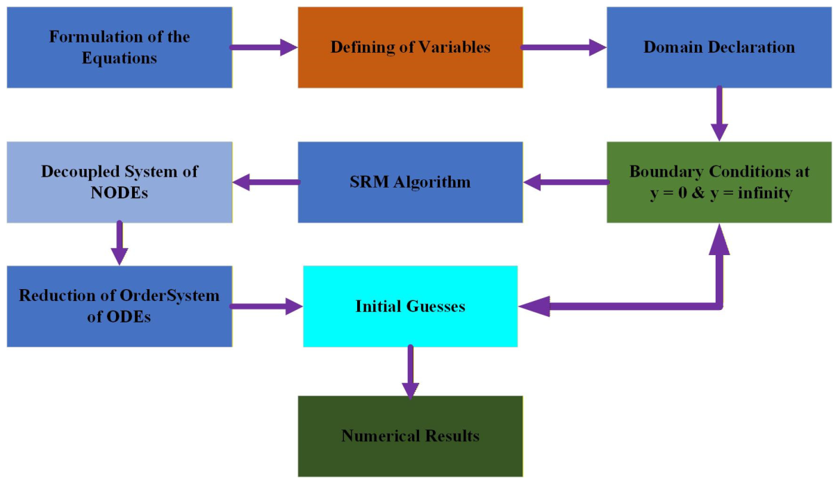
These initial hypotheses (guesses) fulfill the boundary conditions (30) and (31) and subsequently facilitate the determination of the approximated values for $F_s, X_s, {\theta }_s, {\varphi }_s$ of each variable through the application of the SR technique. The algorithm presently used has been created and run through the computational program MATLAB. Refer to Figure 2 for a comprehensive depiction of the simulation process.

Convergence, Error, and Stableness of the Iteration Scheme

The convergence and stability of the present iterative methodology can be assessed by considering the norms of the variations in function values across two successive iterations. Consequently, for each iteration, the maximum error ($E_{rr}$) associated with the ($s+1$)th iteration is defined as:

$$E_{rr}=Max(F_{1,s+1}-F_{1,s\infty },F_{2,s+1}-F_{2,s\infty }, \dots , F_{m,s+1}-F_{m,s\infty }).$$

(33)

In instances where the numerical outcomes from the iterations exhibit convergence, it is anticipated that the error $E_{rr}$ will diminish with an increase in subsequent iterations.

The unknowns were approximated over a series of collocation points, denoted as $\mathrm{N}$, until the convergence criterion articulated below was fulfilled at iteration $s$

$$E_{rr}\le {\epsilon }_1.$$

(34)

where ${\epsilon }_1$ represents the threshold for convergence tolerance. The convergence tolerance criterion for the present study is established at ${\epsilon }_1={10}^{-6}$. The influence of the number of collocation points N is examined to identify the minimal values of $N$ that yield consistent solutions within the established ${\epsilon }_1$ error tolerance. This is achieved through the iterative resolution of the governing equations utilizing the proposed iterative scheme with varying values of $N$ until coherent solutions are attained.

To demonstrate the numerical accuracy and convergence of the proposed SR scheme, a collocation-point independence study was carried out by progressively increasing the number of Chebyshev collocation points ($N$). The governing equations were solved repeatedly for distinct values of ($N$), and the engineering quantities of practical interest, like the skin-friction coefficient ($F^{″}\left(0\right)$), the local Nusselt number ($-{\theta }^{\prime }\left(0\right)$), and the local Sherwood number ($-{\varphi }^{\prime }\left(0\right)$), were recorded. It was noted that the numerical solutions converge rapidly as ($N$) increases, with the relative difference between successive refinements falling below the prescribed tolerance of (${\epsilon }_1={10}^{-6}$). Beyond ($N=80$), no noticeable variation was observed in the computed boundary-layer profiles, confirming mesh independence and numerical stability. Consequently, ($N=80$) was adopted in all subsequent simulations to ensure an appropriate balance between computational efficiency and numerical accuracy.

4. Results and Discussion

The subsequent segment elucidates the graphical depictions and quantitative findings derived from the SR methodology in relation to an array of physical parameters. This segment offers a comprehensive examination of the fluctuations of several emergent parameters linked to the functions of velocity, temperature, and concentration.

4.1. Tabular Results

Table 1. Comparative numerical stipulated antecedent results of the skin drag coefficient $C_{fx}$ based on stipulating ${\beta }_d=0$.

${\mathit{H}}_{\mathit{a}}$	$\mathit{\beta }$	$\mathit{\lambda }$	${\mathit{\gamma }}_1$	Current Results for ${\mathit{C}}_{\mathit{f}\mathit{x}}$	Swami et al. [30]
1	0.2	1	0.1	−0.132937	−0.132937
2	0.2	1	0.1	−0.157845	−0.157844
3	0.2	1	0.1	−0.179024	−0.179023
1	−0.2	1	0.1	−0.186815	−0.186813
1	0	1	0.1	−0.161034	−0.161033
1	0.2	1	0.1	−0.132938	−0.132937
1	0.2	1	0.1	−0.148499	−0.148498
1	0.2	2	0.1	−0.190527	−0.190525
1	0.2	3	0.1	−0.238906	−0.238906
1	0.2	1	0.1	−0.132937	−0.132937
1	0.2	1	0.2	−0.133486	−0.133485
1	0.2	1	0.3	−0.135242	−0.135241

and

Table 2. Comparative numerical stipulated antecedent results of the Nusselt number $N_x$ based on stipulating ${\beta }_d=0, N_t=0.1, N_b=1$.

${\mathit{H}}_{\mathit{a}}$	$\mathit{\beta }$	$\mathit{\lambda }$	${\mathit{\gamma }}_1$	Current Results for ${\mathit{N}}_{\mathit{x}}$	Swami et al. [30]
1	0.2	1	0.1	0.937814	0.937814
2	0.2	1	0.1	0.956957	0.956958
3	0.2	1	0.1	0.972591	0.972590
1	−0.2	1	0.1	0.875998	0.875997
1	0	1	0.1	0.907091	0.907090
1	0.2	1	0.1	0.937814	0.937814
1	0.2	1	0.1	0.950791	0.950790
1	0.2	2	0.1	0.983881	0.983883
1	0.2	3	0.1	1.019179	1.019179
1	0.2	1	0.1	0.470883	0.470882
1	0.2	1	0.2	0.469705	0.469706
1	0.2	1	0.3	0.467846	0.467847

provide a comparative analysis of the results and an evaluation of the trends observed in the skin friction and Nusselt number profiles. Table 1, Table 2 and

Table 3. Comparative numerical stipulated antecedent results of the Sherwood number ${Sh}_x$ based on stipulating ${\beta }_d=0, N_t=0.1, N_b=1$, ${\delta }_1={\sigma }_1=E=0$.

${\mathit{H}}_{\mathit{a}}$	$\mathit{\beta }$	$\mathit{\lambda }$	${\mathit{\gamma }}_1$	Current Results for ${\mathit{S}\mathit{h}}_{\mathit{x}}$	Swami et al. [30]
1	0.2	1	0.1	0.164492	0.164492
2	0.2	1	0.1	0.160888	0.160890
3	0.2	1	0.1	0.156419	0.156417
1	−0.2	1	0.1	0.127532	0.127531
1	0	1	0.1	0.147013	0.147014
1	0.2	1	0.1	0.164490	0.164492
1	0.2	1	0.1	0.950791	0.162666
1	0.2	2	0.1	0.153406	0.153405
1	0.2	3	0.1	0.137451	0.137452
1	0.2	1	0.1	1.198821	1.198822
1	0.2	1	0.2	1.333973	1.333972
1	0.2	1	0.3	1.045376	1.045377

demonstrate changes in $C_{fx}$, ${Sh}_x$, and $N_x$ across the different parameters $H_a,\beta , \lambda , {\gamma }_1$. The $C_{fx}$ is promoted through increasing the $H_a,\beta , \lambda , {\gamma }_1$, and both the $N_x$, ${Sh}_x$ are anticipated to be positive with the increase in said parameters.

4.2. Velocity Profile

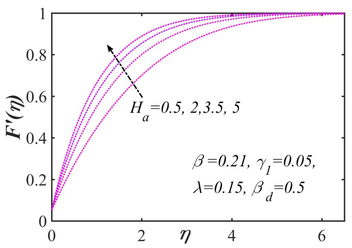
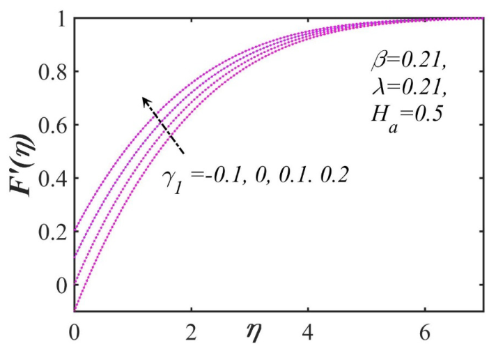
Figure 3 reveals the impact of $H_a$ on $F^{\prime }$. The Hartmann layer, also known as the diffusive layer, appears when a magnetic field is present, which causes the Lorentz force. The layer diminishes the retarding force on the velocity field of the hybrid nanofluid by lowering the momentum boundary layer thickness whenever enhancing the magnetic parameter $H_a$. The presence of the layer mitigates the opposing force acting on the velocity field of the hybrid nanofluid by diminishing the momentum boundary layer thickness through an elevation in the magnetic parameter “$H_a$”. Thus, as a result of the diminished retarding force, the flow velocity of the hybrid nanofluid traversing a wedge-shaped surface is augmented as the value of $H_a$ escalates. These findings elucidate that the velocity is markedly affected by an increase in the $H_a$. Figure 4 portrays the impact of ${\gamma }_1$ over $F^{\prime }$ distribution. The $F^{\prime }$ value exhibits an increment as the wedge parameter ascends, thereby inducing the fluid to move in opposition to the shear stress present alongside the subsurface.

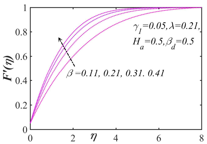
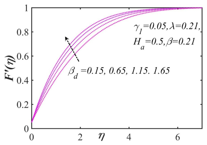
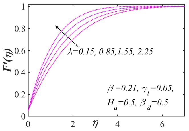
Figure 5 illustrates the implications of the porosity parameter ${\beta }_d$ on the flow dynamics. Enlarging ${\beta }_d$ values causes an elevation in the velocity distribution and also reduces the thickness of the boundary layer. Figure 6 delineates the repercussions of $\beta$ on the dispersions of $F_{\prime }$. The $F_{\prime }$ profile of hybrid fluids is lifted as the value of $\beta$ increases. Notably, the velocity profile of the hybrid nanofluid evidences a marked enhancement with the incorporation of hybrid nanofluid. This is because it exhibits an inverse correlation with fluid viscosity: an increase in the values of $\beta$ will lead to a decrease in fluid viscosity, thus increasing the stress rate in the boundary layer. The orientation of a moving wedge exerts a significant influence on the modulation amplitude of velocity, temperature, and concentration profiles within the domains of fluid dynamics and heat/mass transfer phenomena. Figure 7 is presented to analyze the effect of the wedge angle $\lambda$ on the $F^{\prime }$ profile. An elevation in the wedge angle parameter results in an elevation of the $F^{\prime }$ profile. This phenomenon can be attributed to the observation that a steeper wedge (i.e., a higher wedge angle) correlates with increased velocities around the leading edge of the wedge, which arise from augmented pressure gradients. The velocity profile along the surface may manifest a more pronounced alteration (gradient) as the wedge angle escalates.

4.3. Temperature Profile

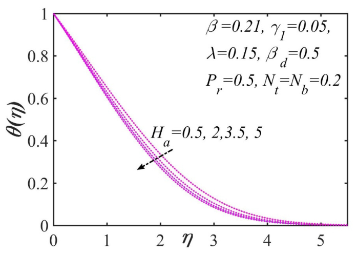
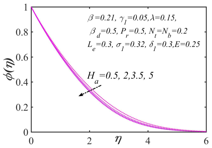
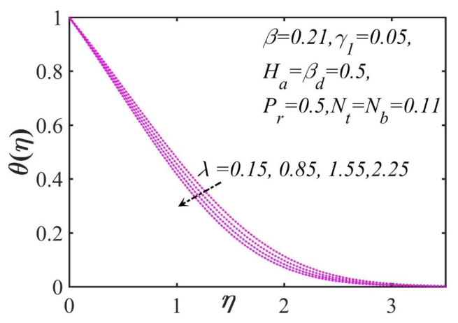
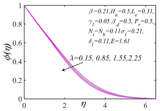
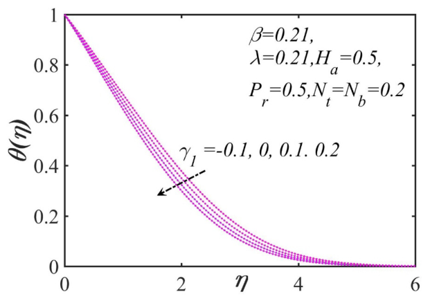
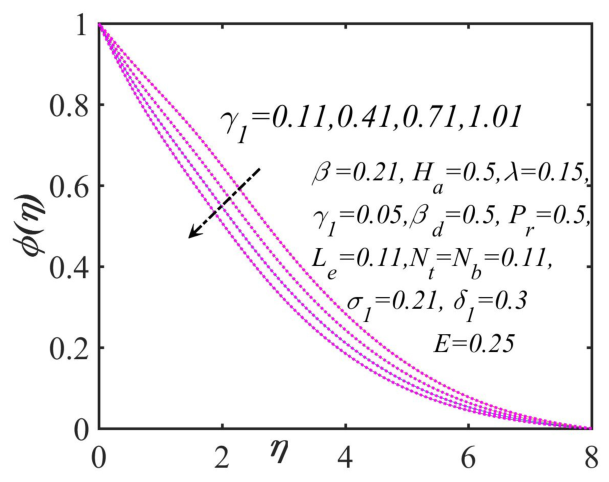
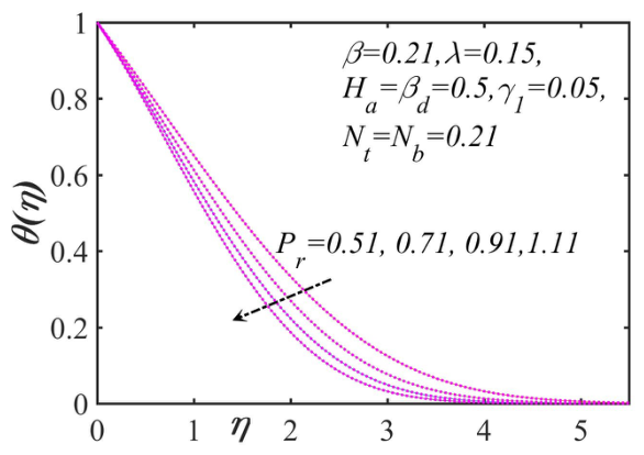
Figure 8 and Figure 9 explain how the $\theta \left(\eta \right), \varphi \left(\eta \right)$ in the boundary layer change under the influence of the magnetic parameter $H_a$, in the condition of a sheet being stretched. The profiles of $\theta \left(\eta \right), \varphi \left(\eta \right)$ exhibit a decrement in response to an augmentation of the magnetic field contrast to $F^{\prime }\left(\eta \right)$. An increase in $H_a$ enhances the temperature and concentration distributions within the boundary layer. This occurs because the Lorentz force opposes the fluid motion, reducing the flow velocity and increasing the residence time of the fluid near the wedge surface. Consequently, heat accumulates within the fluid, resulting in higher temperatures and thicker thermal and concentration boundary layers, while the effective density of the hybrid nanofluid near the convective wedge surface decreases due to thermal expansion. Figure 10, Figure 11, Figure 12 and Figure 13 are presented to analyze the effect of the wedge angle $\lambda$ and ${\gamma }_1$ on $\theta \left(\eta \right)$ and $\varphi \left(\eta \right)$. When the $\lambda$ values augmented, simultaneously decreasing the profiles of both $\theta \left(\eta \right)$ and $\varphi \left(\eta \right)$ are recorded. Additionally, an increase in the wedge angle modifies the surface region disclosed to the fluid flow, thereby impacting heat transfer rates, temperature, and concentration profiles. A faster fluid movement near the surface which is caused by $\lambda$ enhances convectional heat transfer, thus dominating conductive processes and the effects of mass transfer. The parametric quantities $\theta \left(\eta \right)$ and $\varphi \left(\eta \right)$ are noticed to diminish with the increase in the wedge parameter ${\gamma }_1$. The temperature inside the system is lowered at the wedge subsurface, and meanwhile, an escalation in the wedge parameter results in the thermal boundary layer thickness when the temperature of the fluid closer to the surface is ready for heat dissipation. From Figure 14, it is recorded that an enhancement in $P_r$ produces a decrement in $\theta \left(\eta \right)$ and also in thermal boundary layer thickness due to the phenomenon where raising the values brings decrement in thermal conductivity. Therefore, a fluid described by an elevated $P_r$ demonstrates a lesser thermal boundary layer thickness.

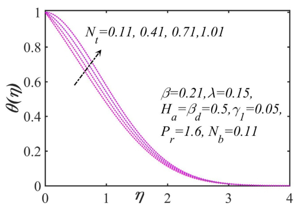
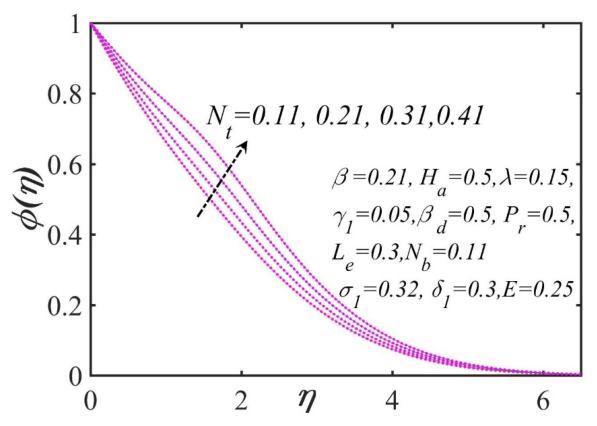
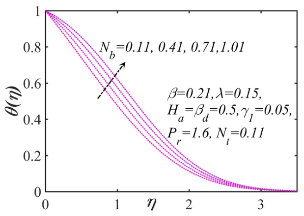
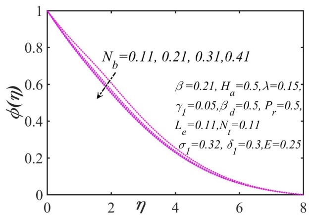
Figure 15 and Figure 16 elucidate the impact of the thermophoretic parameter on profiles $\theta \left(\eta \right)$ and $\varphi \left(\eta \right)$. It is discerned that an increase in $N_t$ serves to enhance both $\theta \left(\eta \right)$ and $\varphi \left(\eta \right)$. The thermophoretic parametric quantity fosters an elevation in temperature and concentration profiles, as was previously observed. Consequently, the warmer fluid is propelled away from the surface, leading to an increase in temperature within the boundary layer as $N_t$ escalates. This increase in profiles is credited to the thermophoretic force available due to the temperature gradient that drives high-velocity flow along the surface. Figure 17 and Figure 18 delineate the alterations in $\theta \left(\eta \right)$ and $\varphi \left(\eta \right)$ profiles induced by Brownian motion $N_b$. It has been established that the temperature of the fluid elevates in response to the $N_b$ parameter. Due to their elevated Brownian velocity and relatively higher particle diffusivity, smaller particles (less than 5 nm) exhibit enhanced thermal conductivities. In contrast, particles with sizes exceeding 10 nm demonstrate considerable repulsion coupled with minimal random diffusion. Meanwhile, its concentration decreases with the larger number of $N_b$. In physical terms, $N_b$ facilitates the dispersion and erratic movement of particles within the fluid, thereby enhancing thermal distribution; consequently, the fluid temperature increases, leading to a gradual decline in $\varphi \left(\eta \right)$.

4.4. Concentration Profile

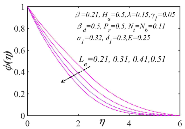
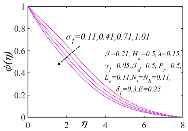
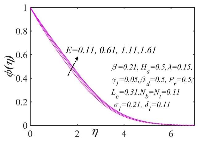
Figure 19 illustrates the impact of the Lewis number on the concentration profile. The findings indicate that an increase in the Lewis number results in a more homogeneous concentration magnitude, implying a reduction in the diffusion rate. The implications of the chemical reaction constant ${\sigma }_1$ and the activation energy parameter ($E$) are depicted in Figure 20 and Figure 21, which illustrate that $\varphi \left(\eta \right)$ diminishes with the escalation of ${\sigma }_1$, whereas it increases with the rise in the numerical value of $E$. Moreover, the appearance of other phenomena like Brownian motion and thermophoresis is essentially critical in the distribution of nanoparticles in a fluidic medium and thus affects thermal conductivity and viscosity. The relationship between concentration fluctuations and physical properties is of utmost significance for the engineering of systems in which the effective management of nanoscale particles is essential for the optimization of processes, such as pharmaceutical delivery or enhanced thermal transfer. The given graphs are approaching a graceful profile in the free stream area smoothly, which proves that the chosen SR hypotheses satisfy the boundary conditions at infinity. This assures the flexibility of the mathematical model and its relevance to the investigated flow and concentration phenomena. The findings of this study can also support engineers in enhancing cooling performance in heat exchangers, electronic cooling devices, energy storage systems, polymer processing, and MHD-assisted manufacturing processes. In addition, the numerical results provide practical design guidance for increasing heat transfer efficiency, lowering energy consumption, and improving the operational reliability of thermal systems that use hybrid nanofluids under complex flow conditions.

5. Concluding Remarks

This article examines the flow dynamics and heat transfer properties of a hybrid nanofluid consisting of Al₂O₃, CuO, and ethylene glycol over a porous wedge-shaped subsurface undergoing horizontal elongation, which are affected by activation energy, thermophoresis, Brownian motion, and magnetic fields. The SR scheme is employed to solve the governing nonlinear equations of the flow operating similarity transformations and their associated boundary conditions in MATLAB. The findings are presented in the form of graphical illustrations, with an analysis of the comparison with the previous research findings. The main findings of the present investigation are:

• The velocity is markedly affected by an increase in the $H_a$. In contrast, the profiles of $\theta \left(\eta \right), \varphi \left(\eta \right)$ exhibit a decrement in response to an augmentation of the magnetic field. The magnetic force modifies the fluid motion while suppressing thermal and species transport, resulting in lower temperature and concentration profiles.
• The $F^{\prime }$ value exhibits an increment as the wedge parameter ascends, thereby inducing the fluid to move in opposition to the shear stress present at the surface.
• When the parametric quantities $\beta ,$ ${\beta }_D$ are elevated, the velocity distribution graph rises, accompanied by a reduction in velocity boundary layer thickness.
• An elevation in the wedge angle parameter $\lambda$ results in an elevation of the $F^{\prime }$ profile, where a simultaneous decreasing effect of both $\theta \left(\eta \right)$ and $\varphi \left(\eta \right)$ are recorded.
• An increase in the Prandtl number $P_r$ results in a reduction in the fluid temperature $\theta \left(\eta \right)$, demonstrating a lesser thickness of the thermal boundary layer.
• The thermophoretic parameter $N_t$ engenders an elevation on either side of temperature and concentration profiles.
• The fluid temperature $\theta \left(\eta \right)$ increases with a larger numeric of the Brownian motion parameter $N_b$, while its concentration decreases with a larger number of $N_b$.
• The $\varphi \left(\eta \right)$ diminishes with the escalation of ${\sigma }_1$, whereas it increases with the rise in the numerical value of $E$.
• The SRM model exhibits remarkable computational accuracy and robust numerical stability when applied to nonlinear boundary value problems frequently encountered in multiphysics reactive magneto-rheological nanofluid-assisted materials processing on complex surfaces.

References

1. Sakiadis, B.C. Boundary layer behavior on continuous solid surfaces: Boundary-layer equations for two-dimensional and axisymmetric flow. AIChE J. 1961, 7, 26–28. [Google Scholar] [CrossRef]
2. JEastman, A.; Phillpot, S.R.; Choi, S.U.S.; Keblinski, P. Thermal transport in nanofluids. Annu. Rev. Mater. Res. 2004, 34, 219–246. [Google Scholar] [CrossRef]
3. Prasher, R.; Song, D.; Wang, J.; Phelan, P. Measurements of nanofluid viscosity and its implications for thermal applications. Appl. Phys. Lett. 2006, 89, 133108. [Google Scholar] [CrossRef]
4. Das, S.K.; Choi, S.U.S.; Yu, W.; Pradeep, T. Nanofluids: Science and Technology; Wiley: Hoboken, NJ, USA, 2007. [Google Scholar]
5. Buongiorno, J.; Hu, L.-W. Nanofluid coolants for advanced nuclear power plants. In Proceedings of the ICAPP’05, Seoul, Republic of Korea, 15–19 May 2005. [Google Scholar]
6. Buongiorno, J. Convective transport in nanofluids. J. Heat Transf. 2006, 128, 240–250. [Google Scholar]
7. Abbas, N.; Shatanawi, W. Theoretical survey of time-dependent micropolar nanofluid flow over a linear curved stretching surface. Symmetry 2022, 14, 1629. [Google Scholar] [CrossRef]
8. Nadeem, S.; Abbas, N.; Malik, M. Inspection of hybrid based nanofluid flow over a curved surface. Comput. Methods Programs Biomed. 2020, 189, 105193. [Google Scholar] [CrossRef] [PubMed]
9. Shahid, A.; Huang, H.; Bhatti, M.; Marin, M. Numerical computation of magnetized bioconvection nanofluid flow with temperature-dependent viscosity and Arrhenius kinetic. Math. Comput. Simul. 2022, 200, 377–392. [Google Scholar] [CrossRef]
10. Shamshuddin, M.D.; Panda, S.; Umavathi, J.C.; Mishra, S.R.; Alruwaili, A.S.; Eid, M.R. Diversified characteristics of the dissipative heat on the radiative micropolar hybrid nanofluid over a wedged surface: Gauss-Lobatto IIIA numerical approach. Alex. Eng. J. 2024, 106, 448–459. [Google Scholar] [CrossRef]
11. Elsaid, E.M.; Eid, M.R.; Elnaggar, G.R.; El-Aziz, M.A. Hall-induced Cattaneo-Christov effects on Carreau nanofluid flow across a stretchable vertical wedge with an inclined magnetic field. Chin. J. Phys. 2026, 101, 432–450. [Google Scholar] [CrossRef]
12. Tiwari, R.K.; Das, M.K. Heat transfer augmentation in a two-sided lid-driven differentially heated square cavity utilizing nanofluids. Int. J. Heat Mass Transf. 2007, 50, 2002–2018. [Google Scholar] [CrossRef]
13. Ibrahim, W. MHD boundary layer flow and heat transfer of micropolar fluid past a stretching sheet with second-order slip. J. Braz. Soc. Mech. Sci. Eng. 2017, 39, 791–799. [Google Scholar] [CrossRef]
14. Ullah, Z.; Abbas, A.; El-Zahar, E.R.; Seddek, L.F.; Akgul, A.; Hassan, A.M. Significance of thermal density and viscous dissipation on heat and mass transfer of chemically reactive nanofluid flow along a stretching sheet under a magnetic field. Results Eng. 2023, 20, 101413. [Google Scholar] [CrossRef]
15. Hashim, H.; Hafeez, M.; Chu, Y.M. Numerical simulation for heat and mass transport analysis for magnetic nanofluid flow through stretchable convergent/divergent channels. Int. J. Mod. Phys. B 2021, 35, 2150198. [Google Scholar] [CrossRef]
16. Sohail, A.; Hang, X. Mixed convection in gravity-driven thin nanoliquid film flow with homogeneous–heterogeneous reactions. Phys. Fluids 2020, 32, 023604. [Google Scholar] [CrossRef]
17. Daniel, Y.S.; Aziz, Z.A.; Ismail, Z.; Salah, F. Entropy analysis in electrical magnetohydrodynamic (MHD) flow of nanofluid with effects of thermal radiation, viscous dissipation, and chemical reaction. Theor. Appl. Mech. Lett. 2017, 7, 235–242. [Google Scholar] [CrossRef]
18. Mulinti, V.R.; Pallavarapu, L. Influence of thermal radiation and viscous dissipation on MHD flow of UCM fluid over a porous stretching sheet with higher-order chemical reaction. Spec. Top. Rev. Porous Media Int. J. 2021, 12, 33–49. [Google Scholar] [CrossRef]
19. Wakif, A.; Abderrahmane, A.; Guedri, K.; Bouallegue, B.; Kaewthongrach, R.; Kaewmesri, P.; Jirawattanapanit, A. Importance of exponentially falling variability in heat generation on chemically reactive von Kármán nanofluid flows subjected to a radial magnetic field. Front. Phys. 2022, 10, 988275. [Google Scholar] [CrossRef]
20. Vinodkumar, M.; Reddy, P. Higher-order chemical reaction and radiation effects on magnetohydrodynamic flow of a Maxwell nanofluid with Cattaneo–Christov heat flux model over a stretching sheet in a porous medium. J. Fluids Eng. 2022, 144, 041204. [Google Scholar] [CrossRef]
21. Yahaya, S.D.; Aliyu, U.; Umaru, H. Stagnation point flow with thermal and magnetic field over a stretching sheet. Sci. World J. 2022, 17, 191–199. [Google Scholar]
22. Shahid, A.; Miao, Z.; Mahmood, A.; Shafique, M.; Khan, A. MHD nanofluid boundary layer flow through a stretching surface along with permeable media and activation energy. Cogent Eng. 2025, 12, 2582949. [Google Scholar] [CrossRef]
23. Sohail, M.; Alrabaiah, H.; Nazir, U. Radiative flow of MHD non-Newtonian fluid utilizing an updated heat flux model under Joule heating. Heat Transf. 2021, 50, 3407–3425. [Google Scholar] [CrossRef]
24. Waseem, F.; Sohail, M.; Ilyas, N.; Awwad, E.M.; Sharaf, M.; Khan, M.J.; Tulu, A. Entropy analysis of MHD hybrid nanoparticles with OHAM considering viscous dissipation and thermal radiation. Sci. Rep. 2024, 14, 1096. [Google Scholar] [CrossRef] [PubMed]
25. Khan, M.A.; Sun, J.; Li, B.; Przybysz, A.; Kosel, J. Magnetic sensors: A review and recent technologies. Eng. Res. Express 2021, 3, 022005. [Google Scholar] [CrossRef]
26. Ijaz, N.; Zeeshan, A.; Batool, S.; Bhatti, M.M.; Mekheimer, K.S. Three-dimensional multiphase peristaltic flow through a porous medium with compliant boundary walls. Contemp. Math. 2024, 5, 4874–4889. [Google Scholar] [CrossRef]
27. Elsaid, E.M.; El-Aziz, M.A.; Alruwaili, A.S.; Eid, M.R. Physical aspects of radiative Carreau nanofluid flow with motile microorganisms movement under yield stress via oblique penetrable wedge. Nanotechnol. Rev. 2025, 14, 20250146. [Google Scholar] [CrossRef]
28. Kumar, A.; Ray, A.K.; Saha, S.; Tanwar, D.V.; Kumar, B.; Sheremet, M.A. Flow of hybrid nanomaterial over a wedge: Shape factor of nanoparticles impact. Eur. Phys. J. Plus 2023, 138, 901. [Google Scholar] [CrossRef]
29. Trefethen, L.N. Spectral Methods in MATLAB; Society for Industrial and Applied Mathematics (SIAM): Philadelphia, PA, USA, 2000. [Google Scholar]
30. Swami, S.; Biradar, S.; Tawade, J.V.; Govindan, V.; Byeon, H.; Pimpunchat, B. Brownian motion effects and thermophoresis on heat transmission mechanism of hybrid nanoliquid flow over a stretched wedge surface. Partial. Differ. Equ. Appl. Math. 2025, 14, 101157. [Google Scholar] [CrossRef]
Figure 1. Flow configuration.
Mca 31 00143 g001
Figure 2. Flow chart for generating numerical results.
Mca 31 00143 g002
Figure 3. Effectiveness of H a on velocity magnitudes.
Mca 31 00143 g003
Figure 4. Impact of γ 1 on velocity distribution.
Mca 31 00143 g004
Figure 5. Influences of β on velocity profile.
Mca 31 00143 g005
Figure 6. Consequences of β d velocity pattern.
Mca 31 00143 g006
Figure 7. Effects of λ velocity pattern.
Mca 31 00143 g007
Figure 8. Aftereffects of H a on temperature magnitudes.
Mca 31 00143 g008
Figure 9. Effects of H a on concentration pattern.
Mca 31 00143 g009
Figure 10. Influences of λ on temperature pattern.
Mca 31 00143 g010
Figure 11. Impact of λ on concentration pattern.
Mca 31 00143 g011
Figure 12. Effectiveness of γ 1 on temperature pattern.
Mca 31 00143 g012
Figure 13. Influences of γ 1 on concentration magnitudes.
Mca 31 00143 g013
Figure 14. Impact of P r on temperature pattern.
Mca 31 00143 g014
Figure 15. Effects of N t on temperature profile.
Mca 31 00143 g015
Figure 16. Effects of N t on concentration pattern.
Mca 31 00143 g016
Figure 17. Impact of N b on temperature pattern.
Mca 31 00143 g017
Figure 18. Effectiveness of N b on concentration pattern.
Mca 31 00143 g018
Figure 19. Consequences of L e on concentration pattern.
Mca 31 00143 g019
Figure 20. Consequences of σ 1 on concentration pattern.
Mca 31 00143 g020
Figure 21. Consequences of E on concentration pattern.
Mca 31 00143 g021