Nonlinear Dynamic Stability Analysis of a Human-Inspired Electromechanical Arm System Under Heavy External Loads

Abstract

This study develops a nonlinear dynamic model of a human-inspired electromechanical arm system subjected to high loads. The proposed simplified representation preserves essential nonlinear dynamics using a reduced number of generalized coordinates. The model is represented by an electromechanical analog comprising a DC motor, a transmission system, and a multi-degree-of-freedom mechanical structure. The formulation is based on Lagrangian mechanics and accounts for inertia, damping, stiffness, and nonlinear kinematic coupling induced by joint misalignment. The numerical results were assessed using a consistency-based verification approach with several independent nonlinear analysis tools. The Lyapunov exponent was used in conjunction with bifurcation diagrams, Poincaré maps, and FFT spectra to identify the transition from stable operation to chaotic behavior as the external load increased. The results reveal a progressive transition from periodic motion to quasi-periodic oscillations and chaotic regimes, with fully developed chaotic behavior emerging for loads exceeding approximately 35 kg. Analysis of the Lyapunov exponent supports this interpretation, indicating stable, quasi-critical, or chaotic regimes depending on the sign of λ_max. The concordance among these independent indicators provides numerical verification of the observed stability transitions. The control gain significantly influences energy dissipation and system stability. The proposed model provides a reduced-order framework for studying nonlinear stability phenomena in human-inspired electromechanical systems. Potential applications involve rehabilitation devices and safety studies of human–robot interactions.

1. Introduction

Human–robot interaction systems have attracted considerable interest in recent years due to their increasing importance in rehabilitation engineering, assistive robotics, and collaborative industrial applications. The human-inspired electromechanical arm system, characterized by rigid articulated segments and soft biological tissues, exhibits complex nonlinear dynamic behavior when subjected to external loads or vibrating environments. In robotics, electromechanical analogs are frequently used to reproduce the functional behavior of biological systems. These systems integrate mechanical structures, actuators, and control strategies to ensure their stability and performance under uncertain conditions. Impedance and admittance control approaches have been widely used to regulate interaction forces in human–robot systems, ensuring compliance and safety [1,2]. More recent developments have introduced adaptive and nonlinear control schemes capable of handling time-varying interaction dynamics [3]. Despite these advances, the effect of a large external load on the nonlinear stability of coupled electromechanical systems remains poorly understood, particularly in systems exhibiting geometric nonlinearities and coupled electromechanical behavior. Nonlinear analysis tools, such as bifurcation diagrams and Poincaré maps, offer a robust framework for identifying transitions between stable, quasi-periodic, and chaotic regimes [4,5,6]. From a theoretical point of view, nonlinear mechanical systems subjected to an increasing energy input often exhibit a sequence of transitions governed by bifurcation theory, including period-doubling pathways to chaos [7]. In robotic arm systems, these transitions are strongly influenced by joint compliance, actuator dynamics, and load-dependent inertia [8]. A major challenge in human–robot interaction lies in designing control strategies that guarantee both performance and safety under various operational conditions. In this regard, compliance with safety standards and interaction constraints is considered an essential condition for the success of physical human–robot collaboration [9]. However, beyond the control design, the intrinsic dynamic behavior of the coupled human–robot system must be carefully analyzed, especially when subjected to external loads that may induce non-linear responses.

Recent studies have shown that human interaction can significantly influence the stability of robotic systems, especially when interaction forces are variable and uncertain [10]. These effects are even more pronounced in systems exhibiting geometric nonlinearities, joint compliance, and transmission dynamics. Under these conditions, the system can exhibit complex dynamic behaviors, including multi-frequency oscillations, bifurcations, and even chaotic movement. Nonlinear dynamic analysis offers a robust framework for studying these phenomena. Bifurcation analysis makes it possible to identify the critical thresholds of parameters associated with qualitative changes in system behavior, such as transitions from a periodic regime to a quasi-periodic or chaotic regime. Complementary tools, such as Poincaré diagrams, allow for a geometric characterization of the system’s trajectories and facilitate the detection of instabilities. The combined use of these techniques offers a comprehensive approach to understanding the evolution of system dynamics under different conditions. In this context, recent work has demonstrated the relevance of combining bifurcation analysis with phase-space methods to improve the prediction and interpretation of instability mechanisms in coupled systems [11].

Recent advances in biomechanics and rehabilitation robotics have demonstrated that upper-limb systems must be analyzed as coupled human–machine dynamic systems exhibiting highly nonlinear behaviors. The work in [12] highlighted the importance of dynamic models capable of reproducing the complex interactions between the user and robotic upper limb rehabilitation devices. Similarly, Guatibonza et al. [13] showed that the design of effective rehabilitation robots requires a realistic representation of joint inertias, passive segment properties, and energy dissipation mechanisms. Recent studies in [14,15] also indicate that dynamic stability, mechanical compliance, and control of the human–robot interaction are essential factors for ensuring the safety and effectiveness of robotic systems designed for motor assistance. Furthermore, Zhou et al. [16] demonstrated that the geometric and passive properties of the upper limb directly influence the stability of human–robot physical interactions. In this context, the electromechanical model proposed in this study aims to provide a simplified but physically consistent framework for analyzing the influence of external loads on the overall stability of a system inspired by the human-inspired electromechanical arm system, while highlighting bifurcation mechanisms and transitions to chaotic behavior under high stress.

The influence of heavy external loading on the nonlinear dynamic behavior of electromechanical analogs of the human-inspired electromechanical arm system remains insufficiently explored. In particular, there is a lack of simplified yet physically consistent models capable of capturing global stability transitions without resorting to highly detailed musculoskeletal formulations. The model incorporates a DC motor actuation system, transmission effects, and a multi-degree-of-freedom mechanical structure with nonlinear joint coupling. The formulation, developed using Lagrangian mechanics, is specifically designed to capture the overall dynamic response of the system under different external loads.

The objective of this work is not to reproduce realistic human lifting capacities, but rather to study nonlinear stability transitions in a human-inspired electromechanical system subjected to progressively increasing external loads. In doing so, the novelty of this study lies in the integration of a simplified electromechanical arm model, combining the dynamics of a DC motor with a nonlinear joint coupling. This framework allows for rigorous analysis of bifurcations as a function of load and stability assessments under high external loads while contributing to a better understanding of nonlinear dynamics in coupled electromechanical systems. The article is structured as follows: Section 2 presents the dynamic modeling of the electric motor controlling the arms, establishes the complete formulation of the robot-arm system, integrating the flexible joints into the model. Section 3 presents the numerical results obtained from simulations carried out with a set of specific parameters to validate the behavior of the proposed model. Finally, Section 4 concludes the study by summarizing the main contributions and opening perspectives for future research.

2. Comprehensive Description of the Electromechanical Hand–Arm System with an Integrated Mechanical Control System

2.1. Positioning of This Work

The present work differs from previous studies in three main aspects: it establishes a unified nonlinear framework that integrates electromechanical with a simplified dynamic representation of the upper limb, explicitly analyzes load-induced bifurcation behaviors within this coupled system, and prioritizes a global perspective of system stability rather than focusing solely on control performance. The human-inspired electromechanical arm system model developed in this study aims to replicate the dynamics of a human hand–arm system under external disk excitation. This model integrates mechanical, electrical, and control system components to mimic the behavior of the shoulder, elbow, and wrist during motion and load handling. The proposed model is a simplified electromechanical abstraction of the human-inspired electromechanical arm system that captures the overall dynamic behavior through concentrated parameters. By omitting complex elements such as muscle activation dynamics, neural feedback control, and distributed tissue modeling, this framework is specifically designed for stability analysis and nonlinear dynamic exploration rather than for accurate physiological prediction.

2.2. Electromechanical Model Structure

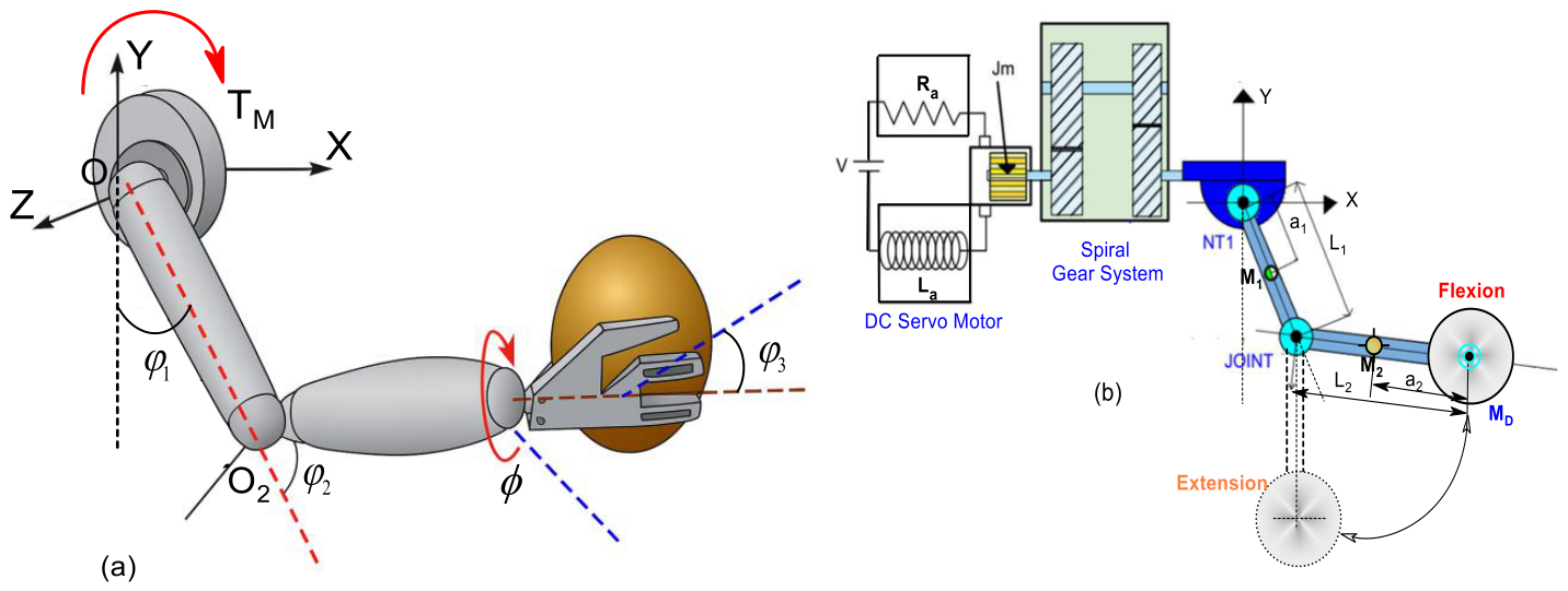
Figure 1 illustrates the complete electromechanical architecture used in this study, which is structured as a multi-degree-of-freedom (DOF) model comprising three rigid links representing the upper arm (L₁), forearm (L₂), and hand (b). There are two rotating joints: The elbow joint is modeled as a universal joint (effectively capturing torsion and flexion), with angular motion governed by parameters θ₁, θ₂, and θ₃. The wrist joint is simplified as a 1-DOF spherical joint, enabling limited rotation. Each segment has an associated mass (M₁, M₂) and moment of inertia (J₁, J₂), and the system assumes planar motion (X–Y plane). Springs and dampers simulate the elasticity and energy dissipation properties of muscles, tendons, and ligaments. These elements are used to connect the joints and absorb torsional vibrations. The torsional springs have stiffness coefficients k_t1 and k_t2, while the dampers have coefficients c_t1 and c_t2.

2.3. Dynamic Model of the Electromechanical System—DC Motor and Gear Assembly

The proposed human-inspired electromechanical arm system combines mechanical and electromechanical subsystems to investigate load-dependent dynamic behavior under external excitation. The model consists of three rigid segments representing the upper arm, forearm, and hand, connected by joints that mimic the physiological behavior of the shoulder, elbow, and wrist. The elbow is modeled as a universal joint capable of flexion and torsion, while the wrist is simplified as a one-degree-of-freedom ball-and-socket joint. Torsional springs and dampers are incorporated to simulate the elasticity and energy dissipation of muscles, tendons, and ligaments. The system is powered by a DC motor connected to a gear transmission, replicating the rotational function of the shoulder. The arm system is actuated by a DC motor coupled with a gear transmission system, modeling the shoulder joint. This motor serves as the actuator, providing rotational motion and torque. The motor is modeled using its electrical equivalent circuit, with resistance (R_a), inductance (L_a), and back electromotive force (K_b) (Figure 1b).

Control of motor torque (T_m) and angular velocity is implemented via Laplace transform formulations, resulting in transfer functions that govern system behavior. The feedback mechanism utilizes a variable controller parameter, K_b, which significantly influences system stability, enabling the modulation of the motor’s response to load changes. The complete system is modeled using nonlinear coupled differential equations based on Lagrangian mechanics, considering kinetic, potential, and dissipative energies.

2.4. Electromechanical Subsystem-Control System Components Expression

The armature speed of a DC motor is adjusted by the armature voltage $e_a(t)=i_a(t)R_a+K_b{\displaystyle \frac{d{\theta }_m}{dt}}$, Kirchhoff’s voltage law then facilitates the calculation of the total torque. The electromagnetic torque (T_m) is directly proportional to the armature current (I_a), consistent with classical DC motor theory. When expressed in the Laplace domain, the torque formulation incorporates the effect of armature inductance (L_a), which introduces dynamic behavior into the current response. The present analysis considers a gear train integrated into a robotic actuation system. The primary role of the gear assembly is to reduce the angular velocity of the load by a factor (n), thereby increasing the output torque available at the driven shaft.

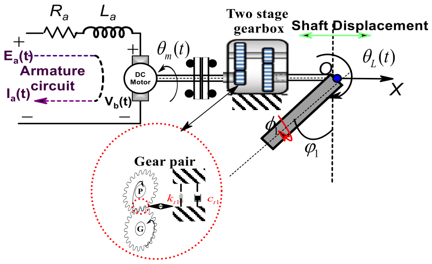
The first analysis uses gears in robotic applications to reduce the load’s angular velocity by a factor n by analyzing output parameters such as internal damping c_meq and gear inertia J_meq. For the gear train system shown in Figure 2, the relationship between the armature current $i_a(t)$, the applied voltage E_a(t), and the back EMF, V_b(t)—in a closed-loop transfer function—is calculated using unitary feedback, which gives the following transfer result in the Laplace transform [17]. The fundamental electrical relationship between the applied voltage, the armature current, and the back electromotive force (EMF) is therefore written as:

$$V_a=R_a{i}_a+L_a{\displaystyle \frac{d{i}_a}{dt}}+K_b\omega$$

(1)

The electromagnetic torque ($T_m$) is directly proportional to the armature current ($i_a$), consistent with classical DC motor theory. When expressed in the Laplace domain, the torque formulation incorporates the effect of armature inductance ($L_a$), which introduces dynamic behavior into the current response. This representation follows the standard control-system modeling approach described by Ogata [18], where the motor equations are systematically transformed into the s-domain for transfer function development. The resulting expression is given by:

$$T_m=K_t{i}_a$$

(2)

Substituting $i_a$:

$$T_m(s)={\displaystyle \frac{K_t}{R_a+L_{a}s}}\left(V_a(s)-K_b\omega (s)\right)$$

(3)

The equation indicates that the motor torque is proportional to the armature current, while its dynamic evolution is indirectly influenced by variations in motor speed via the back-EMF term. Let us first discuss the mechanical constants, J_meq and c_meq, by considering Figure 2, which shows a motor with inertia J_m and damping C_m at the armature driving a gear system with inertia J_G and damping C_G and a load consisting of inertia J_L and damping C_L. For the gear-train configuration illustrated in Figure 2, the torque equilibrium about the motor shaft ${\theta }_m$ leads to the dynamic equation summarized:

$$(J_{meq}{s}^2+c_{meq}s){\theta }_m(s)=K_t(1-L_a/R_{a}s)I_a(s)$$

(4)

This expression accounts for the reflected inertia and damping effects due to the transmission ratio. Furthermore, to establish the input motion ${\theta }_L(s)$, the overall transfer function of the electromechanical system is derived by combining Equations (1) and (3), eliminating the armature current variable, and writing the loop equation for the armature circuit in the Laplace domain. The simplified form yields:

$${\displaystyle \frac{{\theta }_L(s)}{E_a(s)}}={\displaystyle \frac{n{K}_t(\frac{s}{J_{meq}{R}_a}-\frac{1}{J_{meq}{L}_a})}{s(s^2+(\frac{R_a}{L_a}+A_a)s+B_a)}}$$

(5)

where J_meq = n²J_A + n₁²J_G + J_m, c_meq = n² C_A + n₁² C_G + c_m, and n = n₁ n₂ = (N₁N₃/N₂N₄), represent the equivalent moment of inertia, the equivalent viscous-friction coefficient referred to the motor shaft, and the overall transmission ratio of the gear train, respectively. $A_a=c_{meq}/J_{meq}+K_t{K}_b/J_{meq}{R}_a,$ and $B_a=c_{meq}{R}_a/J_{meq}{L}_a-K_t{K}_b/J_{meq}{L}_a$.

In systems analysis, applied forces are crucial to capturing intrinsic characteristics such as inertia, damping, and stiffness. Accurate predictive models can reproduce the dynamics of systems, such as the driving force of an arm, as described by:

$$F_b(t)={\displaystyle \frac{K_t{N}_g{V}_b(t)}{R_a{r}_{mg}}}-{\displaystyle \frac{K_t{N}_g{K}_b\dot{X}(t)}{R_a{r}_{mg}^2}}$$

(6)

where r_mg and N_g are, respectively, the radius of the motor pinion and the planetary gearbox ratio. Using unitary feedback, the closed-loop transfer function is thus calculated and plotted in Figure 3, which gives the following transfer function result established as:

$${\displaystyle \frac{{\theta }_L(s)}{E_a(s)}}={\displaystyle \frac{18,000s-18}{s\left(s^2+(17+K_b)s+1000-2.964K_b\right)}}$$

(7)

To represent the DC motor vibration and input arm function, the study selects a representative set of DC motor property values defined in

Table 1. Physical parameters of the DC motor [11,19].

DC Coupled Motor-Gearbox	Value and Unit
Motor rotor inertia (Jmeq)	0.00025 kg·m2
DC Motor’s input shaft inertia (Jm)	0.0005 kg·m2
Motor viscous damping coefficient (cmeq)	0.00015 Nms/rad
Torsional damping coefficient (ct)	0.8 Nms/rad
Load viscous damping coefficient (cm)	0.00015 Nm/rad/s
Torsional stiffness of flexible joint (Kt)	1.08 Nm/rad
Motor torque constant (Kt)	150 Nm/Amp
Armature resistance (Ra)	2 Ω
Armature inductance (La)	0.003 H
Gear pair ratio (n)	0.2
Effective radius (rmg)	0.02
Gearbox efficiency ($N$g)	1
Back-EMF constant (Kb)	Adjustable (V-s/rad)

. The parameters presented in Table 1 and

Table 2. Physical Parameters and Model Assumptions [11,19].

Parameter Description	Value and Unit
Upper-arm mass (M1)	0.0725 kg
Forearm mass(M2)	0.125 kg
Hand mass 1 (Mhg1)	1.17 kg
Hand mass 2 (Mhg2)	0.178 kg
Motor mass (Mm)	10.57 kg
External load mass (MD)	Adjustable kg
Torsional stiffness of L1 (kτ1)	5 × 105 Nm/rad
Torsional stiffness L2 (kτ2)	5 × 105 Nm/rad
Joint 1 translational stiffness (kt1)	6 × 104 N/m
Joint 2 translational stiffness (kt2)	6 × 104 N/m
Joint 1 torsional viscous damping(cτ1)	0.0025 Nms/rad
Joint 2 torsional damping (cτ2)	0.005 Nms/rad
Upper-arm joint inertia (Jb1)	0.082 kg·m2
Lower-arm joint inertia (Jb2)	0.082 kg·m2
Length arms (L1 & L2)	0.32 m
Up & down length arms (a1 & a2)	0.18 m
Length of hand (b)	0.2 m

were chosen to reflect representative values established in previous studies on electromechanical actuation systems and dynamic upper-limb models [11,19].

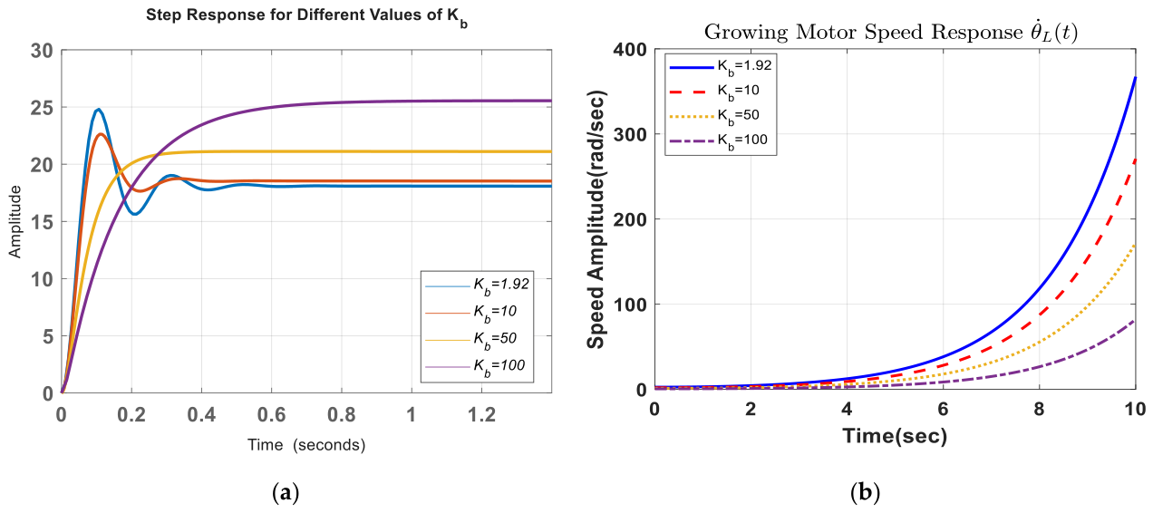
Discussion 1: An analysis of Figure 3 revealed that as K_b increases (up to 100), the response becomes more attenuated, the oscillations gradually disappear, and the stability of the system improves significantly. Since this study focuses on nonlinear stability and bifurcation behavior under external load, the transient response shown in Figure 3a is not used here for classical controller performance tuning based on rise time, settlement time, or overshoot. It serves, rather, to illustrate the influence of the back electromotive force coefficient (K_b) on the attenuation of oscillations and the tendency towards overall stability of the electromechanical subsystem. A parametric sensitivity analysis identified a critical electromechanical feedback threshold at approximately K_b = 1.92, where the first self-sustaining oscillations and the beginning of limit cycle behavior appear, marking a qualitative change in the system dynamics. This demonstrates that K_b acts as an effective control parameter to regulate energy dissipation and reduce unwanted vibrations. The results indicate that higher K_b values increase vibration attenuation and improve overall dynamic stability. Within the range studied, values between 50 and 100 offer the most stable response. This parameter thus becomes essential to optimize vibrational comfort and prevent resonance.

2.5. Joint Disturbance Function and Behaviour

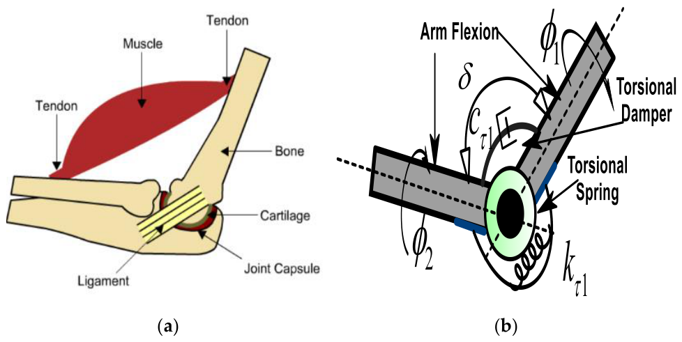
Inspired by the structure of the human elbow, and more specifically, the humeroulnar joint, a one-degree-of-freedom (DOF) Cardan joint was developed in a recent study [11], as illustrated in Figure 4a.

This joint will be adopted in the present work. The analysis involves moving the input arm into flexion and extension and measuring the resulting deformation as a function of the rotation angle δ of the coupling joint, as shown in Figure 4b. The model shown in Figure 4b incorporates both a torsion spring and a shock absorber, effectively reproducing arm flexion and extension through variations in the joint angle. To simulate different arm postures, the joint angle is assumed to be relatively large, typically 30 degrees or more, which amplifies the model’s nonlinearity. This study uses the relationship between the upper and lower arms as a perturbation parameter, modeled using Cardan joint kinematics [17]. To capture the nonlinearities mentioned, the relationship between the upstream motion and the downstream motion ${\varphi }_2\left(t\right)$ can be defined as:

$${\varphi }_2(t)={\varphi }_1(t)+\xi {\varphi }_1(t)={\varphi }_1(t)(1+\xi (t))$$

(8)

where ξ(t) ≠ 0 the dimensionless parameter that represents the aggregate perturbation. Depending on the physical source of the distortion, it can be further decomposed. Applying the tangent trigonometric function after appropriate manipulation.

$$\tan ({\varphi }_1(t)\xi (t))={\displaystyle \frac{(1+\cos \delta (t))\tan {\varphi }_1(t)}{(\cos \delta (t){\tan }^2{\varphi }_1(t)+1)}}$$

(9)

Solving this equation for ξ(t), the model of a flexible articulated arm manipulator is defined as follows:

$$\xi ({\varphi }_1)=\left\{\begin{array}{l}0\\ {\displaystyle \frac{1}{{\varphi }_1}}{\tan }^{-1}\left({\displaystyle \frac{(1+\cos \delta )\tan {\varphi }_1}{(\cos \delta {\tan }^2{\varphi }_1+1)}}\right)\end{array}\right.$$

(10)

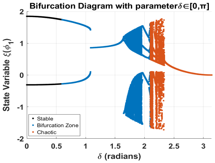
The illustration of the evolution of state ξ(${\varphi }_1$) as a function of joint angle δ ∈ [0, π], revealing dynamic transitions typical of nonlinear systems, is presented in Figure 5 below.

Discussion 2: Figure 5 indicates that for small misalignment angles ($\delta \approx 0–$0.6 rad), the system converges to a stable fixed point. As $\delta$ increases to about 0.6–1.2 rad, periodic oscillations emerge, marking a transition to limit-cycle behavior. A further increase ($\delta \approx$ 1.2–2 rad) produces successive period-doubling bifurcations, while for $\delta >2.1$ rad the response exhibits characteristics associated with chaotic dynamics. These results reveal a progressive transition from stable equilibrium to periodic oscillations, period-doubling bifurcations, and ultimately chaotic behavior, highlighting critical angular zones. Operation within this area may lead to unpredictable dynamic responses and should be avoided in practical electromechanical and robotic arm design.

2.6. Formulation of Equations of Motion

The proposed electromechanical model presented in Figure 1 comprises three discrete masses, shock absorbers, and springs. The developed mathematical model assumes that rotational inertia is neglected and that the composite mass of each rod is concentrated at its center of gravity. For simplicity, the proposed model assumes ideal kinematic conditions, neglecting joint misalignment, assembly tolerances, encoder uncertainties, backlash, and transmission errors. Consequently, the study focuses on nonlinear dynamic stability and bifurcation behavior rather than geometric error propagation or positioning accuracy. It also assumes that the upper and lower rods have significant angular misalignment due to the coupling of a single U-joint to maintain the torsional motion of the rods and preserve the nonlinear coupling effects, as shown in Figure 1b.

To define the total energy of the arm–disc system, the center of inertia of each rod and the hinges are first determined, with the upper and lower rods representing arms 1, 2, and 3, respectively, in the Cartesian plane, based on the geometry shown in Figure 1 and the overall coordinates of the arms. The following equations can be derived:

$${\overrightarrow{CG}}_1=\left\{\begin{array}{l}{x}_{CG1}(t)=X(t)-a_1\sin {\phi }_1(t)\\ y_{CG1}(t)=-a_1\cos {\phi }_1(t)\end{array}\right.$$

(11)

$${\overrightarrow{CG}}_2=\left\{\begin{array}{l}{x}_{CG2}(t)=X(t)-a_2\sin ({\phi }_1(t)-{\phi }_2(t))-L_1\sin {\phi }_1(t)\\ y_{CG2}(t)=-a_2\cos ({\phi }_1(t)-{\phi }_2(t))-L_1\cos {\phi }_1(t)\end{array}\right.$$

(12)

The center of gravity of the mass of bonds 1 to 3 can be expressed as:

$${\overrightarrow{CG}}_{h{g}_1}=\left\{\begin{array}{l}{x}_{Gh{g}_1}(t)=X(t)-L_1\sin {\phi }_1(t)\\ y_{Gh{g}_1}(t)=-L_1\cos {\phi }_1(t)\end{array}\right.$$

(13)

$${\overrightarrow{CG}}_{h{g}_2}=\left\{\begin{array}{l}{x}_{Gh{g}_2}(t)=X(t)+b\cos {\phi }_3(t)-L_2\cos {\phi }_2(t)\\ y_{Gh{g}_2}(t)=b\sin {\phi }_3(t)\end{array}\right.$$

(14)

Taking into account the angular displacements of each link, the torsional angle, and the lumped mass of the links, the total energy of a system is the sum of kinetic energy, potential energy, and dissipation energy due to contact damping, which can be obtained based on Lagrange’s law. The equations governing the system were established using the Euler–Lagrange formalism applied to the configuration of the electromechanical arm illustrated in Figure 1, while the standard relations of the motor and the rigid body were taken from the literature. The kinetic energy of the arm’s system can be obtained as:

$$\begin{array}{l}{T}_{Total}={\displaystyle \frac{1}{2}}\left(J_{b1}+J_D+M_1{a}_1^2+M_2{a}_2^2+M_{hg}{L}_1^2+M_2{L}_1^2\right){\dot{\phi }}_1{(t)}^2+M_2{L}_1{a}_2\cos ({\phi }_2(t)){\dot{\phi }}_1{(t)}^2\\ +{\displaystyle \frac{1}{2}}\left(J_{b1}+J_{b2}\Gamma {(t)}^2\right){\dot{\varphi }}_1{(t)}^2+{\displaystyle \frac{1}{2}}\left(M_1+M_2+M_{hg}+M_{hg2}+M_m+{\displaystyle \frac{J_m{N}_g^2}{r_{mg}^2}}\right)\dot{X}{(t)}^2\end{array}$$

$$\begin{array}{l}+{\displaystyle \frac{1}{2}}\left(J_{b2}+J_D+M_2{a}_2^2+M_{hg2}{L}_2^2\sin ({\phi }_2(t))\right){\dot{\phi }}_2{(t)}^2+{\displaystyle \frac{M_{hg2}{b}^2}{2}}{\dot{\phi }}_3{(t)}^2\\ -M_2{a}_2(a_2+L_1\cos ({\phi }_2(t))){\dot{\phi }}_2(t){\dot{\phi }}_1(t)+\left(M_2{a}_2\cos \left({\phi }_2(t)-{\phi }_1(t)\right)+M_{hg2}{L}_2\sin ({\phi }_2(t))\right){\dot{\phi }}_2(t)\dot{X}(t)\\ \hspace{1em}\hspace{1em}-M_2{a}_2\cos \left({\phi }_2(t)-{\phi }_1(t)\right){\dot{\phi }}_1(t)\dot{X}(t)-M_{hg2}b\sin ({\phi }_3(t)){\dot{\phi }}_3(t)\dot{X}(t)\\ \hspace{1em}\hspace{1em}\left(M_2{L}_1+M_{hg}{L}_1+M_1{a}_1\right)\cos {\phi }_1(t){\dot{\phi }}_1(t)\dot{X}(t)-M_{hg2}{L}_{2}b\sin ({\phi }_3(t))\sin ({\phi }_2(t)){\dot{\phi }}_3(t){\dot{\phi }}_2(t)\end{array}$$

(15)

Based upon the displacement vector of the connected links, the potential energy of the arms system can be written as:

$$\begin{array}{l}{V}_T={\displaystyle \frac{1}{2}}{k}_{t2}{\left({\phi }_2(t)-{\phi }_1(t)\right)}^2+{\displaystyle \frac{1}{2}}{k}_{\tau 1}{\left(\epsilon (t)\right)}^2+{\displaystyle \frac{1}{2}}{k}_{\tau 2}{\left({\phi }_3(t)-{\phi }_2(t)\right)}^2+{\displaystyle \frac{1}{2}}{k}_{t1}X{(t)}^2\\ +M_{2}g{a}_2\cos ({\phi }_2(t)-{\phi }_1(t))+(M_{1}g{a}_1+M_{hg}g{L}_1+M_{2}g{L}_1)\cos {\phi }_1(t)\end{array}$$

(16)

Hence, the total dissipated energy introduced by the relative motion of the joint obeys:

$$R_T={\displaystyle \frac{1}{2}}{c}_{t1}\dot{X}{(t)}^2+{\displaystyle \frac{1}{2}}{c}_{\tau 1}{\left[(1-\Gamma (t)){\dot{\varphi }}_1(t)\right]}^2+{\displaystyle \frac{1}{2}}{c}_{t2}{\left({\dot{\phi }}_2(t)-{\dot{\phi }}_1(t)\right)}^2+{\displaystyle \frac{1}{2}}{c}_{\tau 2}{\left({\dot{\phi }}_3(t)-{\dot{\phi }}_2(t)\right)}^2$$

(17)

Applying Lagrange’s equation to the total kinetic, potential, and dissipative energies produces a set of coupled nonlinear differential equations that describe the rotational dynamics of three-armed segments. The resulting system contains cubic and cross-coupling terms capable of generating complex nonlinear phenomena, including bifurcations and chaotic responses under specific operating conditions. Using Lagrange’s equation for a set of independent generalized coordinates $X,{\phi }_1,{\varphi }_1,{\phi }_2$ and ${\phi }_3$ rearranging the movement of the arms follows a nonlinear behavior, as follows:

For the first generalized coordinate X, ${\displaystyle \frac{d}{dt}}({\displaystyle \frac{\partial T_{Total}}{\partial \dot{X}}})-{\displaystyle \frac{\partial T_{Total}}{\partial X}}+{\displaystyle \frac{\partial V_T}{\partial X}}+{\displaystyle \frac{\partial R_T}{\partial \dot{X}}}=0$

$$\begin{array}{l}(M_1+M_2+M_{hg}+M_{hg2}+M_m+{\displaystyle \frac{J_m{N}_g^2}{r_{mg}^2}})\ddot{X}(t)-((M_1{a}_1+M_2{L}_1+M_{hg}{L}_1)\cos {\phi }_1\\ +M_2{a}_2\cos ({\phi }_2-{\phi }_1)){\ddot{\phi }}_1(t)+\left(M_2{a}_2\cos ({\phi }_2(t)-{\phi }_1(t))+M_{hg2}{L}_2\sin ({\phi }_2(t))\right){\ddot{\phi }}_2(t)\\ -M_{hg2}b\sin {\phi }_3(t){\ddot{\phi }}_3(t)+c_{t1}\dot{X}+k_{t1}X=V_{cX}(t)\end{array}$$

(18)

Following the same manipulation for each first generalized coordinate ${\phi }_1,{\varphi }_1,{\phi }_2$ and ${\phi }_3$, the equations are obtained as:

$$\begin{array}{l}-\left((M_2{L}_1+M_{hg}{L}_1+M_1{a}_1)\cos {\phi }_1(t)\right)\ddot{X}(t)+\left(J_D+J_{b1}+M_1{a}_1^2+M_2{a}_2^2+M_2{L}_1^2+M_{hg}{L}_1^2\right){\ddot{\phi }}_1(t)\\ +2L_1{M}_2{a}_2\cos ({\phi }_2){\ddot{\phi }}_1(t)+M_2{a}_2\cos ({\phi }_2-{\phi }_1)\ddot{X}(t)-M_2{a}_2\left(a_2+L_1\cos ({\phi }_2(t))\right){\ddot{\phi }}_2(t)\\ +c_{t2}({\dot{\phi }}_1(t)-{\dot{\phi }}_2(t))+k_{t2}({\phi }_1(t)-{\phi }_2(t))=V_{c{\phi }_1}(t)\end{array}$$

(19)

$$\left(J_{b1}+J_{b2}{{\Gamma }_1}^2\right){\ddot{\varphi }}_1(t)+{\displaystyle \frac{c_{\tau 1}{\Gamma }_3}{{{\Gamma }_2}^2}}{\dot{\varphi }}_1(t)-{\displaystyle \frac{k_{\tau 1}{\Gamma }_3\epsilon }{{\Gamma }_2}}{\varphi }_1(t)=V_{c{\varphi }_1}(t)$$

(20)

$$\begin{array}{l}\left(M_{hg2}{L}_2\sin ({\phi }_2(t))+M_2{a}_2\cos \left({\phi }_2-{\phi }_1\right)\right)\ddot{X}(t)-\left(M_2{a}_2(a_2+L_1\cos ({\phi }_2(t))\right){\ddot{\phi }}_1(t)\\ +\left(J_D+J_{b2}+M_2{a}_2^2+M_{hg2}{L}_2^2\sin {({\phi }_2(t))}^2\right){\ddot{\phi }}_2(t)-M_{hg2}{L}_{2}b\sin {\phi }_3(t)\sin ({\phi }_2(t)){\ddot{\phi }}_3(t)\\ +c_{t2}({\dot{\phi }}_2(t)-{\dot{\phi }}_1(t))+c_{\tau 2}({\dot{\phi }}_2(t)-{\dot{\phi }}_3(t))+k_{t2}({\phi }_2(t)-{\phi }_1(t))+k_{\tau 2}({\phi }_2(t)-{\phi }_3(t))=V_{c{\phi }_2}(t)\end{array}$$

(21)

$$\begin{array}{l}-M_{hg2}b\sin ({\phi }_3(t))\ddot{X}(t)+M_{hg2}{b}^2{\ddot{\phi }}_3(t)-M_{hg2}{L}_{2}b\sin ({\phi }_3(t))\sin ({\phi }_2(t)){\ddot{\phi }}_2(t)\\ +c_{\tau 2}({\dot{\phi }}_3(t)-{\dot{\phi }}_2(t))+k_{\tau 2}({\phi }_3(t)-{\phi }_2(t))=V_{c{\phi }_3}(t)\end{array}$$

(22)

In the present paper, the authors have written the equation of motion directly. However, the derivation of the equation of motion and the specific expressions for these generalized vector terms have been explained in detail in [11].

2.7. Numerical Integration and Resolution Methods

In this section, numerical simulations are conducted based on the established model of an electromechanical system. The Newmark method is employed to capture dynamic responses with a time step of 2π/512. It is important to note that the mass matrix of the whole system varies with time due to the piecewise linear angular displacement of the arm joint. Moreover, the stiffness matrix, damping matrix, and external force vector require continuous updating during numerical integrations based on rotational speed and vibration displacement. The updating process of the model, along with numerical iteration and computational procedures, is further illustrated. The stability of the torsional vibration is evaluated using bifurcation diagrams, Poincaré maps, and the largest Lyapunov Exponent. The physical parameters of the arm system were selected to ensure physically realistic joint behavior and dynamic responses within the range reported in previous studies on electromechanical and robotic arms [11,19]. The values were selected to represent a generic electromechanical arm system and were used primarily to study nonlinear stability trends rather than to reproduce the exact biomechanical behavior of a specific human-inspired electromechanical arm subject.

3. Results and Discussion

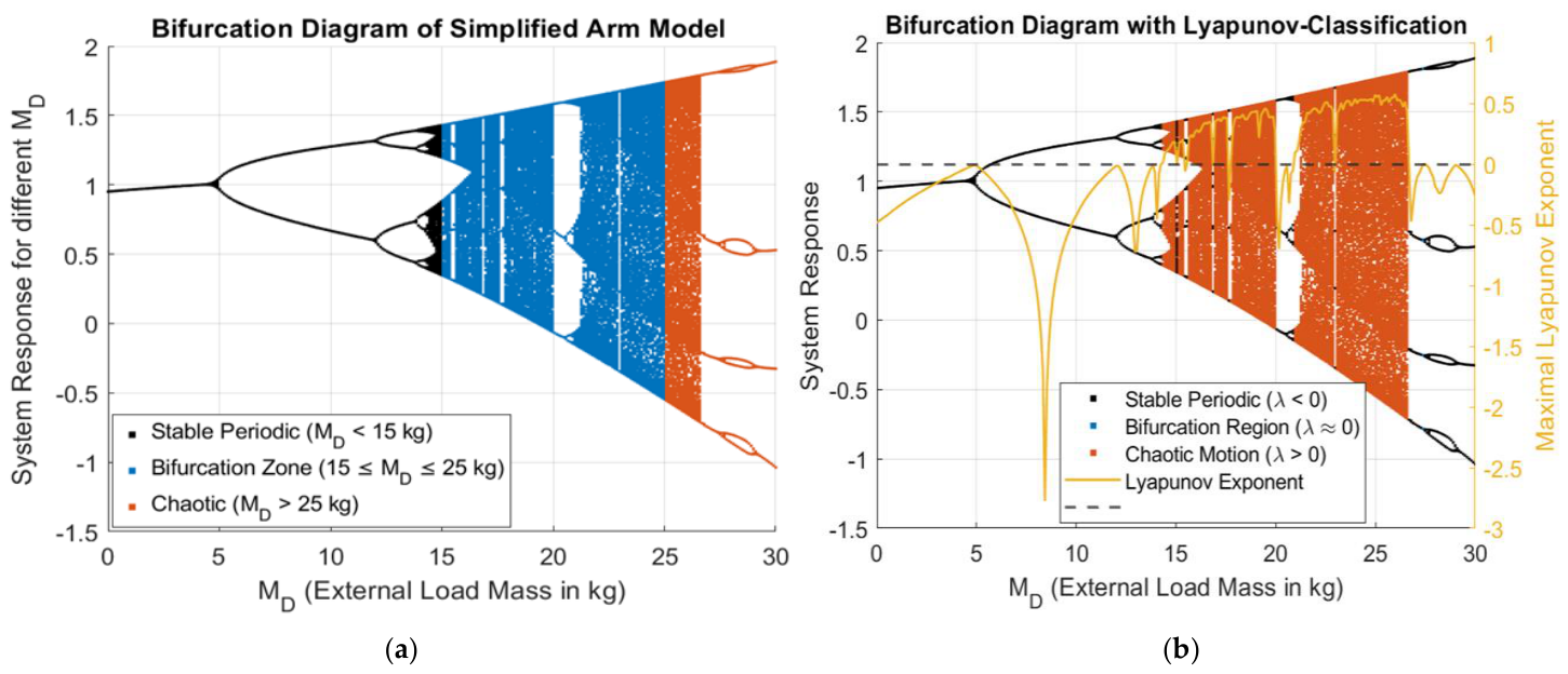
Numerical simulations were performed after eliminating transient effects to ensure that only the steady-state response was analyzed. The physical properties of the arm–shoulder are listed in Table 2. For the numerical method, the initial conditions and step sizes are chosen to ensure an accurate yet computationally inexpensive solution. Figure 6 and

Table 3. Arm overview to ensure predictable behavior.

Range MD (kg)	Observed Dynamics	Lyapunov Exponent	Dynamic Behavior
MD < 15	Stable (Fixed point)	λ < 0	Periodic
15 ≤ MD < 25	Onset of Instability	λ ≈ 0	Quasi-Periodic
25 ≤ MD < 35	Nascent chaotic regime	λ > 0	Weak Chaos
MD ≥ 35	Fully developed chaos	λ ≫ 0	Strong Chaos

reveal that small external loads produce stable periodic responses, while increasing loads gradually destabilize the system through successive bifurcations. When the external load exceeds approximately 15 kg, quasi-periodic oscillations appear, followed by period-doubling bifurcations and eventual chaotic behavior. Therefore, the system does not exhibit a single low-load regime but rather a succession of nonlinear dynamic transitions as the load increases.

Discussion 3: The interpretation of the bifurcation diagram in Figure 6a reveals three distinct zones depending on the value of the added mass M_D. In the stable zone (M_D < 15 kg), represented by black dots, the system exhibits regular periodic behavior with convergence towards a fixed orbit. The Lyapunov exponent is strictly negative, indicating asymptotic stability and effective damping of perturbations. When M_D reaches a value between 15 and 25 kg, we enter a bifurcation zone (blue dots), marked by the appearance of limit cycles and period-doubling phenomena (2, 4, etc.). This transition is characteristic in Figure 6b of a periodic bifurcation, where the Lyapunov exponent becomes zero or slightly positive, signaling increased sensitivity to initial conditions and the appearance of quasi-periodic or pre-chaotic dynamics (Figure 6b). Finally, for M_D > 25 kg, the system enters a chaotic zone (grey dots), where the diagram reveals a dense cloud of points indicating a very unstable and unpredictable response. In this region, the largest Lyapunov exponent becomes positive, indicating an exponential divergence of neighboring trajectories and providing strong evidence for deterministic chaos. This region should be avoided in mechanical or electromechanical applications, as it represents a loss of regularity and control of the system. As outlined in Table 3, the critical load threshold was identified at approximately M_D = 35 kg, where the largest Lyapunov exponent becomes significantly positive, and the bifurcation structure evolves towards a dense chaotic attractor. This threshold marks the transition from weakly chaotic dynamics to a fully developed chaotic regime.

This dynamic division is fundamental to identifying functional safety zones and anticipating unstable regimes to be avoided in electromechanical or robotic design.

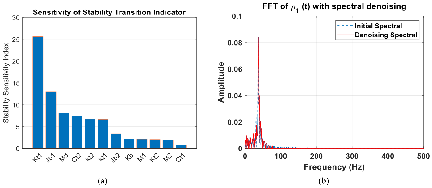
To determine which parameters are most critical for the stability of the proposed system, a local sensitivity analysis was conducted with reference to nominal operating conditions. Figure 7a shows the calculated stability sensitivity index for the model’s principal parameters. The findings demonstrate that torsional stiffness K_t1 is the most significant factor, followed by the moment of inertia J_b1 and the external load M_D. The influence of damping coefficients and the masses of the various segments is secondary, while the back electromotive force coefficient K_b plays a role in the system’s stability, although its sensitivity is lower within the range of parameters considered. These findings show that the bifurcation phenomena and stability transitions detected in this study largely result from the relationship between joint stiffness, inertial effects, and the imposed load. Therefore, K_t1 and J_b1 primarily affect the amplitude of the response, while M_D and K_b influence the stability limit of the system.

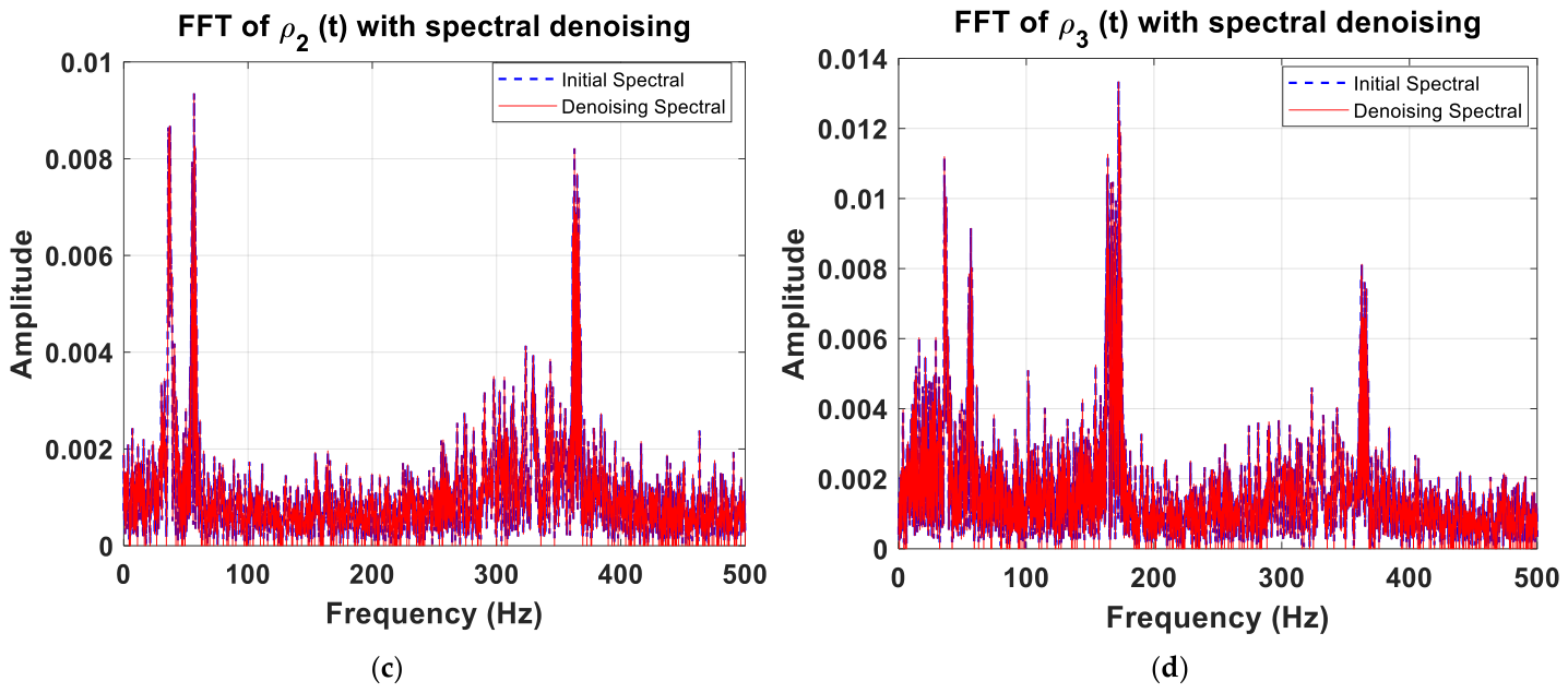
In an electromechanical analog system such as the human-inspired electromechanical arm, Figure 7b–d show the FFT spectra of the generalized coordinates ρ₁, ρ₂, and ρ₃. For low loads, the vibrational energy is concentrated around a limited number of dominant frequencies, reflecting a stable dynamic behavior. The spectra highlight the distribution of the system’s vibrational energy in the frequency domain and allow the identification of the dominant dynamic components associated with the different degrees of freedom. Each coordinate exhibits characteristic frequencies corresponding to the dynamic modes of the coupled electromechanical system. Signal ρ₃ (Figure 7d), associated with a deep arm torsion angle, shows the highest frequency. This angle is subject to greater dynamic influence due to increased inertial coupling and proximity to the maximum loading zone. In contrast, the responses associated with ρ₁ and ρ₂ (Figure 7b,c) remain mainly concentrated around their respective dominant frequencies. As the external load is not yet considered, inertial coupling and nonlinear joint interactions amplify the high-frequency content of the response, especially along the ρ₃ coordinate.

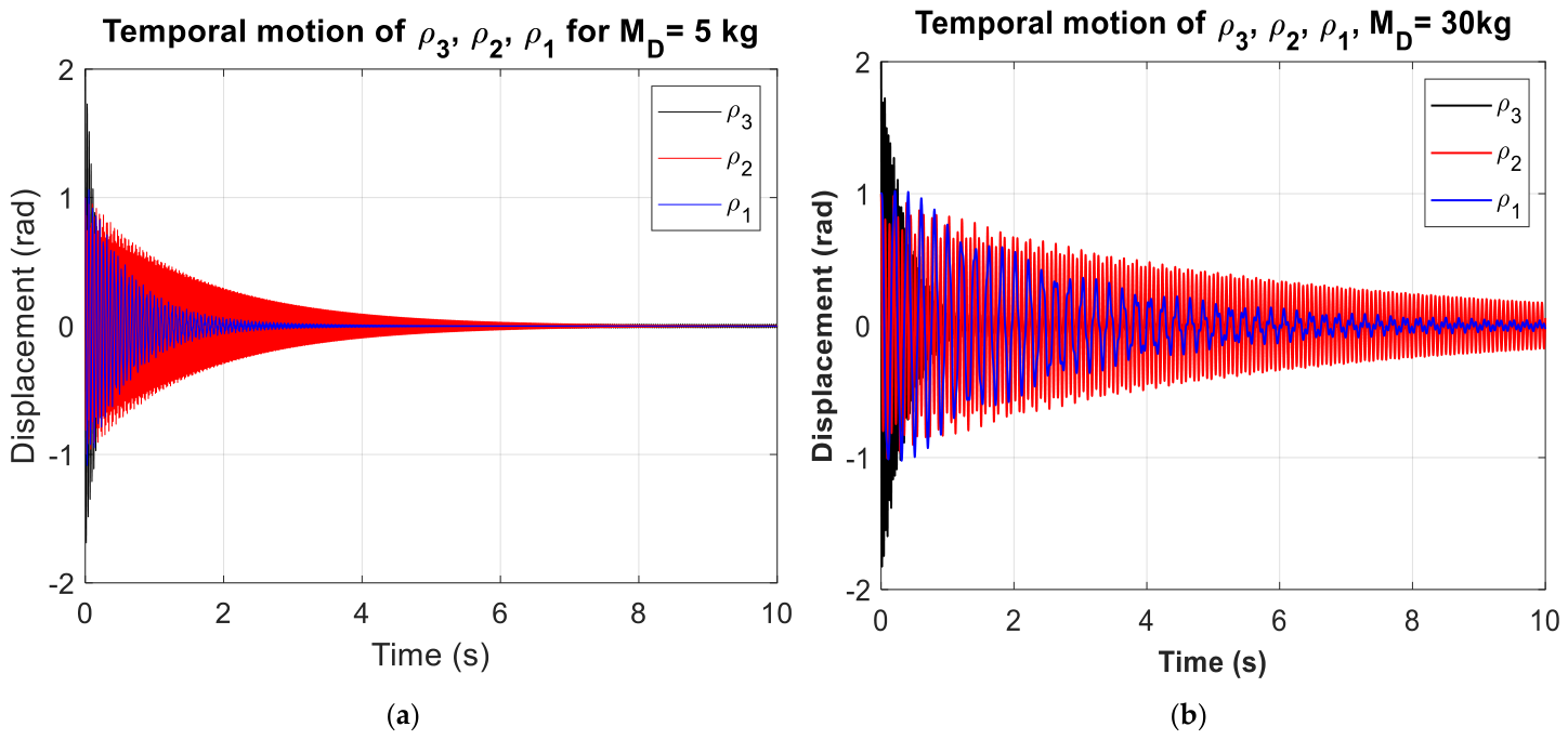
Figure 8 shows the time evolution of the coordinates ρ₁, ρ_2, and ρ₃ under two loading conditions. At low load, M_D = 5 kg, the system is dynamically stable and exhibits regular and bounded oscillations of constant amplitude. At high load, M_D = 30 kg, the increased nonlinear coupling induces larger amplitudes, irregular trajectories, and reduced stability. Comparing the two load conditions reveals that larger external loads significantly alter the amplitude and kinematic complexity of the arm movement. This contrast demonstrates that higher external loads cause the system to shift from a stable periodic motion to a complex, potentially chaotic dynamic, thus validating bifurcation, FFT, and Lyapunov analyses.

Discussion 4: Figure 7 and Figure 8 provide additional information regarding the dynamic behavior of the proposed electromechanical arm system, both in the frequency and time domains. The FFT spectra displayed in Figure 7 show that the energy vibration is distributed among several dominant frequencies associated with the main dynamic modes of the coupled electromechanical system. The presence of several harmonic components confirms that the system’s response cannot be described by purely harmonic motion and reflects the influence of nonlinear stiffness and damping mechanisms. The corresponding time histories shown in Figure 8 reveal that, under low external loads, the generalized coordinates remain bounded and exhibit regular oscillatory behavior characteristic of a stable dynamic regime. As the external load (M_D) increases, the oscillation amplitudes grow, and the responses become progressively more irregular, especially for (ρ₃), indicating stronger nonlinear interactions and a progressive degradation of system stability. These observations are consistent with bifurcation diagrams and Lyapunov exponent analysis, which collectively indicate a transition from stable periodic motion to increasingly complex nonlinear dynamics as the charge level approaches the critical threshold.

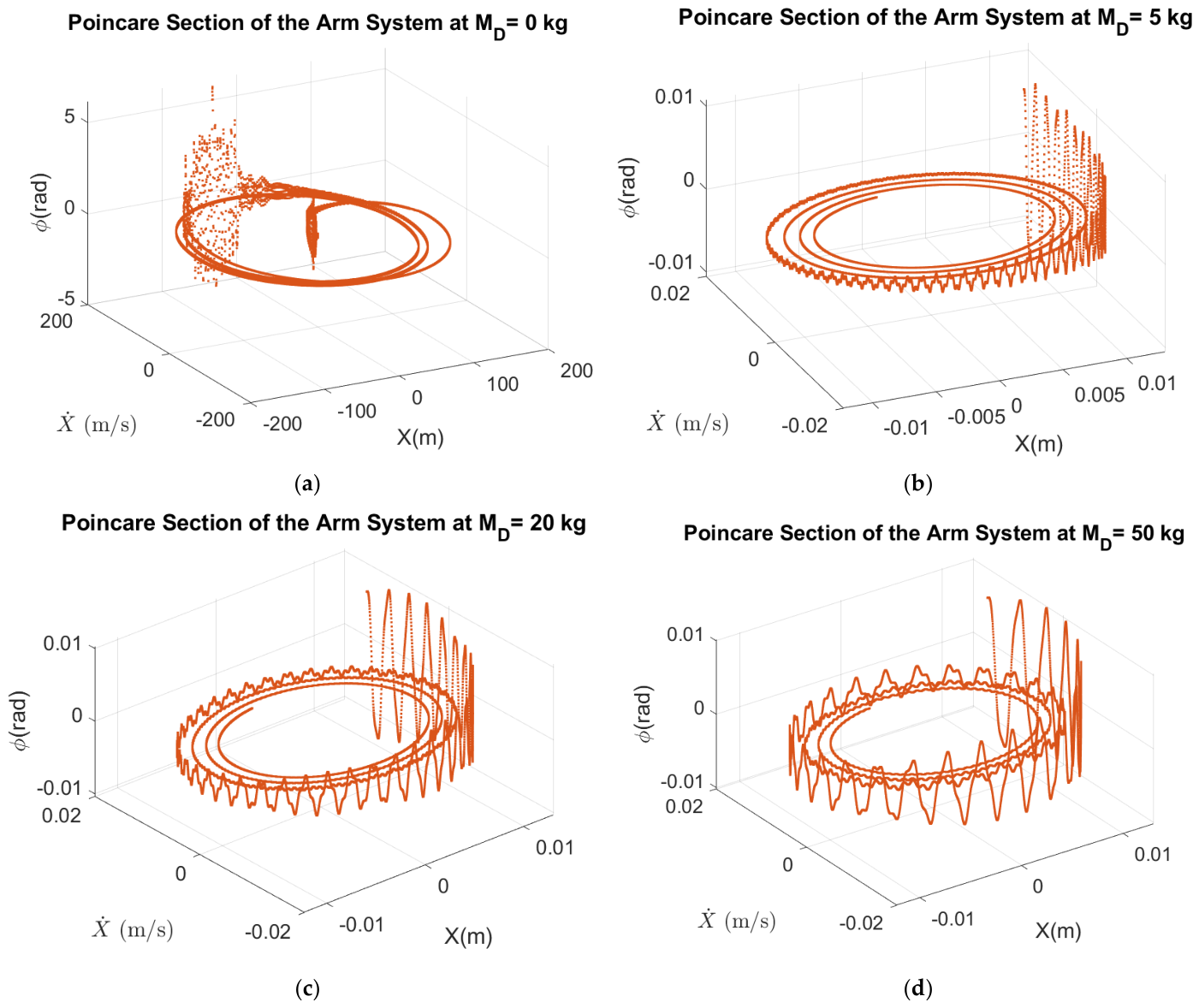
In this study, in addition to classical frequency methods such as FFT, the Poincaré method makes it possible to directly visualize the impact of the increase in mass M_D on the dynamic stability of the human-inspired electromechanical arm system by highlighting the progressive transition from regular movements to chaotic behavior through different bifurcation stages, as shown in Figure 9.

Discussion 5: Poincaré maps in Figure 9a–d illustrate the dynamic evolution of the human-inspired electromechanical arm system under different M_D masses. Points cluster at M_D = 0 kg and 5 kg, forming closed or quasi-closed trajectories that indicate stable, highly damped periodic behavior. At M_D = 20 kg, the point structure begins to disperse, suggesting the onset of quasi-periodic regimes where multiple frequencies interact. At an exaggerated value, M_D = 50 kg, the Poincaré section exhibits a dispersed distribution of points rather than a closed orbit, indicating a loss of periodicity and the emergence of chaotic dynamics. The dynamic behavior of the human-inspired electromechanical arm system becomes unpredictable and extremely sensitive to initial conditions. These observations show that the higher the mass carried, the lower the stability, with a gradual transition from stable periodic behavior to chaos. In a vibrating system such as a human-inspired electromechanical arm system carrying varying masses, the equations of motion quickly become nonlinear and complex to analyze directly. The progressive increase in M_D mass leads to an evolution of dynamic behavior: from a stable periodic regime for low loads (0 to 5 kg), to a quasi-periodic regime for intermediate loads (20 kg), then to chaotic behavior for heavier loads (50 kg). Cross-analysis of the combined interpretation of bifurcation diagrams, Lyapunov exponents, Poincaré maps, and FFT spectra confirmed the transition from stable periodic motion to chaotic behavior. The bifurcation diagrams revealed successive period-doubling sequences, while the Lyapunov exponents became positive in the chaotic regime, indicating exponential divergence of neighboring trajectories. The Poincaré sections evolved from closed periodic trajectories to scattered point clouds. Simultaneously, FFT spectra exhibited spectral broadening with multiple harmonics. The concordance among these independent nonlinear analysis tools constitutes strong evidence of the emergence of deterministic chaos under strong constraints. This work shows that the mass carried strongly influences the arm’s dynamics, making advanced analytical methods essential for detecting bifurcations, anticipating instabilities, and ensuring the safety of an electromechanical analog system.

4. Conclusions

This study developed a nonlinear electromechanical model inspired by the human-inspired electromechanical arm system to analyze how external loads affect the system’s dynamic stability. This simplified model neglects the complexity of muscular, tendinous, and neuromuscular dynamics to focus on dominant structural and electromechanical characteristics. This abstraction ensures computational efficiency while allowing the impact of external loads and feedback on the overall dynamic response to be assessed. The study, therefore, proposes a theoretical evaluation of the nonlinear dynamics of an electromechanical arm using numerical simulations rather than human physiological models. The preliminary results showed that the electromotive force feedback coefficient K_b plays a crucial role in vibration damping and stability control, with a critical value near K_b = 1.92 marking the onset of the first limit cycles. The numerical analysis also revealed that the external load (M_D) acts as a bifurcation parameter. As the load increases, the system gradually evolves from a stable regime to quasi-periodic behavior and then to chaos. This transition was confirmed by bifurcation diagrams, Poincaré maps, FFT spectra, and Lyapunov exponents, which reveal a progressive loss of stability under high loads.

The results help identify safe operating ranges and critical thresholds to avoid during the design and control of articulated electromechanical systems. Although the model’s mathematical structure is similar to formulations used in milling vibration analysis, its application to biomechanical and robotic systems is an original contribution. The proposed model thus provides a simplified yet relevant framework for studying the stability of robotic arms, rehabilitation devices, and human–robot interaction systems under variable loads. Future experimental validation of the proposed model, based on numerical simulations, will use a laboratory-scale electromechanical arm system. It will be equipped with a dual-encoder configuration, which can be implemented at the main joints, with one encoder mounted on the engine side and another on the transmission output side. This configuration will allow us to quantify transmission error, joint compliance, play effects, and measurement uncertainty, thus improving the accuracy of model validation.