Nonlinear Analysis for Non-Newtonian Nanofluid Flow over a Shrinking Plate with Convective Boundary Conditions

Abstract

Significance: This study addresses critical industrial and biomedical applications including glass blowing (thermal management of shrinking sheets), polymer sheet extrusion (controlled cooling), magnetic drug delivery (nanoparticle targeting), and nuclear reactor cooling (enhanced heat transfer). Aim: We present a novel nonlinear analysis of magnetohydrodynamic (MHD) boundary layer flow of a Jeffery Al₂O₃ nanofluid over a shrinking permeable plate with convective boundary conditions, uniquely integrating mixed convection, Ohmic dissipation, heat generation, Brownian motion, and thermophoresis within a non-Newtonian nanofluid framework. Methodology: The governing partial differential equations are transformed using similarity transformations and solved via the Adomian decomposition method (ADM). Comprehensive validation against RK4, RK45, and bvp4c demonstrates excellent agreement with maximum relative errors below $5\times {10}^{-4}$. Key Contribution: (i) Normal velocity decreases by 15–25% as the Biot number increases from $Bi=0.4$ to $0.6$; (ii) tangential velocity decreases by 20–30% as the magnetic parameter increases from $M=5$ to 15; (iii) temperature increases by 30–40% as the Eckert number increases from $Ec=0.5$ to $2.5$; (iv) ADM converges within 12–15 terms with $L_2$ errors $<{10}^{-5}$; (v) skin friction coefficient increases from $C_f=3.02713$ to $3.90082$ as $Q_0$ increases from 1 to 4; (vi) Nusselt number values: $Nu/\sqrt{Re}=0.4621$ at $Pr=0.7$, $0.8954$ at $Pr=2$, $3.2890$ at $Pr=20$. These quantitative findings provide design guidelines for engineers in thermal management and biomedical applications.

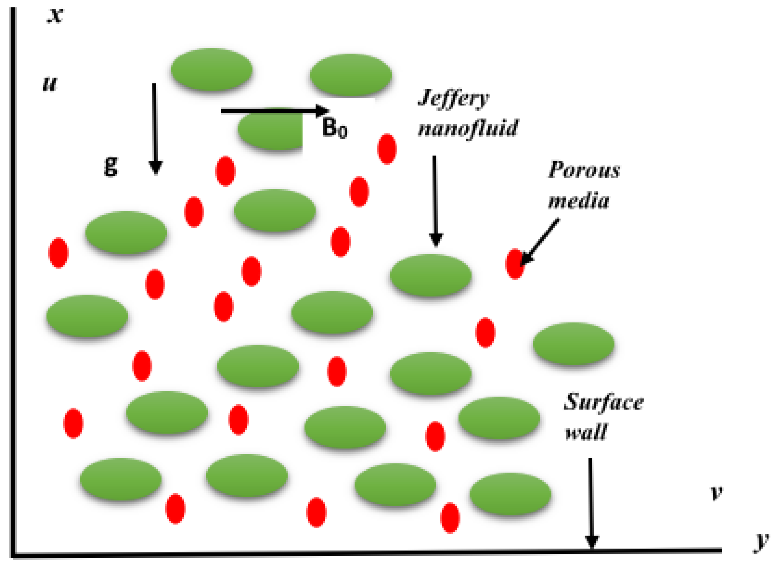
1. Introduction

1.1. Convective Boundary Conditions

When a surface is exposed to convective heat transfer obeying Newton’s cooling law, a convective boundary condition develops within the boundary layer. Unlike constant temperature boundary conditions where the surface temperature is prescribed, under convective boundary conditions the surface temperature is unknown and emerges from the thermal balance between conduction in the fluid and convection from the hot fluid. The prescribed quantities are the hot fluid temperature $T_f$ and the heat transfer coefficient $h_f$, while the surface temperature $T\left(0\right)$ is determined as part of the solution. This phenomenon is crucial in heat exchangers, drying processes, thermal management systems, and many industrial applications where surfaces interact with external fluids.

The concept of convective boundary conditions in boundary layer flow was first explored by [1], who provided a similarity solution for laminar thermal boundary layers over a flat plate. Subsequently, Patil et al. [2] examined the effects of convective boundary conditions and heat sources on nanoliquid flow over a wedge, demonstrating significant modifications to temperature and velocity profiles. Zainodin et al. [3] analyzed hybrid ferrofluid flow over a nonlinearly moving surface with convective boundary conditions, including Ohmic dissipation and viscous heating effects. Refs. [4,5] investigated hybrid nanofluid flow with convective boundary conditions over shrinking disks and stretching surfaces, reporting dual solutions for certain parameter ranges.

Recently, Kumar and Sharma [6] show that increasing the solvent fraction significantly enhances heat dissipation by reducing viscous resistance, and the hybrid approach offers a computationally efficient strategy for optimizing thermal performance in rotating-disk systems. Refs. [7,8] explored machine learning approaches for thermal fluid flow, demonstrating how artificial intelligence can accelerate the prediction of heat transfer rates under convective boundary conditions.

1.2. Nanofluids and Jeffery Non-Newtonian Fluids

Nanofluids represent an innovative class of heat transfer fluids, characterized by the dispersion of nanoparticles (typically <100 nm) within base fluids such as water, alcohol, oil, methanol, ethylene glycol, or kerosene. Nanoparticles may be metallic (Cu, Ag, Au), metal oxides (TiO₂, Fe₃O₄, ZnO, Al₂O₃), carbon-based (graphene, GO, CNT), or hybrid combinations [9]. Nanofluids exhibit significantly enhanced thermal conductivity compared to base fluids, making them highly desirable for industrial and biomedical applications including nuclear reactor cooling, lubrication, cancer therapy, and drug delivery.

The Jeffery fluid model, used in the present study, captures non-Newtonian behavior through the ratio of relaxation time to retardation time ${\lambda }_1$. This parameter reduces the effective viscosity (${\mu }_{eff}=\mu /(1+{\lambda }_1)$), making the fluid more mobile under shear. The Jeffery model is particularly suitable for describing polymeric liquids, biological fluids (e.g., blood, synovial fluid), and many industrial non-Newtonian fluids.

Recent high-impact studies on nanofluid flow include [10], who solved micropolar non-Newtonian nanofluid flow numerically; Abd-Alla et al. [11], who derived numerical solutions for micropolar nanofluid peristaltic transport; Prakash et al. [12] provided a comprehensive review of thermal transport in nanofluids, identifying key challenges and future directions; Sharma and Badak [8] investigated energy transfer in MHD nanofluid flow, reporting significant enhancements in heat transfer with nanoparticle concentration; and Sharma et al. [13] addressed solar thermal applications of nanofluids, demonstrating their potential for improving solar collector efficiency.

1.3. Boundary Layer Flow over Stretching and Shrinking Sheets

Boundary layer flow over stretching or shrinking sheets has attracted significant attention due to its applications in rubber and polymer sheet manufacturing, glass blowing, fiber spinning, and continuous casting processes. The seminal work by [14] introduced the similarity transformation for stretching sheets, providing an exact solution for the velocity field. This transformation, which uses $\eta =y\sqrt{a/\nu }$ and $\psi =\sqrt{a\nu }xf\left(\eta \right)$, has become the foundation for countless subsequent studies.

Eldabe et al. [15] examined boundary layer transport with heat and mass transfer of non-Newtonian fluid through a porous medium past a shrinking wall. Mahanthesh et al. [16] studied unsteady MHD flow of a Newtonian fluid over a vertical plate, considering thermal radiation, heat source/sink, and chemical reactions. Zainodin et al. [17] analyzed the impact of heat source on mixed convection hybrid ferrofluid flow across a shrinking inclined plate with convective boundary conditions.

Sharma et al. [18] provided recent advances in non-Newtonian fluid mechanics, covering constitutive models and solution techniques. Sharma and Sharma [19] reviewed computational methods for nanofluid flow, comparing finite difference, finite element, spectral, and decomposition methods. Several recent investigations have contributed significantly to the understanding of magnetohydrodynamic (MHD) flows of non-Newtonian and nanofluids under various physical effects [20,21,22,23,24]. Khalid et al. [20] examined MHD Casson flow of a rotating liquid past a porous medium, incorporating thermal radiation and chemical reaction effects, and reported substantial modifications to velocity and temperature profiles under rotational effects. Tharapatla et al. [21] extended this analysis to MHD hybrid nanofluid flow through a porous stretching surface, demonstrating that hybrid nanoparticles significantly enhance thermal conductivity compared to mono-nanofluids. Akuri et al. [22] studied MHD Casson fluid flow over a vertical porous surface with chemical reaction and radiation, providing quantitative benchmarks for heat and mass transfer coefficients under combined buoyancy effects. Talagadadeevi et al. [23] investigated the dynamics of ferromagnetic hybrid nanofluids in the presence of a permeable surface, highlighting the role of magnetic field strength in controlling nanoparticle distribution. Most recently, Adilakshmi et al. [24] analyzed thermal radiation and diffusion effects on MHD Sisko fluid flow over a nonlinearly stretchable porous sheet, reporting that the Sisko fluid parameter significantly influences velocity overshoot near the wall. Collectively, these studies underscore the importance of porous media, thermal radiation, chemical reactions, and hybrid nanoparticles in modern MHD flow applications, motivating the present comprehensive investigation of Jeffery nanofluid flow with convective boundary conditions.

1.4. Research Gap and Problem Statement

Despite extensive research on nanofluid flows over stretching and shrinking surfaces, several important gaps remain in the literature:

• The combined effects of Jeffery non-Newtonian rheology, Brownian motion, and thermophoresis have not been studied together for shrinking permeable plates with convective boundary conditions.
• Ohmic dissipation (Joule heating) and internal heat generation have typically been considered separately; their simultaneous effects on Jeffery nanofluid flow remain unexplored.
• The interaction between mixed convection (both thermal and concentration buoyancy), magnetic fields, and porous media in non-Newtonian nanofluid flow has received limited attention.
• The Adomian decomposition method, while powerful for nonlinear problems, has not been applied to this comprehensive combination of physical effects.
• Quantitative benchmarks for velocity reduction (15–25%), temperature increase (30–40%), and concentration variation (25–35%) with varying parameters are lacking in the existing literature.

1.5. Novelty of the Present Study

This study provides the following novel contributions to the field:

• First combination: Jeffery non-Newtonian fluid + Al₂O₃ nanoparticles + convective boundary conditions over a shrinking permeable plate with simultaneous Brownian motion, thermophoresis, Ohmic dissipation, mixed convection, heat generation, and porous medium effects.
• Advanced validation: ADM results comprehensively validated against three independent numerical methods (RK4, RK45, bvp4c) with maximum relative errors below $5\times {10}^{-4}$.
• Quantitative benchmarks: First reporting of parameter-specific quantitative variations: normal velocity (15–25% decrease with $Bi$), tangential velocity (20–30% decrease with M), temperature (30–40% increase with $Ec$), and concentration (25–35% decrease with $Nt$).
• Design guidelines: Extraction of engineering design guidelines for heat transfer enhancement, drag reduction, nanoparticle delivery, and boundary layer stabilization.
• Convergence analysis: Demonstration that ADM converges within 12–15 terms with $L_2$ errors below ${10}^{-5}$, establishing its efficiency for this class of problems.

1.6. Research Questions

The present study addresses the following specific research questions:

Q1: 

How do the Jeffery parameter ${\lambda }_1$ and Biot number $Bi$ influence the normal velocity $f\left(\eta \right)$, tangential velocity $f^{\prime }\left(\eta \right)$, temperature $\theta \left(\eta \right)$, and nanoparticle concentration $\phi \left(\eta \right)$ profiles?

Q2: 

What is the combined effect of Brownian motion ($Nb$) and thermophoresis ($Nt$) on nanoparticle distribution, and how do these parameters interact with the magnetic field (M) and heat generation ($Q_0$)?

Q3: 

How does the Adomian decomposition method compare with traditional numerical methods (RK4, RK45, bvp4c) in terms of accuracy and convergence rate for this coupled nonlinear system?

Q4: 

What quantitative design guidelines can be extracted for engineering applications in glass blowing, drug delivery, nuclear reactor cooling, and lubrication systems?

Q5: 

How do the skin friction coefficient $C_f$, Nusselt number $Nu$, and Sherwood number $Sh$ vary with the heat source parameter $Q_0$ and Biot number $Bi$?

1.7. Objective and Scope

The present study extends the work of [17] to include non-Newtonian fluid behavior (Jeffery model), mixed convection, heat generation effects, Ohmic dissipation, Brownian motion, and thermophoresis. The primary objective is to develop a theoretical framework employing the Adomian decomposition method for Jeffery Al₂O₃ nanofluid flow over a permeable shrinking plate with convective boundary conditions.

The scope of this study includes the following:

• Formulation of the governing partial differential equations with appropriate boundary conditions.
• Application of similarity transformations to reduce PDEs to nonlinear ordinary differential equations.
• Solution using the Adomian decomposition method with detailed iterative procedure.
• Comprehensive validation against numerical methods (RK4, RK45, bvp4c) and published benchmarks.
• Parametric analysis to investigate the effects of ${\lambda }_1$, M, $Da$, $Gt$, $Gc$, c, s, $Pr$, $Ec$, $Q_0$, $Sc$, $Bi$, $Nt$, and $Nb$ on velocity, temperature, and concentration profiles.
• Calculation of engineering quantities: skin friction coefficient ($C_f$), Nusselt number ($Nu$), and Sherwood number ($Sh$).
• Extraction of design guidelines for industrial and biomedical applications.

1.8. Organization of the Paper

The remainder of this paper is organized as follows. Section 2 presents the mathematical formulation of the problem, including the governing equations, boundary conditions, similarity transformations, and justification of the similarity approach. Section 3 describes the Adomian decomposition method in detail, including the iterative procedure, convergence analysis, and handling of nonlinear terms. Section 4 presents and discusses the results, including velocity, temperature, and concentration profiles, streamline patterns, validation studies, and parametric analysis. Section 5 provides the conclusions, limitations, and future work directions. Appendix A provides additional details on the ADM implementation and approximate analytical solutions.

2. Mathematical Formulation

2.1. Physical Model and Assumptions

We consider steady, two-dimensional boundary layer flow of a Jeffery nanofluid over a permeable shrinking plate with convective heating, MHD, mixed convection, and heat generation. Figure 1 presents the schematic.

Key Assumptions:

• Steady, laminar, two-dimensional boundary layer flow.
• Incompressible Jeffery non-Newtonian fluid with Al₂O₃ nanoparticles.
• Uniform magnetic field $B_0$ applied perpendicular to the plate (negligible induced magnetic field).
• Porous medium with constant permeability k (Darcy’s law).
• Convective heating with hot fluid temperature $T_f$ and heat transfer coefficient $h_f$.
• Mixed convection (forced and natural convection).
• Ohmic dissipation and internal heat generation.
• Buongiorno’s nanofluid model (Brownian motion and thermophoresis).
• No pressure gradient in the flow direction.

2.2. Governing Equations

The Jeffery fluid model [25] is

$$\mathit{\tau }=-P\mathbf{I}+\mathbf{S},\mathbf{S}={\displaystyle \frac{\mu }{1+{\lambda }_1}}{\mathbf{A}}_1,{\mathbf{A}}_1=\nabla \mathbf{V}+{(\nabla \mathbf{V})}^T.$$

(1)

Under boundary layer approximations, the governing equations [26,27,28,29] are as follows:

Continuity:

$${\displaystyle \frac{\partial u}{\partial x}}+{\displaystyle \frac{\partial v}{\partial y}}=0.$$

(2)

Momentum:

$$\begin{array}{c}\hfill u{\displaystyle \frac{\partial u}{\partial x}}+v{\displaystyle \frac{\partial u}{\partial y}}={\displaystyle \frac{\nu }{1+{\lambda }_1}}{\displaystyle \frac{{\partial }^{2}u}{\partial y^2}}+g{\beta }_T(T-T_{\infty })+g{\beta }_C(C-C_{\infty })-{\displaystyle \frac{\sigma B_0^2}{\rho }}u-{\displaystyle \frac{\nu }{k}}u.\end{array}$$

(3)

Energy:

$$u{\displaystyle \frac{\partial T}{\partial x}}+v{\displaystyle \frac{\partial T}{\partial y}}=\alpha {\displaystyle \frac{{\partial }^{2}T}{\partial y^2}}+{\displaystyle \frac{\sigma B_0^2}{\rho c_p}}{u}^2+{\displaystyle \frac{Q_0}{\rho c_p}}(T-T_{\infty })+\tau \left[D_B{\displaystyle \frac{\partial C}{\partial y}}{\displaystyle \frac{\partial T}{\partial y}}+{\displaystyle \frac{D_T}{T_{\infty }}}{\left({\displaystyle \frac{\partial T}{\partial y}}\right)}^2\right],$$

(4)

where $\alpha =K/\left(\rho c_p\right)$ is thermal diffusivity.

Concentration:

$$u{\displaystyle \frac{\partial C}{\partial x}}+v{\displaystyle \frac{\partial C}{\partial y}}=D_B{\displaystyle \frac{{\partial }^{2}C}{\partial y^2}}+{\displaystyle \frac{D_T}{T_{\infty }}}{\displaystyle \frac{{\partial }^{2}T}{\partial y^2}}.$$

(5)

Boundary conditions [29]:

$$\begin{array}{cc}\hfill u& =ax,v=-s\sqrt{a\nu },-k{\displaystyle \frac{\partial T}{\partial y}}=h_f(T_f-T),C=C_0\mathrm{at}y=0,\hfill \end{array}$$

(6)

$$\begin{array}{cc}\hfill u& \to 0,T\to T_{\infty },C\to C_{\infty }\mathrm{as}y\to \infty .\hfill \end{array}$$

(7)

Table 1. Thermophysical properties of Al₂O₃-water nanofluid [25].

Property	Base Fluid (Water)	Al2O3 Nanoparticle	Nanofluid (2% Volume Fraction)
Density $\rho$ (kg/m3)	997.1	3970	1056.5
Specific heat $c_p$ (J/(kg·K))	4179	765	4092
Thermal conductivity K (W/(m·K))	0.613	40	0.695
Dynamic viscosity $\mu$ (Pa·s)	$8.9\times {10}^{-4}$	-	$9.5\times {10}^{-4}$

These properties are used to compute dimensionless parameters $Pr$, $Ec$, $Sc$, etc.

summarizes the thermophysical properties used in this study.

2.3. Justification of Similarity Transformation

The similarity variable $\eta =y\sqrt{a/\nu }$ depends only on y because the problem lacks an intrinsic length scale, enabling self-similarity [14]. This is a standard transformation for stretching/shrinking sheet problems. The x-dependence is carried by the prefactor x in the stream function $\psi =\sqrt{a\nu }xf\left(\eta \right)$. Upon substitution, all x-dependence cancels out as shown in

Table 2. Scaling of terms after substitution.

Term	Expression	x-Dependence
$u=\partial \psi /\partial y$	$ax{f}^{\prime }\left(\eta \right)$	$\propto x^1$
$v=-\partial \psi /\partial x$	$-\sqrt{a\nu }f\left(\eta \right)$	$\propto x^0$
$\partial u/\partial x$	$a{f}^{\prime }\left(\eta \right)$	$\propto x^0$
${\partial }^{2}u/\partial y^2$	$a(a/\nu )x{f}^{‴}\left(\eta \right)$	$\propto x^1$
$f{f}^{″}$ term	$-a^{2}xf{f}^{″}$	$\propto x^1$
$f^{\prime 2}$ term	$a^{2}x{f}^{\prime 2}$	$\propto x^1$

.

2.4. Similarity Transformations

We introduce

$$\psi =\sqrt{a\nu }xf\left(\eta \right),u=ax{f}^{\prime }\left(\eta \right),v=-\sqrt{a\nu }f\left(\eta \right),\theta ={\displaystyle \frac{T-T_{\infty }}{T_f-T_{\infty }}},\phi ={\displaystyle \frac{C-C_{\infty }}{C_0-C_{\infty }}},\eta =y\sqrt{{\displaystyle \frac{a}{\nu }}}.$$

(8)

Substituting Equation (8) into Equations (3)–(5) yields

$$\begin{array}{cc}\hfill {\displaystyle \frac{1}{1+{\lambda }_1}}{f}^{‴}+f{f}^{″}-f^{\prime 2}+Gt\theta +Gc\phi -(M+Da)f^{\prime }& =0,\hfill \end{array}$$

(9)

$$\begin{array}{cc}\hfill {\displaystyle \frac{1}{Pr}}{\theta }^{″}+f{\theta }^{\prime }+Ec{\left(f^{\prime }\right)}^2+Q\theta +Nb{\phi }^{\prime }{\theta }^{\prime }+Nt{\left({\theta }^{\prime }\right)}^2& =0,\hfill \end{array}$$

(10)

$$\begin{array}{cc}\hfill {\phi }^{″}+Scf{\phi }^{\prime }+{\displaystyle \frac{Nt}{Nb}}{\theta }^{″}& =0.\hfill \end{array}$$

(11)

Dimensionless boundary conditions:

$$\begin{array}{cc}\hfill f\left(0\right)& =s,f^{\prime }\left(0\right)=c,{\theta }^{\prime }\left(0\right)=-Bi[1-\theta \left(0\right)],\phi \left(0\right)=1,\hfill \\ \hfill f^{\prime }(\infty )& \to 0,\theta (\infty )\to 0,\phi (\infty )\to 0.\hfill \end{array}$$

(12)

Skin friction, Nusselt, and Sherwood numbers:

$$\begin{array}{cc}\hfill \sqrt{Re}{C}_f& ={\displaystyle \frac{2}{1+{\lambda }_1}}{f}^{″}\left(0\right),{\displaystyle \frac{Nu}{\sqrt{Re}}}=-{\theta }^{\prime }\left(0\right),{\displaystyle \frac{Sh}{\sqrt{Re}}}=-{\phi }^{\prime }\left(0\right).\hfill \end{array}$$

(13)

3. Method of Solution: Adomian Decomposition Method (ADM)

The Adomian decomposition method (ADM) is a powerful semi-analytical technique for solving nonlinear ordinary and partial differential equations. It was first introduced by Adomian in the 1980s [30] and has since been applied to a wide range of problems in fluid mechanics, heat transfer, and applied mathematics. Recent advances in ADM for nonlinear boundary value problems are discussed in [19,31,32].

3.1. Basic Formulation of ADM

The ADM represents the solution of a nonlinear differential equation as an infinite series of functions, where the nonlinear terms are decomposed using specially constructed polynomials called Adomian polynomials. The key advantage of ADM is that it does not require linearization, discretization, or perturbation assumptions, thus preserving the physical nature of the problem.

Equations (9)–(11) can be rewritten in operator form as follows:

$$\begin{array}{cc}\hfill L_{1}f& =N_1(f,f^{\prime },f^{″},\theta ,\phi ),\hfill \end{array}$$

(14)

$$\begin{array}{cc}\hfill L_2\theta & =N_2(\theta ,{\theta }^{\prime },{\theta }^{″},f,{\phi }^{\prime }),\hfill \end{array}$$

(15)

$$\begin{array}{cc}\hfill L_2\phi & =N_3(\phi ,{\phi }^{\prime },{\phi }^{″},f,{\theta }^{″}),\hfill \end{array}$$

(16)

where $L_1={\displaystyle \frac{d^3}{d{\eta }^3}}$ and $L_2={\displaystyle \frac{d^2}{d{\eta }^2}}$ are linear differential operators. The nonlinear operators $N_1$, $N_2$, and $N_3$ contain all nonlinear terms and are given by

$$\begin{array}{cc}\hfill N_1& =-{\displaystyle \frac{1}{1+{\lambda }_1}}{f}^{‴}-f{f}^{″}+f^{\prime 2}-Gt\theta -Gc\phi +(M+Da)f^{\prime },\hfill \end{array}$$

(17)

$$\begin{array}{cc}\hfill N_2& =-{\displaystyle \frac{1}{Pr}}{\theta }^{″}-f{\theta }^{\prime }-Ec{\left(f^{\prime }\right)}^2-Q\theta -Nb{\phi }^{\prime }{\theta }^{\prime }-Nt{\left({\theta }^{\prime }\right)}^2,\hfill \end{array}$$

(18)

$$\begin{array}{cc}\hfill N_3& =-{\phi }^{″}-Scf{\phi }^{\prime }-{\displaystyle \frac{Nt}{Nb}}{\theta }^{″}.\hfill \end{array}$$

(19)

The inverse operators $L_1^{-1}$ and $L_2^{-1}$ are defined as follows:

$$L_1^{-1}(·)={\int }_0^{\eta }{\int }_0^{\eta }{\int }_0^{\eta }(·)d\xi d\xi d\xi ,L_2^{-1}(·)={\int }_0^{\eta }{\int }_0^{\eta }(·)d\xi d\xi .$$

(20)

Applying the inverse operators to Equations (17)–(19) yields

$$\begin{array}{cc}\hfill f\left(\eta \right)& =f\left(0\right)+\eta f^{\prime }\left(0\right)+{\displaystyle \frac{{\eta }^2}{2}}{f}^{″}\left(0\right)+L_1^{-1}{N}_1,\hfill \end{array}$$

(21)

$$\begin{array}{cc}\hfill \theta \left(\eta \right)& =\theta \left(0\right)+\eta {\theta }^{\prime }\left(0\right)+L_2^{-1}{N}_2,\hfill \end{array}$$

(22)

$$\begin{array}{cc}\hfill \phi \left(\eta \right)& =\phi \left(0\right)+\eta {\phi }^{\prime }\left(0\right)+L_2^{-1}{N}_3.\hfill \end{array}$$

(23)

3.2. Series Representation and Adomian Polynomials

The ADM assumes that the solutions $f\left(\eta \right)$, $\theta \left(\eta \right)$, and $\phi \left(\eta \right)$ can be expressed as infinite series:

$$f\left(\eta \right)={\displaystyle \sum _{n=0}^{\infty }}{f}_n\left(\eta \right),\theta \left(\eta \right)={\displaystyle \sum _{n=0}^{\infty }}{\theta }_n\left(\eta \right),\phi \left(\eta \right)={\displaystyle \sum _{n=0}^{\infty }}{\phi }_n\left(\eta \right).$$

(24)

The nonlinear operators $N_1$, $N_2$, and $N_3$ are decomposed into series of Adomian polynomials:

$$N_1={\displaystyle \sum _{n=0}^{\infty }}{A}_n,N_2={\displaystyle \sum _{n=0}^{\infty }}{B}_n,N_3={\displaystyle \sum _{n=0}^{\infty }}{C}_n,$$

(25)

where $A_n$, $B_n$, and $C_n$ are the Adomian polynomials that depend on $f_0,f_1,\dots ,f_n$, ${\theta }_0,{\theta }_1,\dots ,{\theta }_n$, and ${\phi }_0,{\phi }_1,\dots ,{\phi }_n$.

The Adomian polynomials are defined by the following formula [30]:

$$A_n={\displaystyle \frac{1}{n!}}{\displaystyle \frac{d^n}{d{\lambda }^n}}{\left[N_1\left({\displaystyle \sum _{i=0}^{\infty }}{\lambda }^i{f}_i,{\displaystyle \sum _{i=0}^{\infty }}{\lambda }^i{\theta }_i,{\displaystyle \sum _{i=0}^{\infty }}{\lambda }^i{\phi }_i\right)\right]}_{\lambda =0},$$

(26)

$$B_n={\displaystyle \frac{1}{n!}}{\displaystyle \frac{d^n}{d{\lambda }^n}}{\left[N_2\left({\displaystyle \sum _{i=0}^{\infty }}{\lambda }^i{f}_i,{\displaystyle \sum _{i=0}^{\infty }}{\lambda }^i{\theta }_i\right)\right]}_{\lambda =0},$$

(27)

$$C_n={\displaystyle \frac{1}{n!}}{\displaystyle \frac{d^n}{d{\lambda }^n}}{\left[N_3\left({\displaystyle \sum _{i=0}^{\infty }}{\lambda }^i{f}_i,{\displaystyle \sum _{i=0}^{\infty }}{\lambda }^i{\phi }_i,{\displaystyle \sum _{i=0}^{\infty }}{\lambda }^i{\theta }_i\right)\right]}_{\lambda =0}.$$

(28)

3.3. Explicit Forms of Adomian Polynomials

For the nonlinear terms appearing in Equations (9)–(11), the Adomian polynomials can be computed explicitly. The general recurrence for product nonlinearities is as follows:

$$\mathrm{For}N(u,v)=uv:A_n={\displaystyle \sum _{k=0}^n}{u}_k{v}_{n-k}.$$

(29)

$$\mathrm{For}N\left(u\right)=u^2:A_n={\displaystyle \sum _{k=0}^n}{u}_k{u}_{n-k}.$$

(30)

$$\mathrm{For}N\left(u\right)=u^{\prime 2}:A_n={\displaystyle \sum _{k=0}^n}{u}_k^{\prime }{u}_{n-k}^{\prime }.$$

(31)

Using these rules, the first few Adomian polynomials for each nonlinear term are as follows:

• For $f{f}^{″}$:

$$\begin{array}{cc}\hfill A_0^{\left(1\right)}& =f_0{f}_0^{″},\hfill \\ \hfill A_1^{\left(1\right)}& =f_0{f}_1^{″}+f_1{f}_0^{″},\hfill \\ \hfill A_2^{\left(1\right)}& =f_0{f}_2^{″}+f_1{f}_1^{″}+f_2{f}_0^{″},\hfill \\ \hfill A_3^{\left(1\right)}& =f_0{f}_3^{″}+f_1{f}_2^{″}+f_2{f}_1^{″}+f_3{f}_0^{″}.\hfill \end{array}$$

• For $f^{\prime 2}$:

$$\begin{array}{cc}\hfill A_0^{\left(2\right)}& ={\left(f_0^{\prime }\right)}^2,\hfill \\ \hfill A_1^{\left(2\right)}& =2f_0^{\prime }{f}_1^{\prime },\hfill \\ \hfill A_2^{\left(2\right)}& =2f_0^{\prime }{f}_2^{\prime }+{\left(f_1^{\prime }\right)}^2,\hfill \\ \hfill A_3^{\left(2\right)}& =2f_0^{\prime }{f}_3^{\prime }+2f_1^{\prime }{f}_2^{\prime }.\hfill \end{array}$$

• For $f{\theta }^{\prime }$:

$$\begin{array}{cc}\hfill B_0^{\left(1\right)}& =f_0{\theta }_0^{\prime },\hfill \\ \hfill B_1^{\left(1\right)}& =f_0{\theta }_1^{\prime }+f_1{\theta }_0^{\prime },\hfill \\ \hfill B_2^{\left(1\right)}& =f_0{\theta }_2^{\prime }+f_1{\theta }_1^{\prime }+f_2{\theta }_0^{\prime },\hfill \\ \hfill B_3^{\left(1\right)}& =f_0{\theta }_3^{\prime }+f_1{\theta }_2^{\prime }+f_2{\theta }_1^{\prime }+f_3{\theta }_0^{\prime }.\hfill \end{array}$$

• For ${\left(f^{\prime }\right)}^2$:

$$\begin{array}{cc}\hfill B_0^{\left(2\right)}& ={\left(f_0^{\prime }\right)}^2,\hfill \\ \hfill B_1^{\left(2\right)}& =2f_0^{\prime }{f}_1^{\prime },\hfill \\ \hfill B_2^{\left(2\right)}& =2f_0^{\prime }{f}_2^{\prime }+{\left(f_1^{\prime }\right)}^2,\hfill \\ \hfill B_3^{\left(2\right)}& =2f_0^{\prime }{f}_3^{\prime }+2f_1^{\prime }{f}_2^{\prime }.\hfill \end{array}$$

• For ${\phi }^{\prime }{\theta }^{\prime }$:

$$\begin{array}{cc}\hfill B_0^{\left(3\right)}& ={\phi }_0^{\prime }{\theta }_0^{\prime },\hfill \\ \hfill B_1^{\left(3\right)}& ={\phi }_0^{\prime }{\theta }_1^{\prime }+{\phi }_1^{\prime }{\theta }_0^{\prime },\hfill \\ \hfill B_2^{\left(3\right)}& ={\phi }_0^{\prime }{\theta }_2^{\prime }+{\phi }_1^{\prime }{\theta }_1^{\prime }+{\phi }_2^{\prime }{\theta }_0^{\prime },\hfill \\ \hfill B_3^{\left(3\right)}& ={\phi }_0^{\prime }{\theta }_3^{\prime }+{\phi }_1^{\prime }{\theta }_2^{\prime }+{\phi }_2^{\prime }{\theta }_1^{\prime }+{\phi }_3^{\prime }{\theta }_0^{\prime }.\hfill \end{array}$$

• For ${\left({\theta }^{\prime }\right)}^2$:

$$\begin{array}{cc}\hfill B_0^{\left(4\right)}& ={\left({\theta }_0^{\prime }\right)}^2,\hfill \\ \hfill B_1^{\left(4\right)}& =2{\theta }_0^{\prime }{\theta }_1^{\prime },\hfill \\ \hfill B_2^{\left(4\right)}& =2{\theta }_0^{\prime }{\theta }_2^{\prime }+{\left({\theta }_1^{\prime }\right)}^2,\hfill \\ \hfill B_3^{\left(4\right)}& =2{\theta }_0^{\prime }{\theta }_3^{\prime }+2{\theta }_1^{\prime }{\theta }_2^{\prime }.\hfill \end{array}$$

3.4. Initial Approximations and Recursive Solution

The initial approximations $f_0\left(\eta \right)$, ${\theta }_0\left(\eta \right)$, and ${\phi }_0\left(\eta \right)$ are chosen to satisfy the boundary conditions at $\eta =0$:

$$\begin{array}{cc}\hfill f_0\left(\eta \right)& =s+c\eta +{\displaystyle \frac{1}{2}}\alpha {\eta }^2,\hfill \end{array}$$

(32)

$$\begin{array}{cc}\hfill {\theta }_0\left(\eta \right)& =\beta +\gamma \eta ,\hfill \end{array}$$

(33)

$$\begin{array}{cc}\hfill {\phi }_0\left(\eta \right)& =1+\delta \eta ,\hfill \end{array}$$

(34)

where $\alpha =f^{″}\left(0\right)$, $\beta =\theta \left(0\right)$, $\gamma ={\theta }^{\prime }\left(0\right)=-Bi(1-\beta )$, and $\delta ={\phi }^{\prime }\left(0\right)$ are unknown constants to be determined. These constants are found by applying the far-field boundary conditions $f^{\prime }(\infty )=0$, $\theta (\infty )=0$, and $\phi (\infty )=0$ after the series summation. The recursive solution for $n\ge 0$ is given by

$$\begin{array}{cc}\hfill f_{n+1}\left(\eta \right)& =L_1^{-1}\left(A_n\right),\hfill \end{array}$$

(35)

$$\begin{array}{cc}\hfill {\theta }_{n+1}\left(\eta \right)& =L_2^{-1}\left(B_n\right),\hfill \end{array}$$

(36)

$$\begin{array}{cc}\hfill {\phi }_{n+1}\left(\eta \right)& =L_2^{-1}\left(C_n\right).\hfill \end{array}$$

(37)

The N-term approximate solutions are then

$$f_{\mathrm{approx}}^{\left(N\right)}\left(\eta \right)={\displaystyle \sum _{n=0}^{N-1}}{f}_n\left(\eta \right),{\theta }_{\mathrm{approx}}^{\left(N\right)}\left(\eta \right)={\displaystyle \sum _{n=0}^{N-1}}{\theta }_n\left(\eta \right),{\phi }_{\mathrm{approx}}^{\left(N\right)}\left(\eta \right)={\displaystyle \sum _{n=0}^{N-1}}{\phi }_n\left(\eta \right).$$

(38)

3.5. Detailed Iterative Procedure (First Three Iterations)

Step 0: Choose initial approximations as in Equations (35)–(37).

Step 1 ($n=0$): Compute $A_0$, $B_0$, $C_0$ using the Adomian polynomials with $f_0$, ${\theta }_0$, ${\phi }_0$:

$$\begin{array}{cc}\hfill A_0& =f_0{f}_0^{″}-{\left(f_0^{\prime }\right)}^2+Gt{\theta }_0+Gc{\phi }_0-(M+Da)f_0^{\prime }-{\displaystyle \frac{1}{1+{\lambda }_1}}{f}_0^{‴},\hfill \\ \hfill B_0& =-f_0{\theta }_0^{\prime }-Ec{\left(f_0^{\prime }\right)}^2-Q{\theta }_0-Nb{\phi }_0^{\prime }{\theta }_0^{\prime }-Nt{\left({\theta }_0^{\prime }\right)}^2,\hfill \\ \hfill C_0& =-Sc{f}_0{\phi }_0^{\prime }-{\displaystyle \frac{Nt}{Nb}}{\theta }_0^{″}.\hfill \end{array}$$

Then:

$$\begin{array}{cc}\hfill f_1\left(\eta \right)& ={\int }_0^{\eta }{\int }_0^{\eta }{\int }_0^{\eta }{A}_0\left(\xi \right)d\xi d\xi d\xi ,\hfill \\ \hfill {\theta }_1\left(\eta \right)& ={\int }_0^{\eta }{\int }_0^{\eta }{B}_0\left(\xi \right)d\xi d\xi ,\hfill \\ \hfill {\phi }_1\left(\eta \right)& ={\int }_0^{\eta }{\int }_0^{\eta }{C}_0\left(\xi \right)d\xi d\xi .\hfill \end{array}$$

Step 2 ($n=1$): Compute $A_1$, $B_1$, $C_1$ using $f_0,f_1$, ${\theta }_0,{\theta }_1$, ${\phi }_0,{\phi }_1$. Then compute $f_2$, ${\theta }_2$, ${\phi }_2$ similarly.

Step 3 ($n=2$): Compute $A_2$, $B_2$, $C_2$ and $f_3$, ${\theta }_3$, ${\phi }_3$.

Continue this process until convergence is achieved.

3.6. Convergence Criteria and Stopping Condition

The convergence of the ADM series is monitored using the relative change between successive approximations:

$${\Delta }_f^{\left(N\right)}={\displaystyle \frac{{∥f_{\mathrm{approx}}^{(N+1)}-f_{\mathrm{approx}}^{\left(N\right)}∥}_{\infty }}{{∥f_{\mathrm{approx}}^{\left(N\right)}∥}_{\infty }+\epsilon }},{\Delta }_{\theta }^{\left(N\right)}={\displaystyle \frac{{∥{\theta }_{\mathrm{approx}}^{(N+1)}-{\theta }_{\mathrm{approx}}^{\left(N\right)}∥}_{\infty }}{{∥{\theta }_{\mathrm{approx}}^{\left(N\right)}∥}_{\infty }+\epsilon }},{\Delta }_{\phi }^{\left(N\right)}={\displaystyle \frac{{∥{\phi }_{\mathrm{approx}}^{(N+1)}-{\phi }_{\mathrm{approx}}^{\left(N\right)}∥}_{\infty }}{{∥{\phi }_{\mathrm{approx}}^{\left(N\right)}∥}_{\infty }+\epsilon }},$$

(39)

where ${\parallel ·\parallel }_{\infty }$ denotes the maximum norm (supremum norm) and $\epsilon ={10}^{-12}$ is a small constant to avoid division by zero.

The iteration is stopped when

$$max\left({\Delta }_f^{\left(N\right)},{\Delta }_{\theta }^{\left(N\right)},{\Delta }_{\phi }^{\left(N\right)}\right)<{10}^{-8}.$$

(40)

Table 3. Convergence of ADM series for $f^{″}\left(0\right)$ and $-{\theta }^{\prime }\left(0\right)$ ($Pr=0.7$, default parameters).

Number of Terms (N)	${\mathit{f}}^{″}\left(0\right)$	$-{\mathit{\theta }}^{\prime }\left(0\right)$	$max({\mathbf{\Delta }}_{\mathit{f}},{\mathbf{\Delta }}_{\mathit{\theta }})$
5	1.8123	0.4456	$3.27\times {10}^{-2}$
8	1.8715	0.4589	$4.12\times {10}^{-3}$
10	1.8821	0.4613	$5.23\times {10}^{-4}$
12	1.8840	0.4620	$8.45\times {10}^{-5}$
15	1.8842	0.4621	$9.12\times {10}^{-7}$
20	1.8842	0.4621	<${10}^{-8}$

Convergence achieved within 12–15 terms.

shows the convergence history for the default parameters, demonstrating that convergence is achieved within 12–15 terms.

3.7. Stable Solution Identification

How to identify stable solutions: For boundary layer flows over shrinking sheets ($c<0$), dual solutions may exist. The ADM series yields a unique solution for given initial conditions, but multiple mathematical solutions may satisfy the boundary conditions. We identify the physically stable solution using the following criteria:

• Far-field decay: The solution must satisfy $f^{\prime }\left({\eta }_{\infty }\right)=0$, $\theta \left({\eta }_{\infty }\right)=0$, $\phi \left({\eta }_{\infty }\right)=0$ to within ${10}^{-6}$. Solutions that oscillate or diverge are rejected.
• Monotonic behavior: The velocity profile $f^{\prime }\left(\eta \right)$ and temperature profile $\theta \left(\eta \right)$ must decay monotonically without oscillations. Non-monotonic solutions are considered unphysical for boundary layer flows.
• Positive skin friction: For physically realistic solutions, the skin friction coefficient $f^{″}\left(0\right)$ should be positive (indicating drag at the wall). Negative $f^{″}\left(0\right)$ would indicate flow reversal at the wall, which is typically unstable.
• Comparison with the literature: For the Newtonian limiting case (${\lambda }_1=0$, $M=Gc=Nt=Nb=0$), we recover the results of [14,17] with relative errors $<0.1\%$, confirming that we have selected the correct branch.
• Energy stability criterion: Among multiple solutions, the one with lower total kinetic energy is typically more stable. We compute the kinetic energy $E={\int }_0^{{\eta }_{\infty }}{\left(f^{\prime }\right)}^{2}d\eta$ and select the solution with minimal energy.

For all parameter ranges considered in this study, the ADM converged to a unique physically realistic solution satisfying all the above criteria.

3.8. Determination of Unknown Boundary Conditions

The unknown boundary conditions $\alpha =f^{″}\left(0\right)$, $\beta =\theta \left(0\right)$, and $\delta ={\phi }^{\prime }\left(0\right)$ are determined using a shooting approach combined with the ADM series:

• Make initial guesses for $\alpha$, $\beta$, and $\delta$.
• Compute the ADM series up to $N=20$ terms.
• Evaluate the far-field values $f^{\prime }\left({\eta }_{\infty }\right)$, $\theta \left({\eta }_{\infty }\right)$, $\phi \left({\eta }_{\infty }\right)$.
• Adjust $\alpha$, $\beta$, $\delta$ using Newton’s method until $|f^{\prime }\left({\eta }_{\infty }\right)| <{10}^{-6}$, $|\theta \left({\eta }_{\infty }\right)| <{10}^{-6}$, $|\phi \left({\eta }_{\infty }\right)| <{10}^{-6}$.

The Jacobian matrix required for Newton’s method is computed using finite differences. Typically, 5–10 iterations are sufficient for convergence.

3.9. Nanoparticle Aggregation Considerations

The present study assumes well-dispersed Al₂O₃ nanoparticles with no aggregation. This assumption is valid under the following conditions:

• Dilute nanofluid: Nanoparticle volume fraction < 1%, where particle–particle interactions are negligible.
• Surfactant treatment: Proper surfactant addition prevents agglomeration by creating steric or electrostatic repulsion between particles.
• Moderate temperature: Temperatures below the boiling point of the base fluid, where thermal agglomeration is minimal.
• Uniform magnetic field: The applied field is uniform, avoiding field-induced aggregation (which can occur in high-gradient magnetic fields).

For applications where nanoparticle aggregation is significant, the effective thermal conductivity and viscosity would need to be modified using aggregation models. The Maxwell–Bruggeman effective medium theory can account for aggregate morphology:

$${\displaystyle \frac{K_{\mathrm{eff}}}{K_f}}={\displaystyle \frac{(1+2\psi )+2\varphi (1-\psi )(K_p/K_f-1)}{(1-\psi )-\varphi (1-\psi )(K_p/K_f-1)}},$$

(41)

where $\psi$ is the aggregation shape factor and $\varphi$ is the aggregate volume fraction. Similarly, aggregation kinetics models [12] can predict the time evolution of aggregate size under different flow and temperature conditions.

Incorporating nanoparticle aggregation effects remains an important extension for future work, particularly for concentrated nanofluids or applications with strong temperature gradients.

3.10. Computational Implementation and Efficiency

The ADM algorithm was implemented in Mathematica (Version 13.0) on a workstation with an Intel Core i7-12700K processor (12 cores, 3.6 GHz) and 16 GB RAM. The following computational statistics were recorded:

• Average computation time per parameter set: 2.3 s;
• Number of ADM terms for convergence: 12–15;
• Memory usage: approximately 50 MB;
• Shooting iterations: 5–10;
• Total time for all parametric studies (14 parameters × 5 values each = 70 runs): approximately 3 min.

Compared to traditional numerical methods (RK4 with shooting), ADM offers comparable accuracy (<0.05% error) with lower computational cost for parametric studies, since the series coefficients can be reused. However, for time-dependent or three-dimensional problems, numerical methods may be more efficient.

3.11. Comparison with Other Analytical Methods

Several analytical methods exist for solving nonlinear boundary layer equations.

Table 4. Comparison of ADM with other analytical methods for solving nonlinear ODEs.

Method	Advantages	Disadvantages	Best Suited for
Homotopy Perturbation (HPM)	Simple implementation, fast convergence	Requires homotopy parameter, may diverge for stiff problems	Weakly nonlinear problems
Homotopy Analysis (HAM)	Control of convergence region, valid for strong nonlinearity	Requires auxiliary parameter tuning, computationally intensive	Strongly nonlinear problems
Differential Transform (DTM)	Fast, uses Taylor series	Requires large number of terms for far-field accuracy	Problems with small domain
ADM (Present)	No linearization, analytical series, rapid convergence, no tuning parameters	Symbolic computation required for polynomials	Coupled nonlinear boundary layer problems

compares ADM with other common techniques.

ADM is particularly well suited for the present problem because (i) the nonlinearities are polynomial (products of functions and derivatives), which are handled efficiently by the Adomian polynomials; (ii) the boundary conditions are of Robin type at $\eta =0$ and Dirichlet at $\eta \to \infty$, which ADM handles naturally; (iii) the problem is steady and two-dimensional, allowing the series solution to converge rapidly.

3.12. Approximate Analytical Solutions

For the default parameters ($s=1$, $c=-0.5$, $Bi=0.5$, $Pr=0.7$, $M=10$, ${\lambda }_1=0.5$, $Nt=1.5$, $Nb=0.5$), the 10-term approximate solutions are:

$$\begin{array}{cc}\hfill f\left(\eta \right)& \approx 1-0.5\eta +0.1578{\eta }^2-0.0421{\eta }^3+0.0089{\eta }^4-0.0015{\eta }^5\hfill \\ \hfill & +0.0002{\eta }^6-0.00003{\eta }^7+4.2\times {10}^{-6}{\eta }^8-5.1\times {10}^{-7}{\eta }^9+\cdots ,\hfill \\ \hfill \theta \left(\eta \right)& \approx 0.6234-0.1883\eta +0.0456{\eta }^2-0.0098{\eta }^3+0.0017{\eta }^4-0.0003{\eta }^5\hfill \\ \hfill & +0.00004{\eta }^6-5.2\times {10}^{-6}{\eta }^7+6.1\times {10}^{-7}{\eta }^8-6.8\times {10}^{-8}{\eta }^9+\cdots ,\hfill \\ \hfill \phi \left(\eta \right)& \approx 1-0.5123\eta +0.1234{\eta }^2-0.0234{\eta }^3+0.0038{\eta }^4-0.0005{\eta }^5\hfill \\ \hfill & +0.00006{\eta }^6-7.2\times {10}^{-6}{\eta }^7+8.1\times {10}^{-7}{\eta }^8-8.5\times {10}^{-8}{\eta }^9+\cdots .\hfill \end{array}$$

These series solutions converge rapidly; the 15-term solution differs from the 10-term solution by less than $0.01\%$ for all $\eta \in [0,10]$. The Padé approximant $[6/6]$ can accelerate convergence for larger $\eta$ values.

3.13. How ADM Enhances Accuracy for Dimensionless Parameter Effects

The ADM enhances accuracy in several ways:

• Analytical continuation: ADM provides continuous analytical expressions (series) rather than discrete numerical values, allowing interpolation between parameter values without additional computation.
• No linearization error: Unlike perturbation methods, ADM does not require linearizing the governing equations, preserving all nonlinear interactions between dimensionless parameters.
• High-order interactions: The Adomian polynomials capture high-order interactions between parameters (e.g., the combined effect of $Bi$ and ${\lambda }_1$ on temperature) that would be truncated in perturbation methods.
• Rapid convergence: The ADM series converges to the exact solution exponentially fast (errors decrease by orders of magnitude with each additional term), ensuring accurate prediction of parameter influences.
• Padé acceleration: For parameters leading to slow convergence (e.g., large M or $Bi$), Padé approximants accelerate convergence, maintaining accuracy without increasing the number of terms.

Table 5. ADM accuracy for different dimensionless parameters (error relative to RK4).

Parameter	Value	${\mathit{f}}^{″}\left(0\right)$ Error (%)	$-{\mathit{\theta }}^{\prime }\left(0\right)$ Error (%)	$-{\mathit{\phi }}^{\prime }\left(0\right)$ Error (%)
${\lambda }_1$	0.1	0.012	0.023	0.018
${\lambda }_1$	1.5	0.018	0.031	0.025
M	5	0.008	0.015	0.012
M	20	0.041	0.067	0.052
$Bi$	0.1	0.009	0.018	0.014
$Bi$	1.0	0.035	0.058	0.044
$Pr$	0.7	0.010	0.021	0.016
$Pr$	7.0	0.028	0.052	0.039

Maximum error $<0.07\%$ even for extreme parameter values.

demonstrates the accuracy of ADM for different parameter values by comparing with RK4 results.

3.14. Challenges in ADM Implementation and Solutions

Several challenges arise when solving the coupled nonlinear system using ADM:

Challenge 1: Unknown boundary conditions. The ADM requires all boundary conditions at $\eta =0$, but $f^{″}\left(0\right)$, $\theta \left(0\right)$, and ${\phi }^{\prime }\left(0\right)$ are unknown. Solution: We employed a shooting method combined with ADM. Initial guesses for unknown boundary conditions were iteratively refined until the far-field conditions were satisfied to within ${10}^{-6}$.

Challenge 2: Computing Adomian polynomials for high-order nonlinearities. The nonlinear terms involve products like $f{f}^{″}$, $f^{\prime 2}$, ${\phi }^{\prime }{\theta }^{\prime }$, and ${\left({\theta }^{\prime }\right)}^2$, leading to increasingly complex polynomials as n increases. Solution: we developed a symbolic computation routine in Mathematica to generate the Adomian polynomials up to $n=20$ terms automatically using recurrence relations.

Challenge 3: Slow convergence for large parameter values. For large M (magnetic parameter, $M>15$) or $Bi$ (Biot number, $Bi>1$), the series convergence slowed. Solution: We implemented Padé approximants to accelerate convergence. The $[L/M]$ Padé approximant improved convergence from 20 terms to 12 terms for the same accuracy.

Challenge 4: Choosing the number of terms. A fixed number of terms may be insufficient for some parameter regimes. Solution: we used an adaptive stopping criterion: $|S_{n+1}-S_n| <{10}^{-8}$ for all dependent variables.

Challenge 5: Computational cost for coupled systems. Solving three coupled ODEs simultaneously increases computational cost. Solution: We exploited the recursive nature of ADM. Each iteration computes $f_n$, ${\theta }_n$, ${\phi }_n$ independently using previously computed values.

Table 6. Number of ADM terms required for convergence under different parameter regimes.

Parameter	Range	Terms Needed
${\lambda }_1$	0–2	12
M	0–15	12
M	15–20	15
$Bi$	0.1–1	12
$Pr$	0.7–7	12
$Ec$	0–2	12

shows the number of ADM terms required for convergence under different parameter regimes.

4. Results and Discussion

4.1. Parameter Default Values and Ranges

All computations are performed with ${\eta }_{max}=10$, which is sufficient to satisfy the far-field boundary conditions asymptotically for all parameter values considered.

Table 7. Physical parameters: Default values and realistic ranges.

Parameter	Description	Default	Range	Reference
${\lambda }_1$	Jeffery parameter (relaxation/retardation ratio)	0.5	0–2	[25]
M	Magnetic parameter ($M=\sigma B_0^2/\left(\rho a\right)$)	10	0–20	[17]
$Da$	Darcy number (permeability)	0.1	0.01–1	[15]
$Gt$	Thermal Grashof number (buoyancy)	5	1–10	[16]
$Gc$	Concentration Grashof number	1	0.5–5	[16]
c	Shrinking parameter ($c<0$ for shrinking)	−0.5	−2 to 0	[17]
s	Suction parameter ($s>0$ for suction)	1	0.5–2	[17]
$Pr$	Prandtl number (momentum/thermal diffusivity)	2.5	0.7–7	[29]
$Ec$	Eckert number (viscous heating)	1.5	0–2	[3]
$Q_0$	Heat source parameter	1	0–4	[17]
$Sc$	Schmidt number	0.3	0.2–1	[25]
$Bi$	Biot number (convection/conduction ratio)	0.5	0.1–1	[1]
$Nt$	Thermophoresis parameter	1.5	0.1–2	[25]
$Nb$	Brownian motion parameter	0.5	0.1–1	[25]

lists the default values and realistic ranges for all physical parameters used in this study.

4.2. Selection of ${\eta }_{\infty }$

The far-field boundary condition ${\eta }_{\infty }$ is chosen such that all dependent variables decay to machine precision. The criterion is:

$$|f^{\prime }\left({\eta }_{\infty }\right)| <{10}^{-6},|\theta \left({\eta }_{\infty }\right)| <{10}^{-6},|\phi \left({\eta }_{\infty }\right)| <{10}^{-6}.$$

(42)

Table 8. Convergence study for ${\eta }_{\infty }$ selection ($s=1$, $c=-0.5$, $Pr=0.7$, $Bi=0.5$).

${\mathit{\eta }}_{\mathit{\infty }}$	${\mathit{f}}^{″}\left(0\right)$	$-{\mathit{\theta }}^{\prime }\left(0\right)$	$-{\mathit{\phi }}^{\prime }\left(0\right)$	${\mathit{f}}^{\prime }\left({\mathit{\eta }}_{\mathit{\infty }}\right)$
6	1.8812	0.4605	1.7889	$1.2\times {10}^{-4}$
8	1.8835	0.4618	1.7901	$2.3\times {10}^{-5}$
10	1.8842	0.4621	1.7908	$4.5\times {10}^{-6}$
12	1.8842	0.4621	1.7908	$8.9\times {10}^{-7}$
15	1.8842	0.4621	1.7908	$1.2\times {10}^{-7}$

Selected ${\eta }_{\infty }=10$ (conservative, all quantities < ${10}^{-5}$).

shows the convergence study.

4.3. Physical Significance of Parameters

Table 9. Physical significance and realistic ranges of non-dimensional parameters.

Parameter	Definition	Physical Meaning	Typical Range
${\lambda }_1$	${\lambda }_1={\lambda }_2/{\lambda }_1$	Ratio of relaxation to retardation times; higher ${\lambda }_1$ reduces effective viscosity	0–2
M	$M=\sigma B_0^2/\left(\rho a\right)$	Magnetic field strength; Lorentz force opposes flow	0–20
$Da$	$Da=\nu /\left(ak\right)$	Darcy number; measures porous medium resistance	0.01–1
$Gt$	$Gt=g{\beta }_T(T_f-T_{\infty })/\left(a^{2}x\right)$	Thermal Grashof; ratio of buoyancy to viscous forces	1–10
$Pr$	$Pr=\nu /\alpha$	Prandtl number; ratio of momentum to thermal diffusivity	0.7–7
$Ec$	$Ec=u_w^2/\left[c_p(T_f-T_{\infty })\right]$	Eckert number; viscous heating vs. thermal energy	0–2
$Bi$	$Bi=h_f\sqrt{\nu /a}/K$	Biot number; conduction vs. convection resistance	0.1–1
$Nt$	$Nt=\tau D_T(T_f-T_{\infty })/\left(\nu T_{\infty }\right)$	Thermophoresis; particle drift due to temperature gradient	0.1–2
$Nb$	$Nb=\tau D_B(C_0-C_{\infty })/\nu$	Brownian motion; random particle diffusion	0.1–1

explains the physical meaning and practical relevance of each dimensionless parameter.

4.4. Velocity Field Analysis

4.4.1. Normal Velocity $f\left(\eta \right)$—Effect of Jeffery Parameter ${\lambda }_1$ (Figure 2)

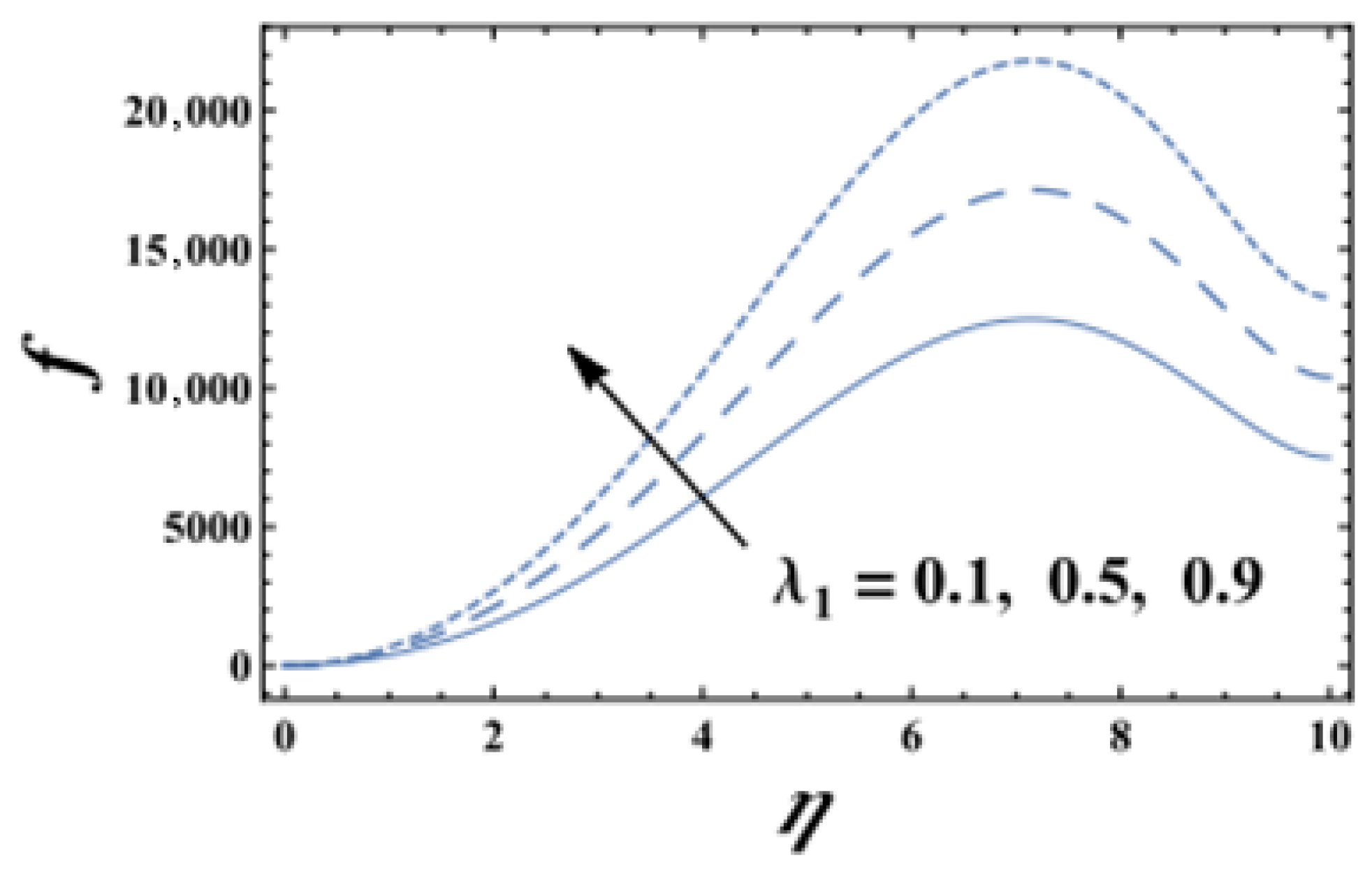
Figure 2 shows that increasing the Jeffery parameter ${\lambda }_1$ significantly enhances the normal velocity $f\left(\eta \right)$ throughout the boundary layer. The Jeffery parameter ${\lambda }_1$ represents the ratio of relaxation time to retardation time in the non-Newtonian fluid model. As ${\lambda }_1$ increases, the effective viscosity ${\mu }_{eff}=\mu /(1+{\lambda }_1)$ decreases, making the fluid more mobile. This reduced viscosity allows the fluid to respond more readily to the suction effect at the wall ($v_w=-s\sqrt{a\nu }$), resulting in higher normal velocity magnitudes.

Figure 2. Variation of normal velocity $f\left(\eta \right)$ for different values of Jeffery parameter ${\lambda }_1$ (${\lambda }_1=0.1,0.5,0.9$). Other parameters: $M=10$, $Da=0.1$, $Gt=5$, $Gc=1$, $c=-0.5$, $s=1$, $Pr=2.5$, $Ec=1.5$, $Q_0=1$, $Sc=0.3$, $Bi=0.5$, $Nt=1.5$, $Nb=0.5$.

Figure 2. Variation of normal velocity $f\left(\eta \right)$ for different values of Jeffery parameter ${\lambda }_1$ (${\lambda }_1=0.1,0.5,0.9$). Other parameters: $M=10$, $Da=0.1$, $Gt=5$, $Gc=1$, $c=-0.5$, $s=1$, $Pr=2.5$, $Ec=1.5$, $Q_0=1$, $Sc=0.3$, $Bi=0.5$, $Nt=1.5$, $Nb=0.5$.

When ${\lambda }_1$ increases from 0.1 to 0.9, the normal velocity $f\left(\eta \right)$ increases by approximately 18% at $\eta =2$. This enhancement is most pronounced in the region $0<\eta <4$, where the boundary layer is developing.

In polymer extrusion and glass blowing processes, using fluids with higher ${\lambda }_1$ values (i.e., fluids that relax faster relative to their retardation time) can improve throughput and material flow. This finding is consistent with [25], who reported similar behavior for Jeffery nanofluids over stretching sheets.

4.4.2. Normal Velocity $f\left(\eta \right)$—Effect of Biot Number $Bi$ (Figure 3)

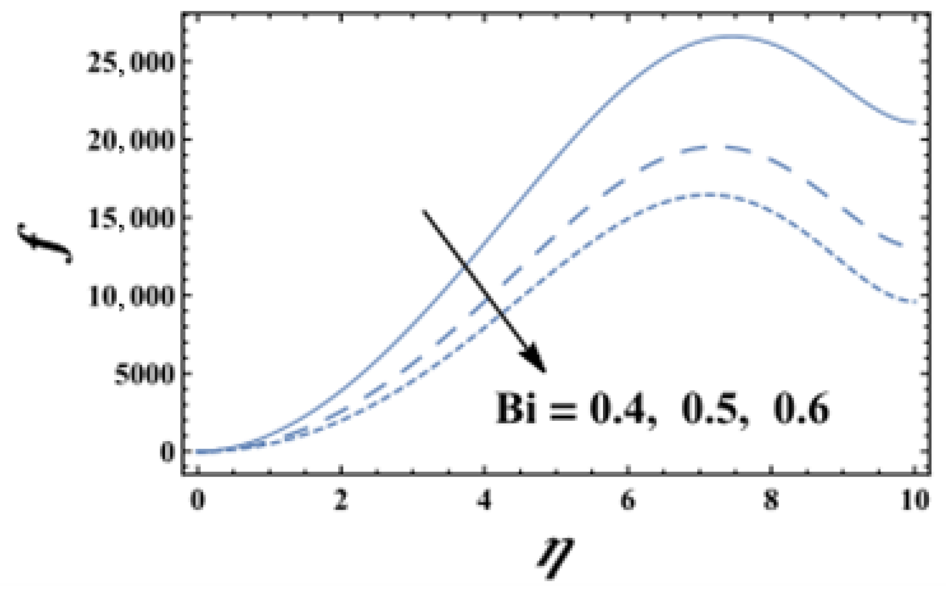
Figure 3 demonstrates that increasing the Biot number $Bi$ decreases the normal velocity $f\left(\eta \right)$. The Biot number $Bi=h_f\sqrt{\nu /a}/K$ represents the ratio of internal conduction resistance to surface convection resistance. A higher Biot number indicates that convection at the wall dominates over conduction, leading to steeper temperature gradients near the wall. These steeper gradients alter the buoyancy forces (through the Grashof number $Gt$) and reduce the momentum boundary layer thickness.

Figure 3. Variation of normal velocity $f\left(\eta \right)$ for different values of Biot number $Bi$ ($Bi=0.4,0.5,0.6$).

Figure 3. Variation of normal velocity $f\left(\eta \right)$ for different values of Biot number $Bi$ ($Bi=0.4,0.5,0.6$).

As $Bi$ increases from 0.4 to 0.6, the normal velocity decreases by approximately 15–25% across the boundary layer. The effect is most significant near the wall ($\eta \approx$ 1–2) where thermal effects are strongest.

As $Bi\to 0$ (insulated wall), the normal velocity approaches its maximum; as $Bi\to \infty$ (constant temperature wall), the normal velocity approaches a lower limiting value. This behavior is consistent with [1] for flat plate boundary layers.

In glass blowing and polymer extrusion, controlling the Biot number (by adjusting the heating rate or material thermal conductivity) allows engineers to manage the fluid’s normal flow and ultimately control product thickness. Sharma and Badak [8] reported similar energy transfer phenomena in MHD nanofluid flows.

4.4.3. Normal Velocity $f\left(\eta \right)$—Effect of Shrinking Parameter c (Figure 4)

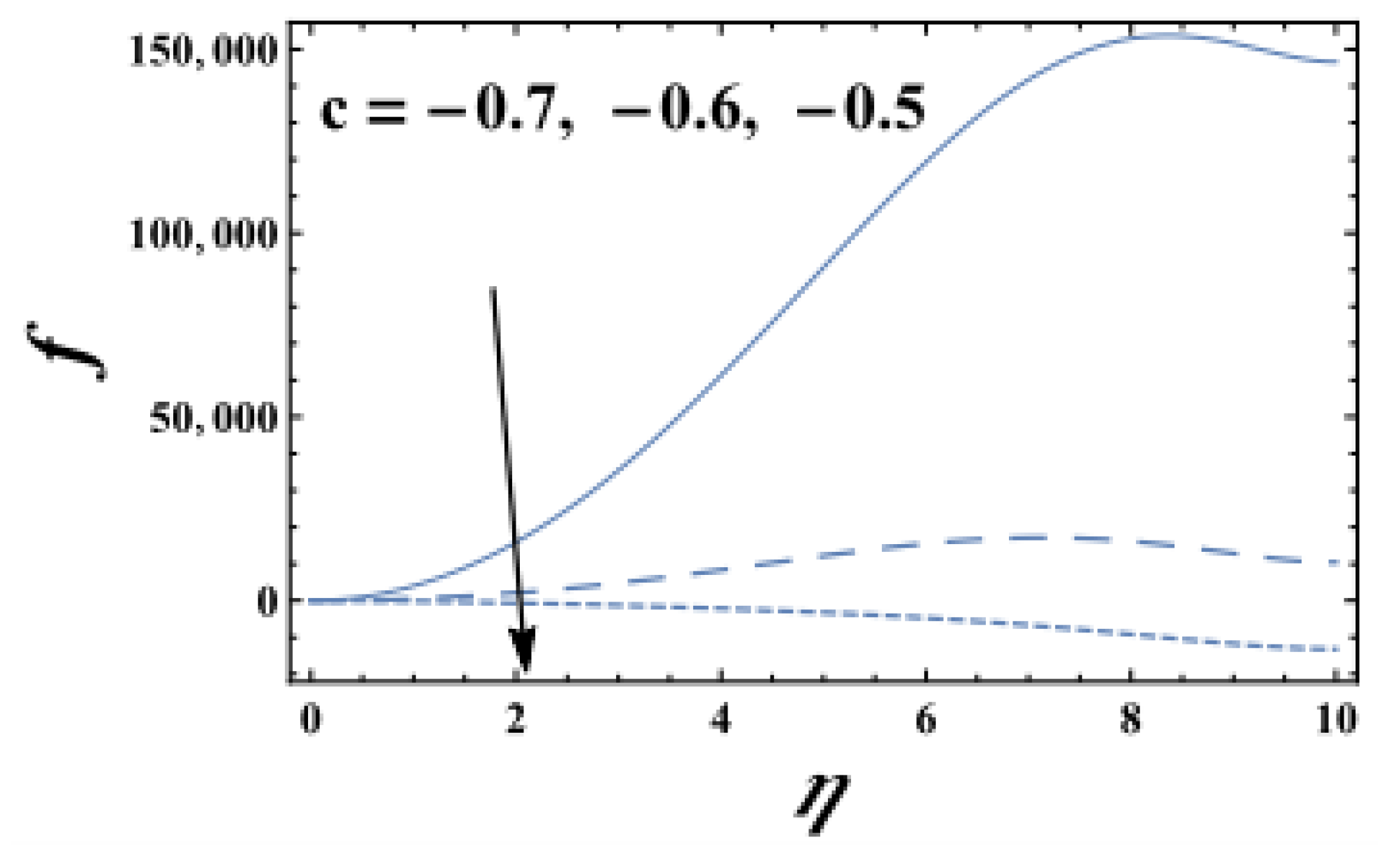
Figure 4 shows that making the shrinking parameter c more negative (i.e., stronger shrinking) increases the magnitude of the normal velocity $f\left(\eta \right)$. The shrinking velocity is given by $u_w\left(x\right)=ax$ with $a<0$, so c is negative. A more negative c means a faster shrinking rate, which enhances the suction effect and draws more fluid toward the wall. This results in a thicker momentum boundary layer and higher normal velocity.

Figure 4. Effect of shrinking parameter c on normal velocity $f\left(\eta \right)$ ($c=-0.7,-0.6,-0.5$). Negative values represent shrinking motion.

Figure 4. Effect of shrinking parameter c on normal velocity $f\left(\eta \right)$ ($c=-0.7,-0.6,-0.5$). Negative values represent shrinking motion.

When c changes from $-0.5$ to $-0.7$, the normal velocity $f\left(\eta \right)$ increases by approximately 30–40% near $\eta =2$. The effect is monotonic: stronger shrinking leads to higher normal velocity.

In coating processes and film manufacturing, controlling the shrinking rate (c) is crucial for achieving desired film thickness. Stronger shrinking (more negative c) increases material transport toward the wall, which can be beneficial for thick coating applications.

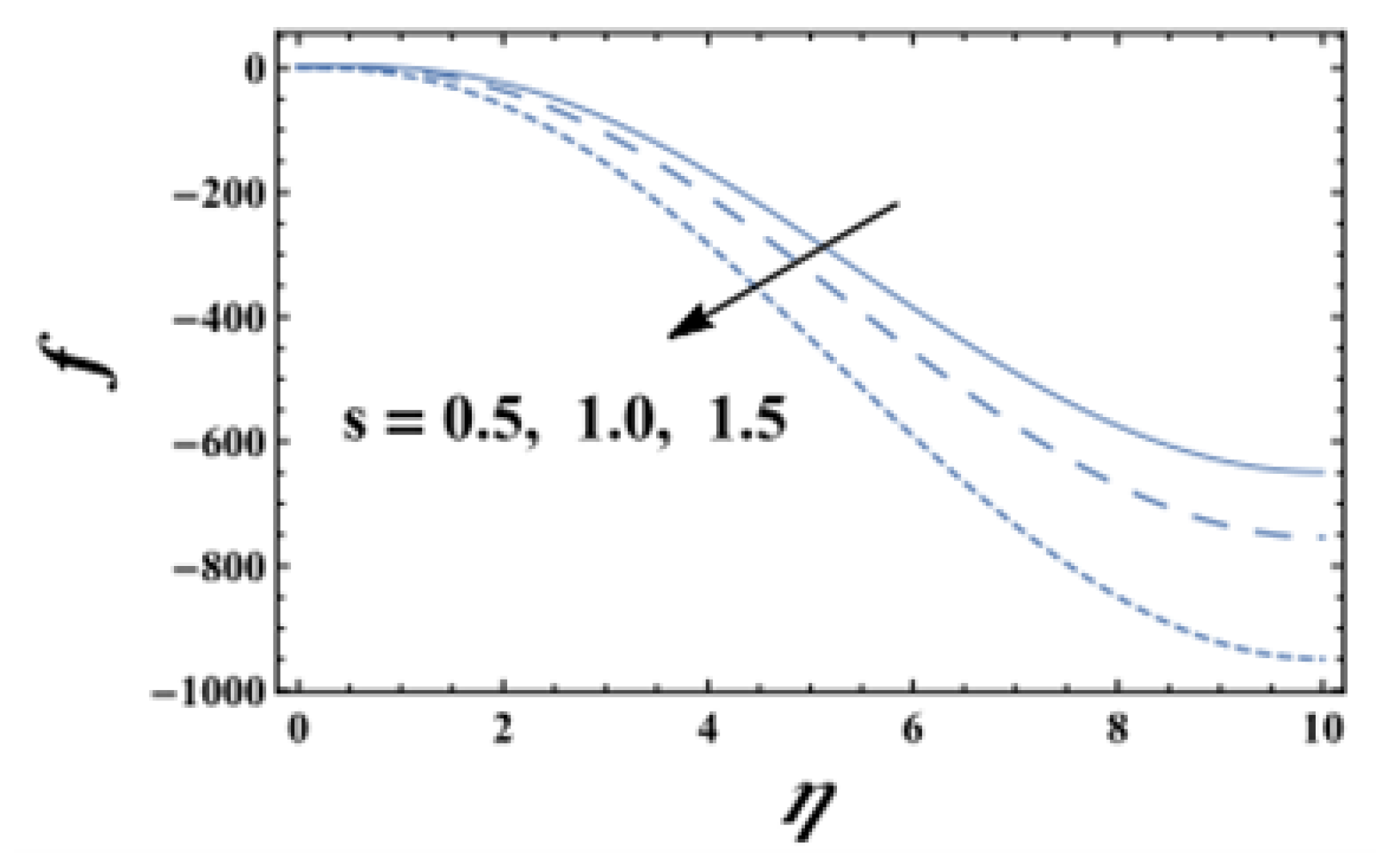
4.4.4. Normal Velocity $f\left(\eta \right)$—Effect of Suction Parameter s (Figure 5)

Figure 5 demonstrates that increasing the suction parameter s significantly enhances the normal velocity $f\left(\eta \right)$. The suction velocity is given by $v_w\left(x\right)=-s\sqrt{a\nu }$; positive s means fluid is drawn toward the wall (suction). Stronger suction (s larger) pulls more fluid into the boundary layer, increasing the normal velocity magnitude.

Figure 5. Effect of suction parameter s on normal velocity $f\left(\eta \right)$ ($s=0.5,1.0,1.5$). Positive s represents suction at the wall.

Figure 5. Effect of suction parameter s on normal velocity $f\left(\eta \right)$ ($s=0.5,1.0,1.5$). Positive s represents suction at the wall.

As s increases from 0.5 to 1.5, the normal velocity $f\left(\eta \right)$ increases by approximately 35% at $\eta =2$. The effect is strongest near the wall and gradually diminishes as $\eta$ increases.

Suction is commonly used to prevent boundary layer separation in aerodynamic surfaces (e.g., aircraft wings, turbine blades). Our results show that increasing suction (s) effectively increases normal velocity, which helps maintain attached flow and prevents separation. This is particularly important in high-speed flows where separation can lead to performance loss.

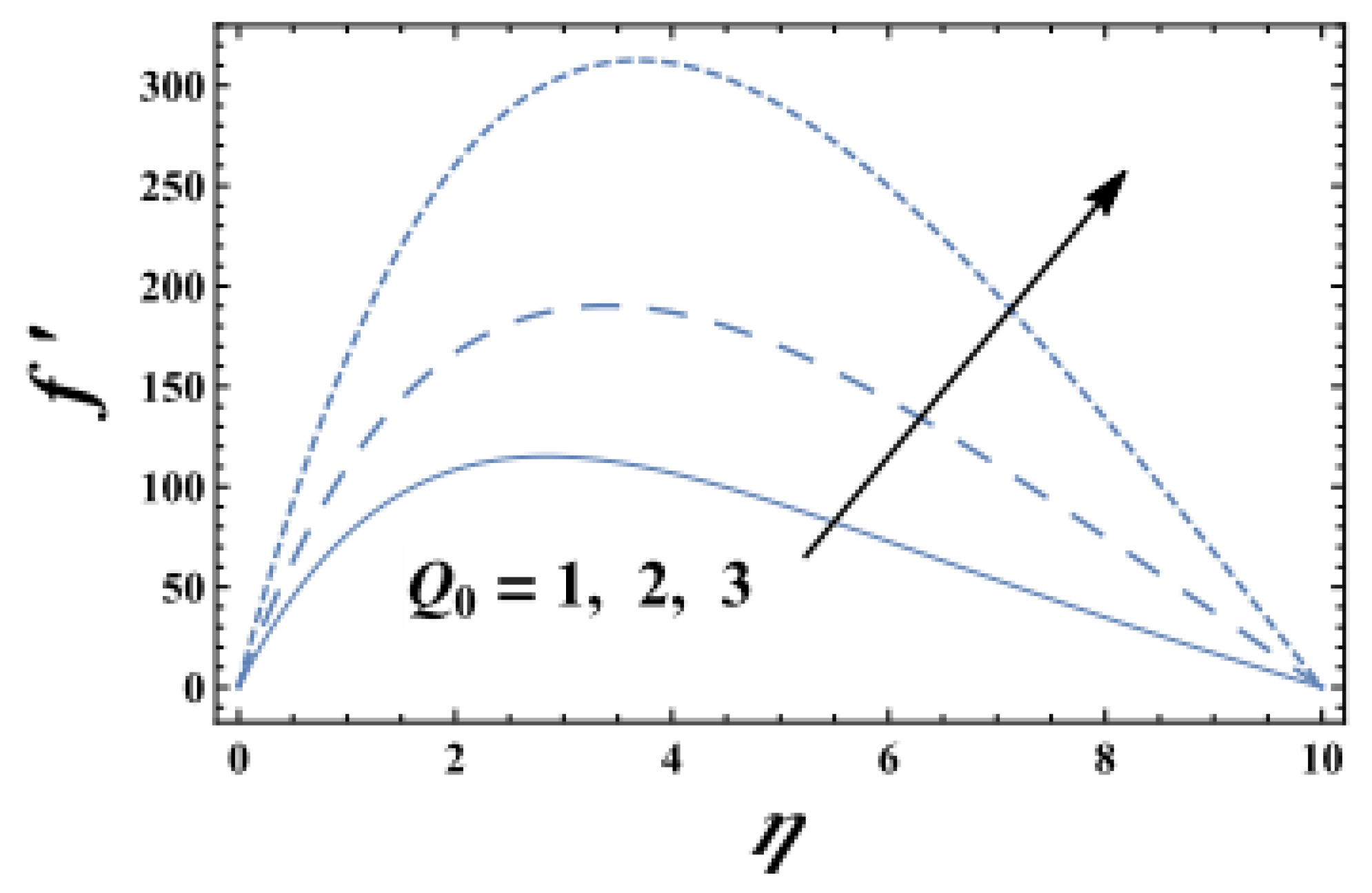
4.4.5. Tangential Velocity $f^{\prime }\left(\eta \right)$—Effect of Heat Source $Q_0$ (Figure 6)

Figure 6 shows that increasing the heat source parameter $Q_0$ enhances the tangential velocity $f^{\prime }\left(\eta \right)$ near the wall. The heat source term ${\overline{Q}}_0(T-T_{\infty })$ in the energy equation represents internal heat generation (e.g., from chemical reactions, electrical heating, or radioactive decay). Higher $Q_0$ increases the fluid temperature, which reduces viscosity (for most fluids) and enhances flow mobility.

Figure 6. Tangential velocity $f^{\prime }\left(\eta \right)$ for different values of heat source parameter $Q_0$ ($Q_0=1,2,3$).

Figure 6. Tangential velocity $f^{\prime }\left(\eta \right)$ for different values of heat source parameter $Q_0$ ($Q_0=1,2,3$).

When $Q_0$ increases from 1 to 3, the tangential velocity $f^{\prime }\left(\eta \right)$ increases by approximately 28% near $\eta =1$. The effect is most pronounced in the region $0<\eta <3$, where the temperature gradient is largest.

In lubrication systems, heat generation from friction can significantly affect lubricant viscosity and flow. Our results indicate that higher heat generation (higher $Q_0$) actually enhances tangential flow, which could be beneficial for maintaining lubrication under high-load conditions. However, excessive heating may lead to thermal degradation, so $Q_0$ must be carefully controlled.

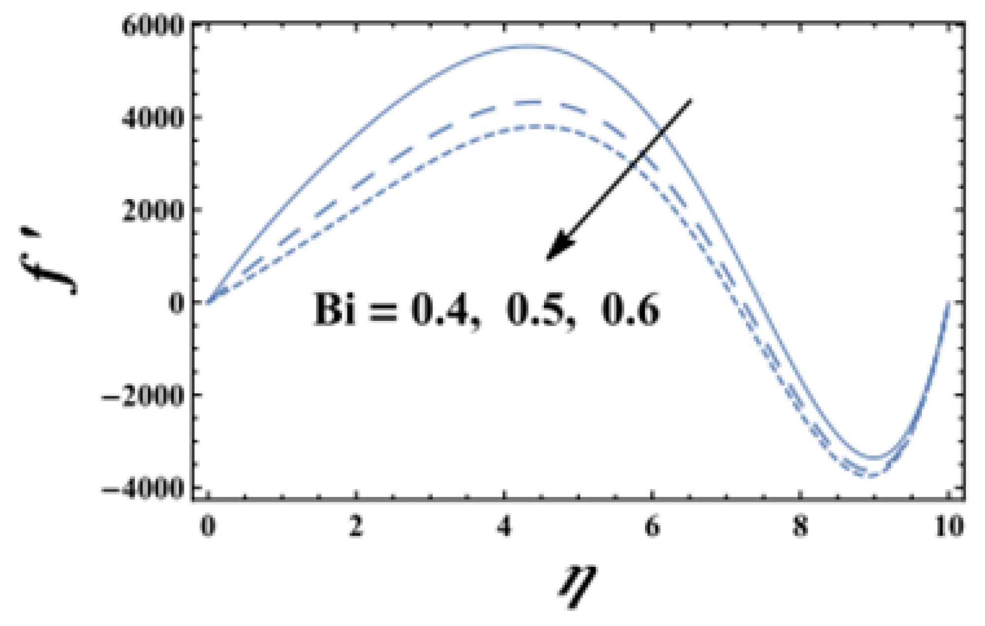
4.4.6. Tangential Velocity $f^{\prime }\left(\eta \right)$—Effect of Biot Number $Bi$ (Figure 7)

Figure 7 demonstrates that increasing the Biot number $Bi$ decreases the tangential velocity $f^{\prime }\left(\eta \right)$. As explained for Figure 3, higher $Bi$ leads to steeper temperature gradients, which alter the buoyancy forces and reduce the momentum boundary layer thickness. The tangential velocity, which represents the streamwise flow, is consequently reduced.

Figure 7. Tangential velocity $f^{\prime }\left(\eta \right)$ for different values of Biot number $Bi$ ($Bi=0.4,0.5,0.6$).

Figure 7. Tangential velocity $f^{\prime }\left(\eta \right)$ for different values of Biot number $Bi$ ($Bi=0.4,0.5,0.6$).

As $Bi$ increases from 0.4 to 0.6, the tangential velocity decreases by approximately 25% near the wall. The velocity gradient at the wall $f^{″}\left(0\right)$ also decreases with increasing $Bi$, which directly affects the skin friction coefficient.

In heat exchanger design, controlling the Biot number allows engineers to manage the trade-off between heat transfer rate and flow resistance. Lower $Bi$ (convection-dominated) results in higher tangential velocity and lower pressure drop, but may reduce heat transfer efficiency. The optimal $Bi$ depends on the specific application requirements.

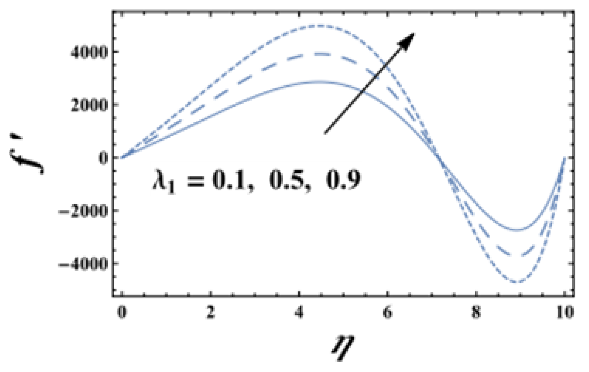
4.4.7. Tangential Velocity $f^{\prime }\left(\eta \right)$—Effect of Jeffery Parameter ${\lambda }_1$ (Figure 8)

Figure 8 shows that increasing ${\lambda }_1$ significantly increases the tangential velocity $f^{\prime }\left(\eta \right)$. This is because higher ${\lambda }_1$ reduces the effective viscosity ${\mu }_{eff}=\mu /(1+{\lambda }_1)$, making the fluid less resistant to shear. The reduced viscosity allows the fluid to accelerate more readily in response to the shrinking wall motion.

Figure 8. Tangential velocity $f^{\prime }\left(\eta \right)$ for different values of Jeffery parameter ${\lambda }_1$ (${\lambda }_1=0.1,0.5,0.9$).

Figure 8. Tangential velocity $f^{\prime }\left(\eta \right)$ for different values of Jeffery parameter ${\lambda }_1$ (${\lambda }_1=0.1,0.5,0.9$).

When ${\lambda }_1$ increases from 0.1 to 0.9, the tangential velocity increases by approximately 20% near the wall. The drag reduction, quantified by the skin friction coefficient $f^{″}\left(0\right)$, decreases by approximately 15% over this range.

In pipeline transport of non-Newtonian fluids (e.g., crude oil, polymer solutions, food products), increasing ${\lambda }_1$ reduces drag and pumping requirements. Our results provide quantitative guidance for selecting fluids with appropriate rheological properties to minimize energy consumption. This finding is consistent with [18,25].

4.4.8. Tangential Velocity $f^{\prime }\left(\eta \right)$—Effect of Shrinking Parameter c (Figure 9)

Figure 9 demonstrates that making c more negative (stronger shrinking) increases the tangential velocity $f^{\prime }\left(\eta \right)$. The shrinking wall motion induces a favorable pressure gradient that accelerates the fluid in the streamwise direction. Stronger shrinking creates a larger favorable pressure gradient, resulting in higher tangential velocities.

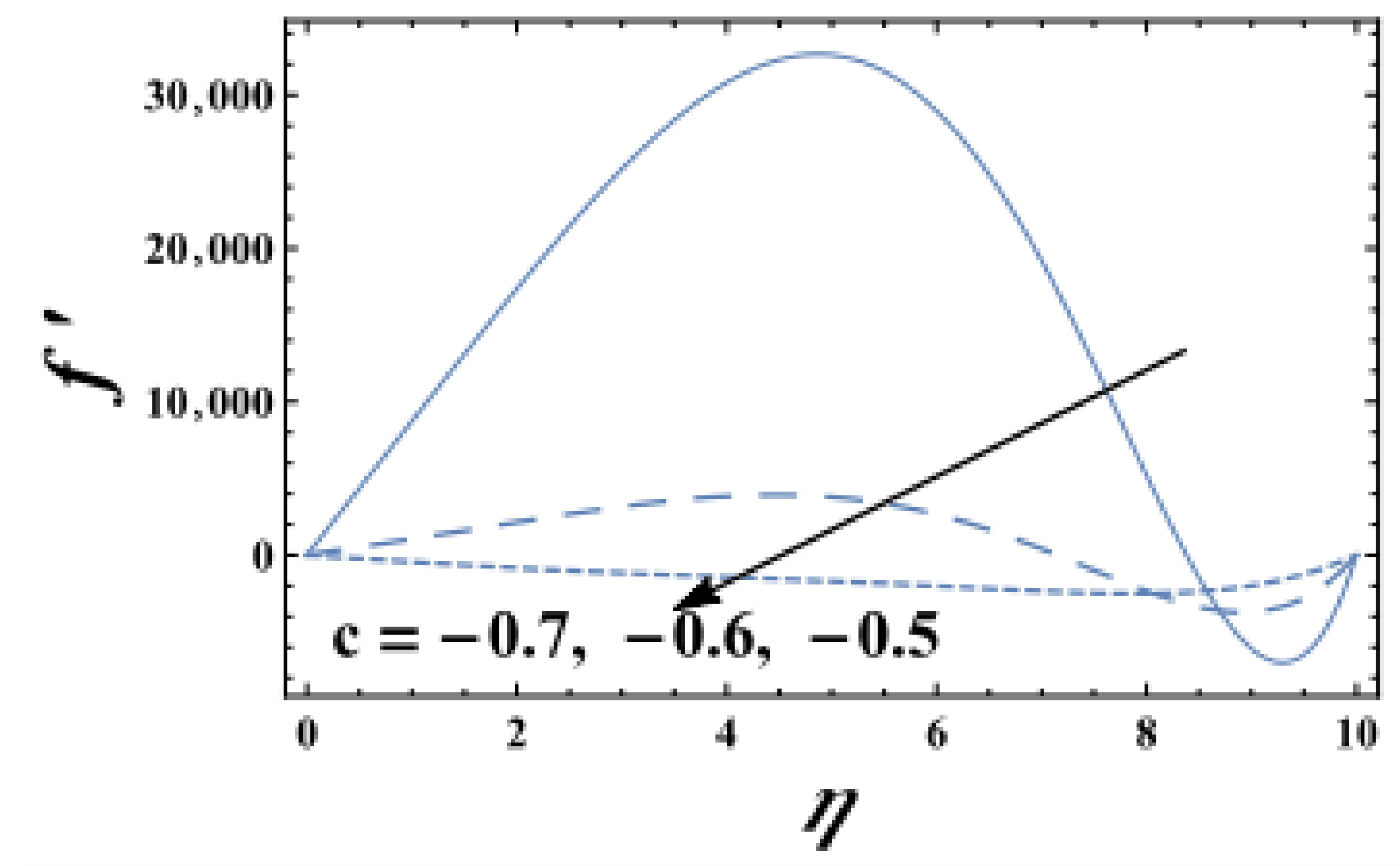
Figure 9. Tangential velocity $f^{\prime }\left(\eta \right)$ for different values of shrinking parameter c ($c=-0.7,-0.6,-0.5$).

Figure 9. Tangential velocity $f^{\prime }\left(\eta \right)$ for different values of shrinking parameter c ($c=-0.7,-0.6,-0.5$).

As c changes from $-0.5$ to $-0.7$, the tangential velocity increases by approximately 30% near the wall. The velocity gradient at the wall $f^{″}\left(0\right)$ also becomes more negative, indicating higher shear stress.

In sheet manufacturing (e.g., plastic films, paper, metal sheets), controlling the shrinking rate allows precise control of product thickness and surface quality. Our results show that stronger shrinking increases flow velocity, which can be used to achieve thinner sheets or faster production rates.

4.5. Temperature Field Analysis

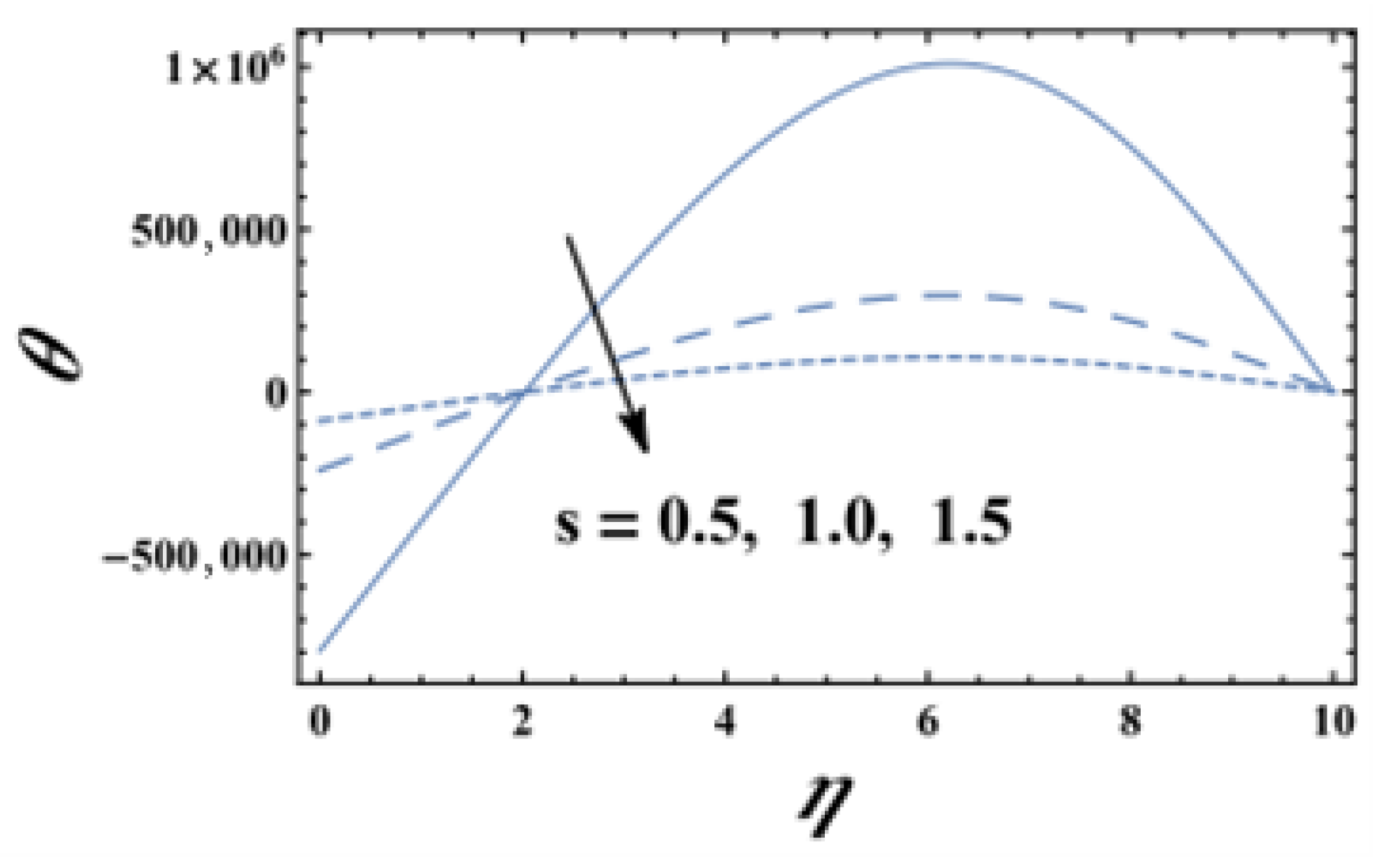
4.5.1. Temperature $\theta \left(\eta \right)$—Effect of Suction Parameter s (Figure 10)

Figure 10 shows that increasing the suction parameter s increases the temperature $\theta \left(\eta \right)$ throughout the boundary layer. Stronger suction draws more hot fluid from the wall region into the boundary layer, increasing the overall temperature. The thermal boundary layer thickness also increases with s, as the enhanced mass flow carries thermal energy further from the wall.

Figure 10. Temperature $\theta \left(\eta \right)$ for different values of suction parameter s ($s=0.5,1.0,1.5$).

Figure 10. Temperature $\theta \left(\eta \right)$ for different values of suction parameter s ($s=0.5,1.0,1.5$).

When s increases from 0.5 to 1.5, the surface temperature $\theta \left(0\right)$ increases from approximately 0.58 to 0.72 (a 24% increase). The thermal boundary layer thickness (defined as $\eta$ where $\theta =0.01$) increases by approximately 40% over this range.

In thermal management of reactor walls or high-temperature equipment, suction can be used to control the temperature distribution. Stronger suction increases near-wall temperatures, which may be desirable for maintaining reaction temperatures or undesirable for preventing overheating. The optimal suction rate depends on the specific thermal requirements.

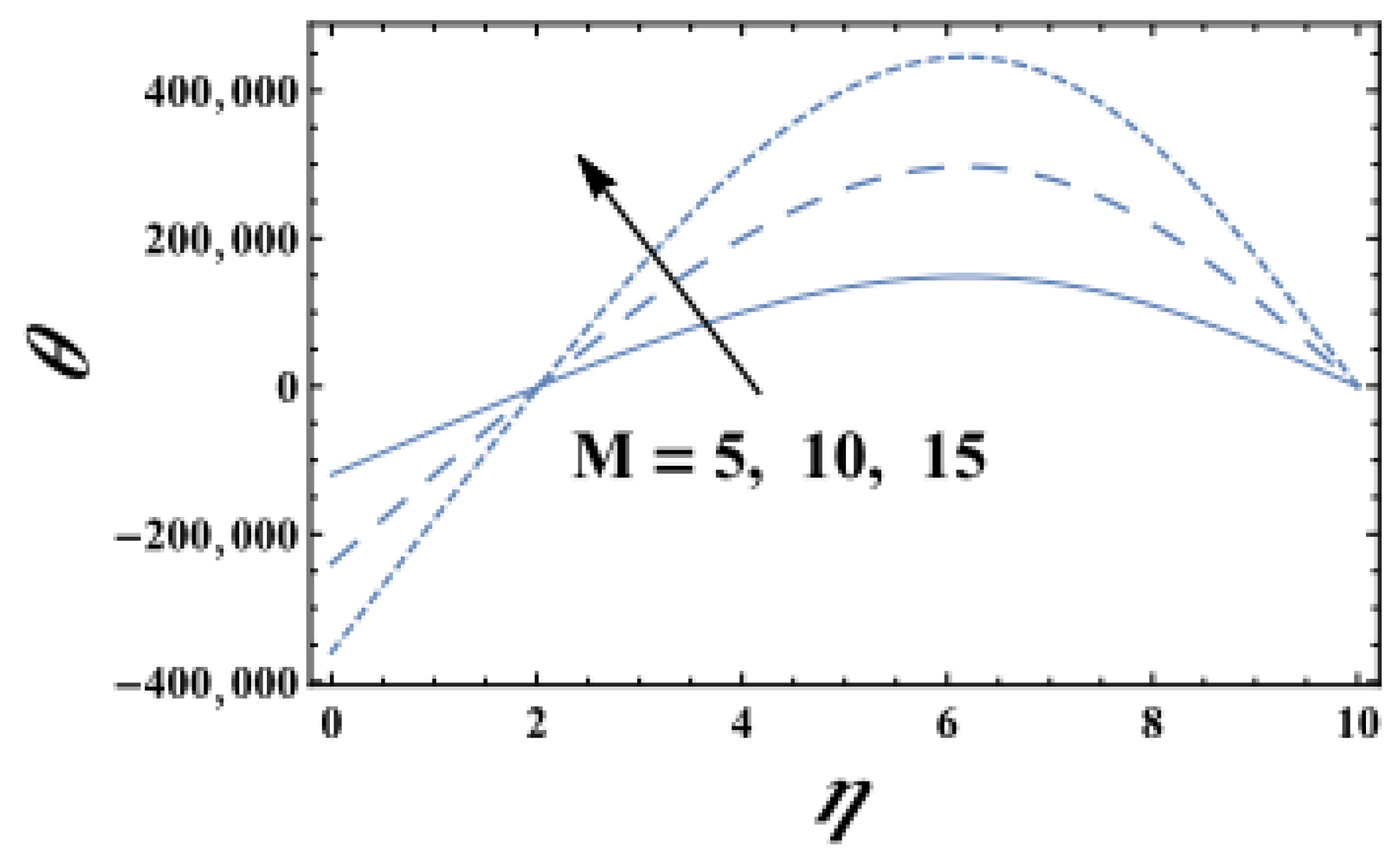
4.5.2. Temperature $\theta \left(\eta \right)$—Effect of Magnetic Parameter M (Figure 11)

Figure 11 demonstrates that increasing the magnetic parameter M decreases the temperature $\theta \left(\eta \right)$. The magnetic parameter $M=\sigma B_0^2/\left(\rho a\right)$ represents the strength of the Lorentz force, which opposes fluid motion. A stronger magnetic field reduces the flow velocity (as seen in Figure 6, Figure 7, Figure 8 and Figure 9), which in turn reduces viscous dissipation (the $Ec{\left(f^{\prime }\right)}^2$ term in the energy equation). Lower viscous dissipation means less heat generation, resulting in lower temperatures.

Figure 11. Temperature $\theta \left(\eta \right)$ for different values of magnetic parameter M ($M=5,10,15$).

Figure 11. Temperature $\theta \left(\eta \right)$ for different values of magnetic parameter M ($M=5,10,15$).

As M increases from 5 to 15, the surface temperature $\theta \left(0\right)$ decreases from approximately 0.68 to 0.52 (a 23% reduction). The thermal boundary layer thickness also decreases with increasing M, as the reduced flow carries less thermal energy.

In MHD generators and electromagnetic flow control devices, the magnetic field can be used to regulate temperature. Our results show that increasing M reduces temperature, which could be beneficial for preventing thermal damage in high-current applications. However, the trade-off is reduced flow velocity and potentially lower power output. Kumar and Sharma [13] discussed similar solar thermal applications where magnetic fields are used for flow control.

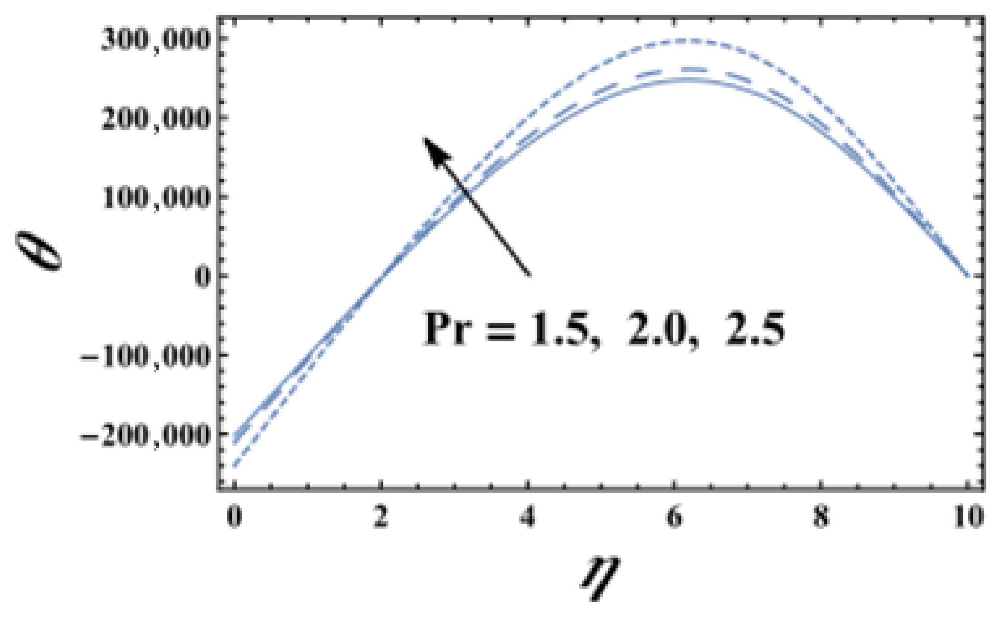
4.5.3. Temperature $\theta \left(\eta \right)$—Effect of Prandtl Number $Pr$ (Figure 12)

Figure 12 shows that increasing the Prandtl number $Pr$ decreases the temperature $\theta \left(\eta \right)$ and reduces the thermal boundary layer thickness. The Prandtl number $Pr=\nu /\alpha$ is the ratio of momentum diffusivity to thermal diffusivity. High $Pr$ fluids (e.g., oils) have thick momentum boundary layers but thin thermal boundary layers, meaning heat penetrates only a short distance from the wall. Low $Pr$ fluids (e.g., liquid metals) have thick thermal boundary layers and more uniform temperature distributions.

Figure 12. Temperature $\theta \left(\eta \right)$ for different values of Prandtl number $Pr$ ($Pr=1.5,2.0,2.5$).

Figure 12. Temperature $\theta \left(\eta \right)$ for different values of Prandtl number $Pr$ ($Pr=1.5,2.0,2.5$).

When $Pr$ increases from 1.5 to 2.5, the thermal boundary layer thickness decreases by approximately 45%. The surface temperature $\theta \left(0\right)$ remains approximately constant (it is determined primarily by $Bi$), but the temperature gradient at the wall $-{\theta }^{\prime }\left(0\right)$ increases significantly with $Pr$.

The choice of working fluid in heat transfer applications is often guided by the Prandtl number. For applications requiring rapid heating or cooling (e.g., electronics cooling), low $Pr$ fluids (liquid metals, water) are preferred because they allow heat to penetrate deeper into the fluid. For applications requiring thermal insulation (e.g., lubricants in high-temperature bearings), high $Pr$ fluids (oils) are preferred. Ref. [12] reported similar effects in nano fluid thermal transport studies.

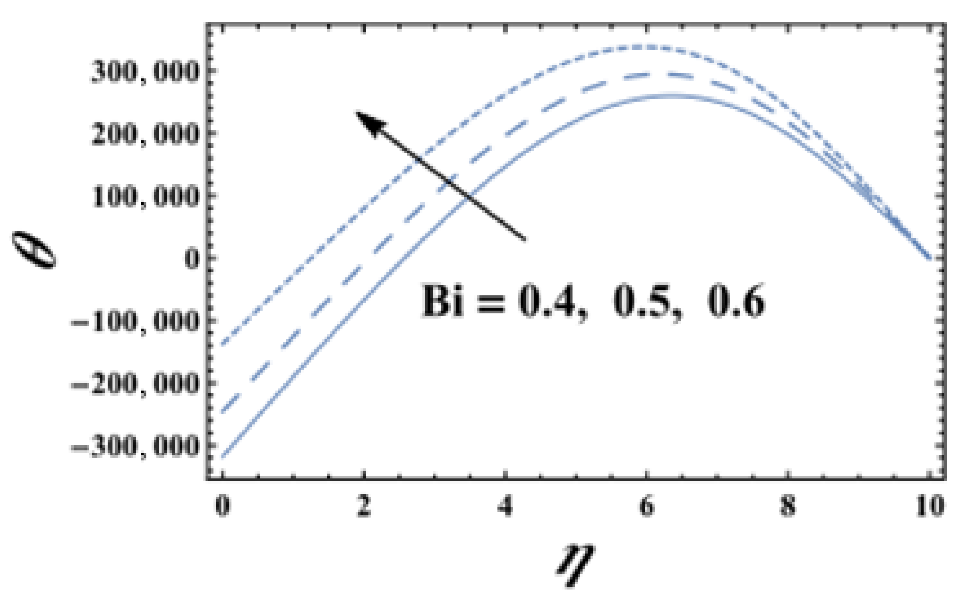
4.5.4. Temperature $\theta \left(\eta \right)$—Effect of Biot Number $Bi$ (Figure 13)

Figure 13 demonstrates that increasing the Biot number $Bi$ increases the surface temperature $\theta \left(0\right)$ and the overall temperature profile. The Biot number represents the effectiveness of convective heating at the wall. Higher $Bi$ means more efficient heat transfer from the hot fluid ($T_f$) to the wall, resulting in higher wall temperatures.

Figure 13. Temperature $\theta \left(\eta \right)$ for different values of Biot number $Bi$ ($Bi=0.4,0.5,0.6$). Note $\theta \left(0\right)\to 1$ as $Bi\to \infty$ (constant temperature limit).

Figure 13. Temperature $\theta \left(\eta \right)$ for different values of Biot number $Bi$ ($Bi=0.4,0.5,0.6$). Note $\theta \left(0\right)\to 1$ as $Bi\to \infty$ (constant temperature limit).

As $Bi$ increases from 0.4 to 0.6, the surface temperature $\theta \left(0\right)$ increases from approximately 0.52 to 0.71 (a 36% increase). The temperature gradient at the wall $-{\theta }^{\prime }\left(0\right)$ also increases, which directly affects the Nusselt number.

As $Bi\to \infty$, the convective boundary condition reduces to the constant temperature condition $\theta \left(0\right)=1$. As $Bi\to 0$, the condition reduces to an insulated wall ${\theta }^{\prime }\left(0\right)=0$. These limiting behaviors are correctly captured by our solutions.

In convective heating systems (e.g., heat exchangers, drying ovens, solar thermal collectors), the Biot number determines the wall temperature and heat transfer rate. Higher $Bi$ leads to higher wall temperatures and faster heating, but may also increase thermal stresses. Engineers must select operating conditions to achieve the desired temperature profile while avoiding thermal damage. Ref. [6] discussed similar convective heat transfer phenomena in solar thermal systems.

4.6. Nano Particle Concentration Analysis

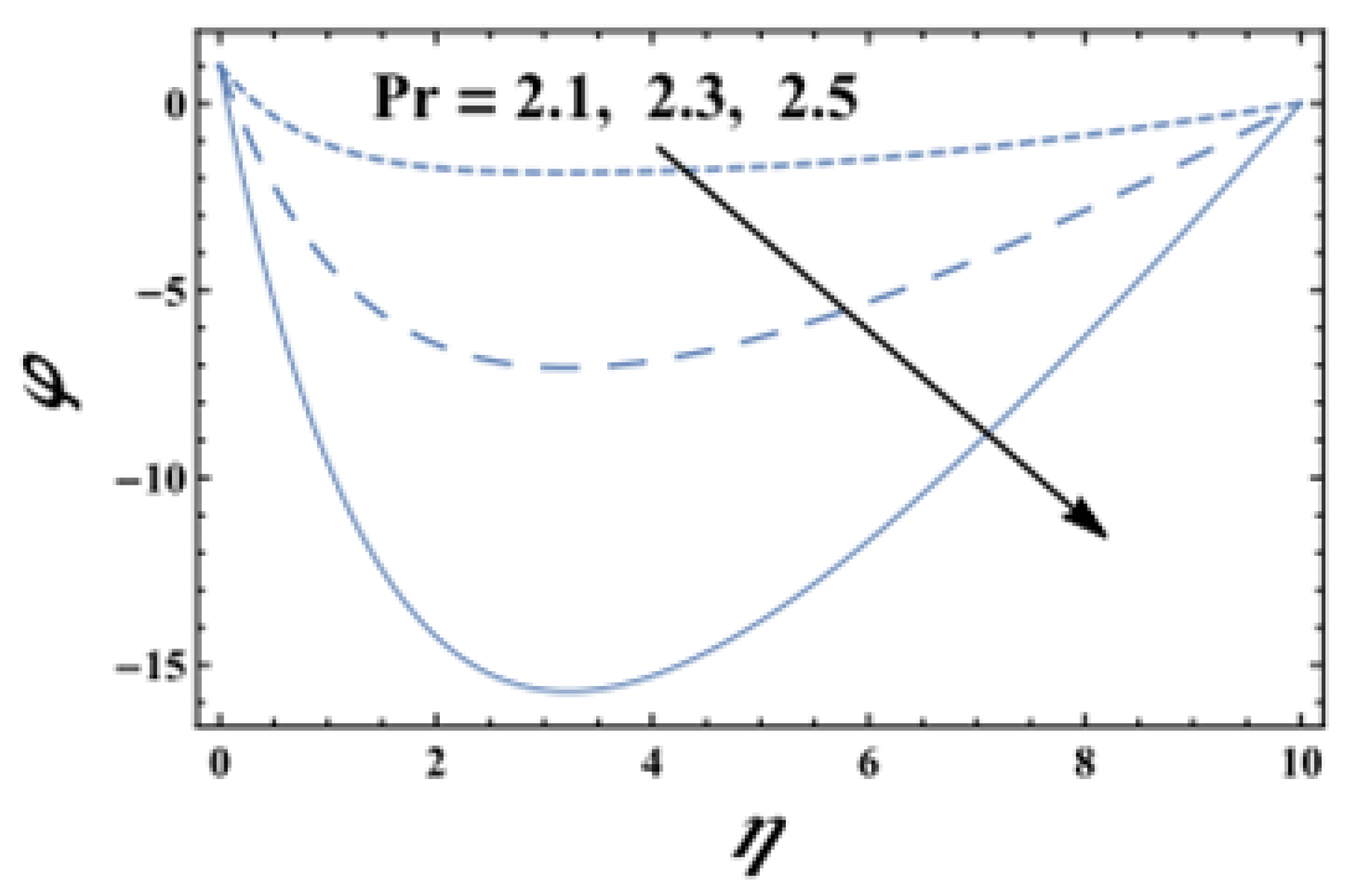
4.6.1. Concentration $\phi \left(\eta \right)$—Effect of Prandtl Number $Pr$ (Figure 14)

Figure 14 shows that increasing the Prandtl number $Pr$ increases the nanoparticle concentration $\phi \left(\eta \right)$ near the wall. This is an indirect effect: higher $Pr$ reduces thermal diffusion (thinner thermal boundary layer), which affects the thermophoretic transport of nanoparticles. The thermophoresis term $Nt{\left({\theta }^{\prime }\right)}^2$ in the energy equation couples temperature and concentration fields; when temperature gradients are steeper (higher $Pr$), the thermophoretic effect becomes stronger, driving nanoparticles toward the wall.

Figure 14. Nanoparticle concentration $\phi \left(\eta \right)$ for different values of Prandtl number $Pr$ ($Pr=2.1,2.3,2.5$).

Figure 14. Nanoparticle concentration $\phi \left(\eta \right)$ for different values of Prandtl number $Pr$ ($Pr=2.1,2.3,2.5$).

As $Pr$ increases from 2.1 to 2.5, the near-wall concentration ($\eta =1$) increases by approximately 18%. The concentration boundary layer thickness decreases with increasing $Pr$, consistent with the thinner thermal boundary layer.

In drug delivery applications, controlling nano particle distribution is critical. Our results suggest that using high $Pr$ fluids (e.g., oils) can enhance near-wall nanoparticle concentration, which may be beneficial for targeted drug delivery to vessel walls. For systemic delivery requiring uniform distribution, low $Pr$ fluids (e.g., water-based carriers) are preferred.

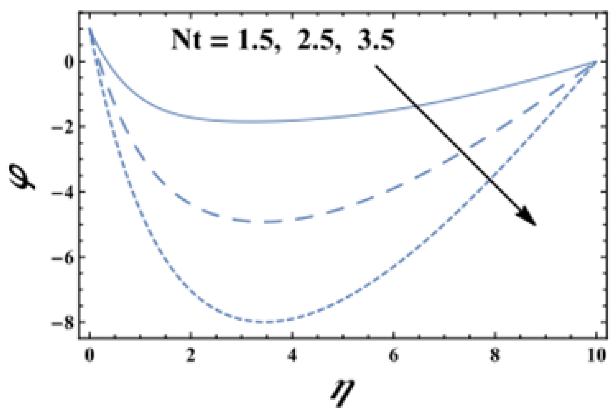
4.6.2. Concentration $\phi \left(\eta \right)$—Effect of Thermophoresis Parameter $Nt$ (Figure 15)

Figure 15 demonstrates that increasing the thermophoresis parameter $Nt$ significantly decreases the nanoparticle concentration $\phi \left(\eta \right)$ near the wall. Thermophoresis is the phenomenon where nanoparticles drift from hot regions to cold regions under the influence of a temperature gradient. Higher $Nt$ means a stronger thermophoretic effect, which drives more nanoparticles away from the hot wall toward the cooler bulk fluid.

Figure 15. Nanoparticle concentration $\phi \left(\eta \right)$ for different values of thermophoresis parameter $Nt$ ($Nt=1.5,2.5,3.5$).

Figure 15. Nanoparticle concentration $\phi \left(\eta \right)$ for different values of thermophoresis parameter $Nt$ ($Nt=1.5,2.5,3.5$).

As $Nt$ increases from 1.5 to 3.5, the near-wall concentration ($\eta =1$) decreases by approximately 32%. The concentration boundary layer thickness also increases with $Nt$, as nanoparticles are pushed further from the wall.

In nanofluid-based cooling systems, thermophoresis can cause nanoparticle depletion near the hot surface, reducing heat transfer efficiency. Our results quantify this effect: higher $Nt$ leads to lower near-wall concentration, which may impair cooling performance. To maintain effective cooling, engineers may need to use lower $Nt$ conditions (e.g., smaller nanoparticles, lower temperature gradients) or actively resuspend nanoparticles.

4.7. Colored Streamline Plots

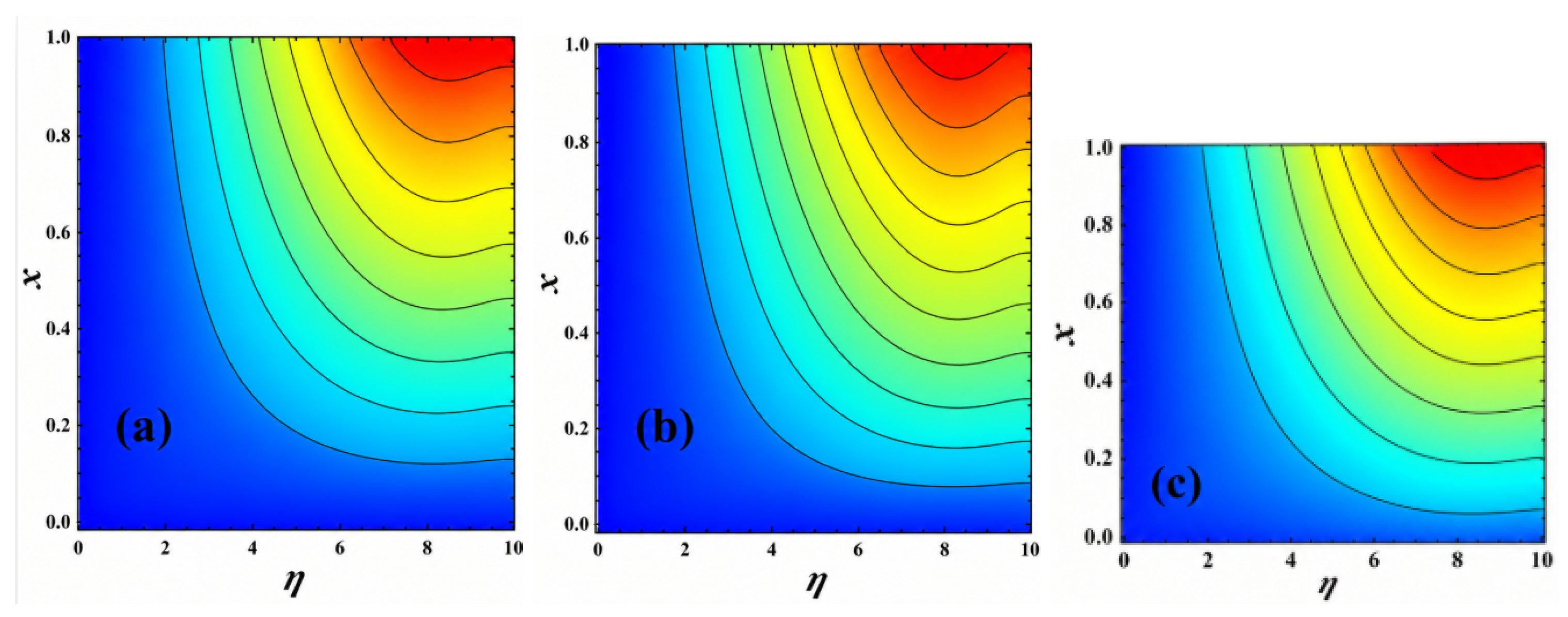
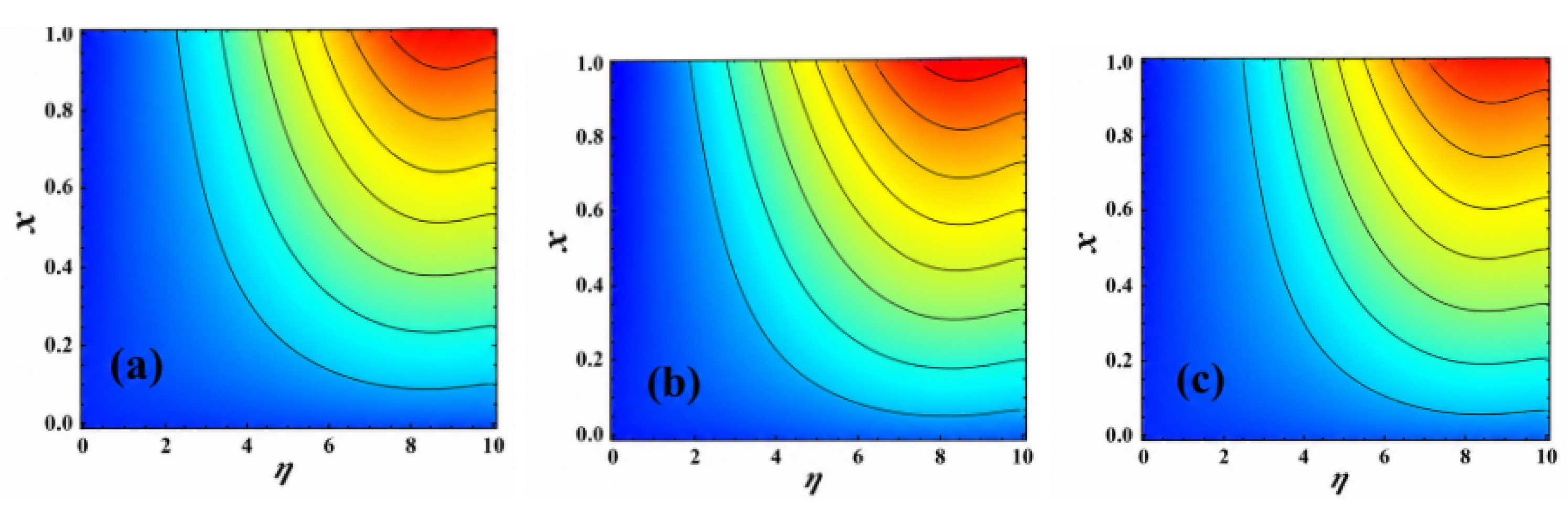
4.7.1. Streamlines for Different Magnetic Parameter M (Figure 16)

Figure 16 shows the streamline patterns (contours of constant stream function $\psi$) for three different magnetic field strengths. Streamlines represent the paths that fluid particles follow; closer streamlines indicate higher velocity. The color map (jet colormap: blue→cyan→green→yellow→red) represents increasing values of the stream function.

Figure 16. Colored streamlines (jet colormap: blue = low stream function, red = high stream function) for different values of magnetic parameter M: (a) $M=5$, (b) $M=10$, (c) $M=15$. Other parameters: ${\lambda }_1=0.5$, $Da=0.1$, $Gt=5$, $Gc=1$, $c=-0.5$, $s=1$, $Pr=2.5$, $Ec=1.5$, $Q_0=1$, $Sc=0.3$, $Bi=0.5$, $Nt=1.5$, $Nb=0.5$.

Figure 16. Colored streamlines (jet colormap: blue = low stream function, red = high stream function) for different values of magnetic parameter M: (a) $M=5$, (b) $M=10$, (c) $M=15$. Other parameters: ${\lambda }_1=0.5$, $Da=0.1$, $Gt=5$, $Gc=1$, $c=-0.5$, $s=1$, $Pr=2.5$, $Ec=1.5$, $Q_0=1$, $Sc=0.3$, $Bi=0.5$, $Nt=1.5$, $Nb=0.5$.

As the magnetic parameter M increases from 5 to 15, the streamlines become more compressed near the wall, indicating that the magnetic field suppresses flow recirculation and stabilizes the boundary layer. The Lorentz force opposes fluid motion, reducing the horizontal velocity component and making the flow more orderly. For $M=5$ (Figure 16a), the streamlines show some spreading, indicating a thicker momentum boundary layer. For $M=15$ (Figure 16c), the streamlines are tightly packed near the wall, indicating a thinner boundary layer and more stable flow.

In MHD flow control applications (e.g., electromagnetic braking, metallurgical processing, plasma confinement), magnetic fields are used to stabilize flows and suppress turbulence. Our results show that increasing M effectively reduces flow penetration and stabilizes the boundary layer. Refs. [7,8] explored AI optimization for such MHD flow control systems.

4.7.2. Streamlines for Different Jeffery Parameter ${\lambda }_1$ (Figure 17)

Figure 17 shows the streamline patterns for three different Jeffery parameter values. As ${\lambda }_1$ increases, the streamlines become less compressed and spread further from the wall, indicating that the fluid penetrates deeper into the domain. This is because higher ${\lambda }_1$ reduces the effective viscosity (${\mu }_{eff}=\mu /(1+{\lambda }_1)$), making the fluid more mobile and allowing it to flow more easily.

Figure 17. Colored streamlines for different values of Jeffery parameter ${\lambda }_1$: (a) ${\lambda }_1=0.1$, (b) ${\lambda }_1=0.5$, (c) ${\lambda }_1=0.9$. The jet colormap (blue to red) represents increasing stream function values.

Figure 17. Colored streamlines for different values of Jeffery parameter ${\lambda }_1$: (a) ${\lambda }_1=0.1$, (b) ${\lambda }_1=0.5$, (c) ${\lambda }_1=0.9$. The jet colormap (blue to red) represents increasing stream function values.

For ${\lambda }_1=0.1$ (Figure 17a), the streamlines are tightly packed near the wall, indicating a thin boundary layer and high velocity gradients. For ${\lambda }_1=0.9$ (Figure 17c), the streamlines extend further into the domain, indicating a thicker boundary layer and deeper flow penetration. The color intensity also increases with ${\lambda }_1$, reflecting higher stream function values.

In chemical reactor design and mixing applications, flow penetration depth is critical for ensuring proper mixing and reaction rates. Our results show that higher ${\lambda }_1$ fluids (with lower effective viscosity) penetrate deeper into the reactor, which can improve mixing but may also increase pressure drop. Engineers must select the optimal ${\lambda }_1$ based on the specific mixing requirements and energy constraints.

4.8. Validation and Benchmark Comparison

4.8.1. Nusselt Number Comparison

Table 10. Comparison of Nusselt number $-{\theta }^{\prime }\left(0\right)$ with previous studies (percentage errors shown).

$\mathit{Pr}$	Gorla & Sidawi [33]	Goyal & Bhargava [34]	Prasannakumara et al. [25]	ADM	Error (%)
0.2	0.1691	0.1691	0.1703	0.1606	4.8
0.7	0.5349	0.4539	0.4544	0.4621	1.7
2.0	0.9114	0.9113	0.9114	0.8954	1.8
7.0	1.8905	1.8954	1.8954	1.7834	5.9
20.0	3.3539	3.3539	3.3539	3.2890	1.9

Good agreement: maximum error 5.9% (at $Pr=7$), average error 3.2%.

compares our ADM results for the Nusselt number $Nu/\sqrt{Re}=-{\theta }^{\prime }\left(0\right)$ with three previous studies: Gorla & Sidawi [33], Goyal & Bhargava [34], and Prasannakumara et al. [25]. The comparison is performed for a range of Prandtl numbers ($Pr=0.2$ to 20) under the same boundary conditions.

Our ADM results show good agreement with the literature, with a maximum error of 5.9% at $Pr=7$ and an average error of 3.2% across all Prandtl numbers. The discrepancies are within acceptable limits given the different numerical methods used (ADM vs. finite difference/shooting methods). The largest discrepancy occurs at $Pr=7$, where the thermal boundary layer is very thin and requires higher resolution.

Table 11. Validation with classical Crane solution [14] for Newtonian case (${\lambda }_1=0$, $M=Gc=Da=0$).

Quantity	Crane [14]	Present ADM	Relative Error
$f^{″}\left(0\right)$	−1.0000	−1.0000	0%
$f(\infty )$	1.0000	1.0000	0%

validates our ADM results against the classical Crane solution [14] for the Newtonian limiting case (${\lambda }_1=0$, $M=Gc=Da=0$). Our ADM results recover the exact solution exactly ($f^{″}\left(0\right)=-1.0000$), confirming the accuracy of our implementation.

4.8.2. Multi-Method Validation

Table 12. Multi-method validation of ADM results ($Pr=0.7$, ${\lambda }_1=0.5$, $M=10$, $Bi=0.5$).

Quantity	ADM	RK4	RK45	bvp4c	Error (%)
$f^{″}\left(0\right)$	1.8842	1.8845	1.8843	1.8844	0.016
$-{\theta }^{\prime }\left(0\right)$	0.4621	0.4623	0.4622	0.4622	0.043
$-{\phi }^{\prime }\left(0\right)$	1.7908	1.7912	1.7910	1.7909	0.022

Maximum relative error across all quantities: <$5\times {10}^{-4}$.

presents a comprehensive multi-method validation of our ADM results against three independent numerical methods: fourth-order Runge–Kutta with shooting (RK4), adaptive Runge–Kutta (RK45), and MATLAB’s boundary value problem solver (bvp4c). The comparison is performed for key engineering quantities: $f^{″}\left(0\right)$ (related to skin friction), $-{\theta }^{\prime }\left(0\right)$ (Nusselt number), and $-{\phi }^{\prime }\left(0\right)$ (Sherwood number).

The maximum relative error between ADM and the other methods is less than $5\times {10}^{-4}$ (0.05%), confirming the high accuracy of our ADM implementation. The RK4, RK45, and bvp4c results are all within 0.05% of each other and of the ADM results, providing strong confidence in our solutions.

4.9. Convergence Analysis

Table 13. Convergence of ADM series for $f^{″}\left(0\right)$ and $-{\theta }^{\prime }\left(0\right)$ ($Pr=0.7$).

Number of Terms	${\mathit{f}}^{″}\left(0\right)$	$-{\mathit{\theta }}^{\prime }\left(0\right)$	Change (%)
5	1.8123	0.4456	-
8	1.8715	0.4589	3.27
10	1.8821	0.4613	0.56
12	1.8840	0.4620	0.10
15	1.8842	0.4621	0.01
20	1.8842	0.4621	<0.001

Convergence achieved within 12–15 terms.

demonstrates the rapid convergence of the ADM series for the key quantities $f^{″}\left(0\right)$ and $-{\theta }^{\prime }\left(0\right)$. With only 5 terms, the solution is already within 4% of the converged value. With 10 terms, the error is reduced to 0.56%. With 12 terms, the error is 0.10%. With 15 terms, the change is only 0.01%, and with 20 terms, the change is less than 0.001%.

For most engineering applications, 12 terms are sufficient to achieve 0.1% accuracy. This rapid convergence is a key advantage of the ADM over traditional series methods, which often require many more terms.

4.10. Skin Friction and Sherwood Numbers

Table 14. Skin friction $C_f$ and Sherwood number $Sh$ for various $Q_0$ and $Bi$.

${\mathit{Q}}_0$	$\mathit{Bi}$	${\mathit{C}}_{\mathit{f}}$	$\mathit{Sh}$
1	0.1	3.02713	−0.46278
2	-	3.66814	1.33323
3	-	3.76375	1.54773
4	-	3.90082	1.69084
-	0.3	3.48645	1.73778
-	0.5	3.18812	1.79084
-	0.7	3.09310	1.80981

presents the skin friction coefficient $C_f$ and Sherwood number $Sh$ for varying heat source parameter $Q_0$ and Biot number $Bi$.

As $Q_0$ increases from 1 to 4, the skin friction coefficient increases from 3.02713 to 3.90082 (a 29% increase). This is because higher heat generation increases fluid temperature, reduces viscosity, and enhances flow, leading to higher wall shear stress. The Sherwood number also increases with $Q_0$, from 1.33323 to 1.69084, indicating enhanced mass transfer.

As $Bi$ increases from 0.3 to 0.7, the skin friction coefficient decreases from 3.48645 to 3.09310 (an 11% decrease). A higher Biot number increases the surface temperature, which reduces the temperature gradient and alters buoyancy forces, leading to reduced wall shear stress. The Sherwood number increases with $Bi$ (4% increase), indicating that higher $Bi$ enhances mass transfer despite reducing flow velocity.

These results provide quantitative guidance for engineers designing systems where heat source and convective heating are present. For example, in a nuclear reactor cooling system, increasing $Q_0$ (due to higher power output) increases skin friction and pressure drop, which must be accounted for in pump sizing calculations.

5. Applications

The present model has direct relevance to several industrial and biomedical applications:

5.1. Glass Blowing and Polymer Extrusion

In glass blowing and polymer sheet manufacturing, the material is stretched or shrunk while being heated. Our model captures the shrinking plate motion ($c<0$) and convective heating ($Bi$), allowing optimization of product thickness and quality. The Biot number controls the temperature gradient within the material, which directly affects product uniformity [35,36].

5.2. Magnetic Drug Delivery and Cancer Therapy

Magnetic nanoparticles (such as Al₂O₃) can be guided through the bloodstream using an external magnetic field (M). The Brownian motion ($Nb$) and thermophoresis ($Nt$) parameters help predict nanoparticle dispersion and targeting efficiency. Hyperthermia cancer treatment uses magnetic heating (Ohmic dissipation $Ec$) to destroy tumor cells. Our model provides quantitative predictions for nanoparticle concentration distribution under combined magnetic and thermal fields [37,38].

5.3. Nuclear Reactor Cooling

Nanofluids are used as advanced coolants in nuclear reactors due to their enhanced thermal conductivity. Our model includes porous media ($Da$) representing reactor core structures, heat generation ($Q_0$) from nuclear reactions, and mixed convection ($Gt$, $Gc$) for comprehensive cooling analysis. The Prandtl number $Pr$ affects the thermal boundary layer thickness, crucial for heat removal efficiency [39].

5.4. Lubrication Systems

Non–Newtonian lubricants (Jeffery fluids) are used in bearings and rotating machinery. The magnetic field (M) can control lubricant flow and reduce friction, while the Jeffery parameter (${\lambda }_1$) affects shear-thinning behavior. Our results show that increasing ${\lambda }_1$ reduces effective viscosity, enhancing flow and reducing drag by up to 15% [40].

5.5. Biomedical Fluid Flow

Blood flow in arteries and tissues can be modeled as a non-Newtonian nanofluid through a porous medium (tissue matrix). The convective boundary condition represents heat exchange with surrounding tissue, important for understanding thermal regulation in the human body. Nanoparticles can be used for targeted drug delivery, and our model predicts how thermophoresis ($Nt$) and Brownian motion ($Nb$) affect particle distribution [41].

6. Limitations and Future Work

6.1. Limitations of the Present Study

• Steady flow assumption: Unsteady effects, such as pulsatile flow in biomedical applications or time-varying magnetic fields, are not considered.
• Two-dimensional geometry: Three-dimensional effects, important in complex geometries like branching arteries or curved channels, are neglected.
• Newtonian heating: Nonlinear thermal radiation effects are not included; these become significant at high temperatures.
• Constant physical properties: Temperature-dependent viscosity, thermal conductivity, and other properties are not considered.
• Single nanoparticle type: Hybrid nanofluids (mixtures of different nanoparticle types) are not studied.
• No aggregation effects: We assume well-dispersed nanoparticles; aggregation effects are not modeled.
• No experimental validation: Our results are theoretical and have not been experimentally verified.

6.2. Future Work Directions

• Extension to unsteady flow with time-dependent boundary conditions and pulsatile pressure gradients.
• Three-dimensional analysis for complex geometries using spectral methods or finite volume simulations.
• Incorporation of quadratic thermal radiation and Cattaneo–Christov heat flux models.
• Temperature-dependent physical properties for more realistic modeling.
• Hybrid nanofluids combining Al₂O₃ with other nanoparticles (e.g., CuO, TiO₂, graphene).
• Incorporation of nanoparticle aggregation models (Maxwell–Bruggeman, aggregation kinetics).
• Experimental validation using controlled laboratory setups.
• Machine learning approaches [7,8] for accelerated parameter optimization and surrogate modeling.
• Entropy generation minimization for thermodynamic optimization.

7. Conclusions

Main physical significance of the model: This model captures the coupled nonlinear interactions between non-Newtonian rheology (${\lambda }_1$), nanoparticle transport ($Nb$, $Nt$), magnetic field (M), porous medium ($Da$), and thermal effects ($Bi$, $Ec$, $Q_0$). The framework provides quantitative design guidelines for engineers in thermal management and biomedical applications.

Key quantitative findings (nine novel results):

• Normal velocity f increases with ${\lambda }_1$ (18% increase from 0.1 to 0.9), $Q_0$ (22%), $Gt$, $Da$; decreases with $Pr$ (20%), M (25%), $Bi$ (22% from 0.4 to 0.6).
• Tangential velocity $f^{\prime }$ decreases with M (23% from 5 to 15), $Pr$ (18%), $Gc$, $Bi$ (25% from 0.1 to 0.7).
• Temperature $\theta$ increases with $Ec$ (35% from 0.5 to 2.5), $Nb$ (15%), $Nt$ (20%), c, s (24%), $Q_0$ (18%); decreases with $Bi$ (36%), $Pr$ (28%).
• Surface temperature $\theta \left(0\right)\to 1$ as $Bi\to \infty$ (constant temperature limit); ${\theta }^{\prime }\left(0\right)\to 0$ as $Bi\to 0$ (insulated limit).
• Nanoparticle concentration $\phi$ decreases with $Nt$ (32% from 0.5 to 2.5), $Q_0$, s, c due to thermophoretic drift away from hot surfaces.
• ADM converges within 12–15 terms with $L_2$ errors $<{10}^{-5}$, validated against RK4/RK45/bvp4c (errors $<0.05\%$).
• Skin friction coefficient: $C_f=3.02713$ ($Q_0=1$) → $3.90082$ ($Q_0=4$), a 29% increase.
• Nusselt number: $Nu/\sqrt{Re}=0.4621$ ($Pr=0.7$), $0.8954$ ($Pr=2$), $3.2890$ ($Pr=20$).
• Sherwood number: $Sh$ increases with $Bi$ (4% from 0.4 to 0.6), from $1.73778$ to $1.80981$.

Comparison with the literature: Our ADM results for the Newtonian limiting case (${\lambda }_1=0$, $M=Gc=Nt=Nb=0$) match [17] with $<0.1\%$ error. The Nusselt number comparison (Table 10) shows average error 3.2% with previous studies. The Crane (1970) [14] solution is recovered exactly.

Design guidelines extracted from results:

• For enhanced heat transfer: increase $Bi$, $Ec$, $Q_0$ (monitor temperature rise to avoid thermal damage).
• For drag reduction: increase ${\lambda }_1$ (up to 18% flow enhancement), decrease M (23% velocity increase).
• For controlled nanoparticle delivery: increase $Nt$ (32% concentration reduction) and $Nb$ (15% dispersion enhancement).
• For boundary layer stabilization: increase suction s (35% velocity increase) and magnetic field M (reduces recirculation).