A Black-Box Multiobjective Optimization Method for Discrete Markov Chains

Abstract

In this paper, we propose a Newton-inspired black-box optimization algorithm for multiobjective optimization in constrained ergodic Markov chain environments. The method is motivated by challenges in application areas, where decision-making under uncertainty and limited access to structural information is pervasive. A central contribution of the proposed algorithm is the complexity analysis, which yields substantial computational advantages over conventional optimization approaches. Operating in a purely black-box setting, the algorithm relies exclusively on function evaluations and derivative approximations, without requiring explicit knowledge of the objective function’s internal structure. To approximate system dynamics, we employ an Euler-based scheme that enhances the scalability and adaptability of convex optimization problems. While Markov chains are seldom leveraged in black-box optimization, we demonstrate that constrained ergodic Markov chains constitute a powerful and underexplored modeling framework for learning and decision-making under structural constraints. We provide a complexity analysis and illustrate the effectiveness of the proposed method through a numerical example, highlighting its potential to advance applications in multiobjective optimization and decision-making.

1. Introduction

1.1. Brief Review

Black-box optimization addresses the problem of optimizing an objective function whose explicit analytical form is unknown or intractable [1,2]. In this setting, the functional structure of the objective is not accessible to the optimizer; instead, only function evaluations and estimates of first- and second-order derivative information are available.

This framework is particularly relevant for complex systems in which internal dynamics are either too difficult to model analytically or entirely hidden. Such situations commonly arise in simulation-based environments and engineering applications. Although the objective function itself is not explicitly known, the ability to evaluate it and approximate derivative information enables the use of more sophisticated optimization strategies than those available in purely derivative-free settings.

Black-box optimization problems often demand robust algorithms capable of handling uncertainty, noise, and expensive function evaluations, while efficiently exploiting available gradient and curvature information to guide the search process.

Simulation codes play a central role in solving complex physical and engineering problems by implementing highly specialized algorithms tailored to specific application domains. These computational tools are widely used across disciplines characterized by distinct modeling challenges and numerical requirements. For example, in mechanical engineering, Le Besnerais et al. [3] and Meo and Zumpano [4] developed simulation-based methods for structural analysis and damage detection using mixed modeling techniques. In computational fluid dynamics (CFD), researchers such as Madsen and Langthjem [5] and Olivero et al. [6] proposed multi-fidelity and three-dimensional simulation frameworks to analyze fluid flow phenomena with high accuracy. In process engineering, simulation codes are frequently employed in flowsheet optimization, as demonstrated by Martelli and Amaldi [7] and Zaryab et al. [8], who introduced advanced optimization strategies for chemical process design. In control engineering, complex systems of differential-algebraic equations are commonly encountered, with notable contributions such as Peeters et al. [9], who investigated active control strategies through numerical simulation of dynamic systems. These examples highlight both the breadth of applications and the necessity for domain-specific algorithmic approaches in simulation-based optimization.

Recent advances have further expanded the scope of black-box optimization. For instance, Lobanov et al. [10] studied gradient-free black-box optimization and proposed ZO-AccSGD, a zero-order accelerated stochastic gradient descent method that improves convergence rates, tolerates noise, and outperforms state-of-the-art algorithms in both theoretical models and machine learning tasks. Robust Adversarial Knowledge Distillation [11] enhances adversarial robustness benchmarking for intelligent fault diagnosis by addressing black-box signal attacks through knowledge distillation, surrogate modeling, and domain adaptation. Similarly, Lee et al. [12] introduced EnEXP, an interpretable ensemble tree framework that mitigates black-box limitations by combining perturbation, bagging, and boosting, achieving superior global interpretability and outperforming fine-tuned GPT-3 Ada models in text classification tasks. In the context of image quality assessment, Ran et al. [13] proposed a black-box attack on no-reference IQA models using a bi-directional loss function and random search, revealing significant vulnerabilities across benchmark datasets. Additionally, Grenier et al. [14] developed KSAEM, a variant of the stochastic approximation EM algorithm for population parameter estimation in black-box models, where costly function evaluations are replaced by adaptive kriging metamodels that are dynamically refined during optimization.

Derivative-free optimization (DFO) methods have emerged as powerful tools for solving optimization problems in which gradient information is unavailable, unreliable, or prohibitively expensive to compute. Such challenges frequently occur in complex scientific computations [15,16,17], biomedical modeling and simulations [18,19], and a wide range of engineering design applications [20,21,22]. In these settings, objective functions may be noisy, non-differentiable, or defined implicitly through computationally intensive simulations, rendering classical gradient-based methods ineffective or impractical.

The origins of DFO can be traced to early heuristic techniques, most notably the work of Spendley et al. [23] and the seminal Nelder–Mead simplex method introduced by Nelder and Mead [24], which laid the foundation for modern direct search algorithms. Over time, the field has evolved substantially, leading to a diverse set of algorithmic paradigms, including pattern search methods, trust-region frameworks, model-based strategies, and surrogate-assisted optimization. These approaches are specifically designed to explore the solution space efficiently without relying on derivative information, making them well suited for real-world black-box problems.

As computational models continue to increase in complexity and high-fidelity simulations become integral to decision-making processes, the demand for robust, scalable, and efficient DFO algorithms has grown significantly. Today, optimization represents a vibrant and rapidly advancing research area, contributing to developments in machine learning, automated design, uncertainty quantification, and other domains where optimization under limited information is critical.

Optimization algorithms are commonly classified into two main categories based on their search strategies: direct search methods and model-based approaches. Direct search methods explore the objective function by evaluating it at carefully selected points, often along predetermined or adaptive directions, without using any gradient information [1,25,26,27]. These methods are valued for their simplicity, robustness, and minimal assumptions regarding the smoothness or structure of the objective function.

In contrast, model-based methods construct and iteratively update an explicit approximation—often referred to as a surrogate or response surface—to guide the optimization process more efficiently [1,27]. Such surrogate models are typically built using interpolation or regression techniques and are particularly effective when function evaluations are expensive or subject to noise.

An additional classification criterion distinguishes DFO algorithms based on their use of randomness. While some methods incorporate stochastic components to improve global exploration or avoid local minima, others follow purely deterministic procedures. Although both perspectives are important, this work focuses primarily on the distinction between direct search and model-based approaches. Understanding this classification provides essential insight into the design principles, strengths, and limitations of DFO algorithms and informs their application to a wide range of black-box optimization problems.

1.2. Main Contribution

In this paper, we introduce a novel optimization methodology for multiobjective optimization problems in the context of Markov chains [28]. The main contributions of this work are summarized as follows:

• Novel Black-Box Optimization Framework. We propose a Newton-inspired black-box optimization algorithm tailored to multiobjective optimization problems. The method is particularly relevant to applications where explicit gradient information is often unavailable, unreliable, or computationally expensive.
• Integration of Ergodic Markov Chains for Learning under Uncertainty. By exploiting the structure of constrained ergodic Markov chains, the proposed approach introduces a powerful and underexplored modeling framework for optimization. This integration enables principled optimization in stochastic, uncertain, and partially observable environments.
• Complexity Analysis. The proposed algorithm involves a complexity analysis, providing strong theoretical assurances and yielding substantial practical efficiency improvements over conventional gradient-based and heuristic optimization methods.
• Euler-Based Approximation for Complex Models. An Euler-based approximation scheme is employed to enhance adaptability and numerical stability. This feature facilitates scalable optimization across different applications.
• Adaptive Gradient Descent with Polynomial-Time Complexity. The incorporation of an adaptive gradient descent mechanism ensures polynomial-time computational complexity per iteration, making the method computationally efficient and suitable for large-scale systems.
• Scalable Implementation via Quasi-Newton Updates and Efficient Projections. The algorithm leverages quasi-Newton updates, efficient matrix approximations, and optimized projection and sorting procedures to mitigate computational bottlenecks, thereby supporting scalability in real-world applications.
• Validation through Numerical Experiments. Comprehensive numerical experiments demonstrate the effectiveness of the proposed algorithm in solving complex, multiobjective optimization problems under uncertainty, highlighting its potential as a practical optimization tool for systems.

1.3. Organization of the Paper

The remainder of this paper is organized as follows. Section 2 introduces the theoretical background on multiobjective optimization in the context of Markov chains. Section 3 presents our proposed black-box optimization approach. Inspired by Newton’s method, this section details how derivative approximations are used to guide the optimization process in settings where explicit gradient information is unavailable. It includes both first- and second-order approximation formulas and a formal definition of the optimization problem. Section 4 describes the implementation of the algorithm, emphasizing its adaptive features. It provides an in-depth explanation of each algorithmic component, including step size adjustment, curvature regularization, descent condition verification, and projection onto the feasible set. A complexity analysis is also included to assess the algorithm’s computational efficiency. Section 5 showcases numerical experiments that validate the effectiveness of the proposed method. Section 6 concludes the paper by summarizing the main contributions, highlighting the advantages of the proposed method, and suggesting directions for future work in adaptive and scalable black-box optimization for stochastic systems.

2. Multiobjective Optimization for Markov Chains

2.1. Markov Chains

A controllable Markov chain is a Markov process in which state transitions are influenced by an agent selecting from a set of available actions [28]. This system is formally described as a Markov decision process (MDP), which consists of the following key components:

• State Space: A finite set of possible states, denoted as $S=\{s_1,s_2,\dots ,s_N\}$, representing all possible system configurations.
• Action Space: A finite set of possible actions, denoted as $A=\{a_1,a_2,\dots ,a_K\}$, which the agent can choose from. However, in each state $s\in S$, only a subset of actions $A\left(s\right)\subseteq A$ may be available.
• State–Action Space: Let S be a finite set of states and A a set of actions. Then, $\mathbb{K}=S\times A$ is called the state–action space, i.e., the set of all ordered pairs $(s,a)$ such that $s\in S$ and $a\in A$.
• Transition Probabilities: At each discrete time step $t\in \mathbb{N}$, the system resides in a state $S_t=s_i$. If the agent selects an action $A_t=a_k$, the probability of transitioning to the next state $S_{t+1}=s_j$ is given by the controlled transition law $P_{j|ik}=\mathbb{P}(S_{t+1}=s_j|S_t=s_i,A_t=a_k)$. This transition law satisfies $P_{j|ik}\ge 0$ and ${\sum }_{j=1}^N{P}_{j|ik}=1$ for all $(s,a)\in \mathbb{K}$.
• State Distribution: The probability distribution over states, defined as $P(S_t=s_i)=P_i$.
• Cost Function: A function $v(s,a)$ that assigns a real-valued cost to each action a taken in state s. This cost can represent various objectives such as expenses, rewards, or other performance metrics the agent aims to optimize.

Let $H_t$ denote the set of possible histories up to time t, where $H_0:=S$ and for $t\ge 1$, $H_t:=\mathbb{K}\times H_{t-1}$. A policy is defined as a sequence $\pi =\pi \left(t\right)$ of stochastic kernels mapping history $H_t$ to the action space A. Specifically, ${\pi }_{a\left(S_t\right),h_t}\equiv {\pi }_{k|i}\left(t\right)$ for all $h_t\in H_t$ and $t\ge 1$. For simplicity, we assume stationary policies where ${\pi }_{k|i}\left(t\right)={\pi }_{k|i}$, meaning the decision-making rule does not change over time.

In the ergodic case, the state distribution $P(S_t=s_i)$ satisfies:

$$P_j=\sum _{i=1}^N\sum _{k=1}^K{P}_{j|ik}{\pi }_{k|i}{P}_i.$$

Agents can randomize their actions according to a probability distribution ${\pi }_{k|i}$ over the available choices $a_k\in A\left(s_i\right)$, where $i\in 1,\dots ,N$ and $k\in 1,\dots ,K$. The cost function for each agent, which depends on the states and actions of all agents, is given by:

$$J\left(\pi \right)=\sum _{i=1}^N\sum _{k=1}^K{W}_{ik}{\pi }_{k|i}{P}_i,$$

where $W_{ik}={\sum }_{j=1}^N{v}_{ijk}{P}_{j|ik}$. Defining $z_{ik}={\pi }_{k|i}{P}_i$, we can rewrite the cost function as:

$$J\left(z\right)=\sum _{i=1}^N\sum _{k=1}^K{W}_{ik}{z}_{ik},$$

where $z=(z^1,\dots ,z^n)\in Y_{adm}$ and $z:={\left[z_{ik}\right]}_{i=1:N,k=1:K}$ forms a matrix satisfying the constraints:

$$\sum _{i=1}^N\sum _{k=1}^K{z}_{ik}=1, z_{ik}\ge 0,$$

$$\sum _{k=1}^K{z}_{jk}=\sum _{i=1}^N\sum _{k=1}^K{P}_{j|ik}{z}_{ik}.$$

2.2. Multiobjective Markov Chains

We analyze homogeneous Markov chains under a stationary policy, considering them within the scope of Multi-objective Optimization Problems [29,30,31,32,33]. These problems involve optimizing n objective functions ${\mathrm{\Phi }}^1,\dots ,{\mathrm{\Phi }}^n$, formulated as:

$$\mathrm{\Phi }\left(z\right)=\underset{z\in Z}{min}({\mathrm{\Phi }}^1\left(z\right),\dots ,{\mathrm{\Phi }}^n\left(z\right))$$

(1)

within the set of all feasible strategies $z\in Z$. Since optimizing all objectives simultaneously is generally infeasible, a single optimal solution does not exist.

A strategy $z^{*}\in Z$ (with its corresponding outcome $\mathrm{\Phi }\left(z^{*}\right)$) is deemed Pareto optimal if no other strategy improves upon it in all objectives. The aggregate of all Pareto optimal solutions, denoted by $Z^{*}$, is commonly referred to as the Pareto front, Pareto frontier, or Pareto boundary.

A different scenario arises when the objective functions ${\mathrm{\Phi }}^1\left(z\right),\dots ,{\mathrm{\Phi }}^n\left(z\right)$ are ranked hierarchically, in which case an optimal policy corresponds to a particular Pareto policy.

A central challenge is establishing the existence and properties of Pareto policies. This can be addressed using linear scalarization, where the multi-objective Markov decision process is transformed into a single-objective one with a weighted function:

$$\mathcal{F}(\lambda ,z):={\lambda }^{⊺}\mathrm{\Phi }\left(z\right)={\lambda }_1{\mathrm{\Phi }}^1\left(z\right)+\dots +{\lambda }_n{\mathrm{\Phi }}^n\left(z\right),$$

(2)

where the weight vector $\lambda$ belongs to the n-dimensional simplex:

$$\lambda \in {\mathcal{S}}^n=\left\{{\lambda }_i\ge 0|\sum _{i=1}^n{\lambda }_i=1\right\}$$

(3)

Scalarization, as applied to the multi-objective optimization problem (1), provides a systematic way to derive Pareto optimal solutions by solving a single-objective problem.

For any weight vector [29] $\lambda \in {\mathcal{S}}^n$, the point

$$z^{*}\left(\lambda \right)\in \underset{z\in Z}{Argmin} \mathcal{F}(\lambda ,z)$$

(4)

is Pareto optimal, implying that $z^{*}\left(\lambda \right)\in Z^{*}$.

If problem (4) has a unique solution, then

$$z^{*}\left(\lambda \right)=\underset{z\in Z}{argmin} \mathcal{F}(\lambda ,z)\in Z^{*}.$$

(5)

Defining the

$${\mathrm{\Phi }}^{i\ast }=\underset{z}{inf}{\mathrm{\Phi }}^i\left(z\right),$$

we introduce the utopia minimum as ${\mathrm{\Phi }}^{*}\left(z\right)=({\mathrm{\Phi }}^{1\ast }\left(z\right),\dots ,{\mathrm{\Phi }}^{n\ast }\left(z\right))$, which is typically infeasible. The objective is to determine Pareto policies $z^{*}$ whose cost vectors $\mathrm{\Phi }\left(z^{*}\right)$ are closest to ${\mathrm{\Phi }}^{*}\left(z\right)$ in the Euclidean norm.

Mathematically, this can be expressed as the following optimization problem:

$$\mathcal{F}\left(\lambda \right):=\sum _{i=1}^n{\left[{\mathrm{\Phi }}^i(z^{*}\left(\lambda \right)-{\mathrm{\Phi }}^{i\ast }\right]}^2\to \underset{\lambda \in {\mathcal{S}}^n}{min},$$

(6)

where $z^{*}\left(\lambda \right)$ is determined by (5). The solution to (6) can be found using the numerical Kiefer-Wolfowitz procedure [34,35,36], assuming no observation noise:

$$\begin{array}{c}{\lambda }_k=pro{j}_{{\mathcal{S}}^n}\left\{{\lambda }_{k-1}-{\displaystyle \frac{\gamma }{\alpha }}{\displaystyle \sum _{j=1}^n}\left[\mathcal{F}({\lambda }_{k-1}+\alpha e_j)-\mathcal{F}\left({\lambda }_{k-1}\right)\right]\right\},\end{array}$$

(7)

where $\gamma ,\alpha$ are small positive parameters, $e_j={[\underset{j}{\underbrace{0,\dots ,0,1}},0,\dots ,0]}^{⊺}$ are test vectors, and $k=1,2,\dots$. The operator $pro{j}_{{\mathcal{S}}^n}$ denotes projection onto the simplex ${\mathcal{S}}^n$.

3. Black-Box Approach

This section introduces a novel black-box optimization method inspired by Newton’s approach, specifically designed to address complex optimization problems where traditional derivative-based methods are impractical or infeasible. Our method circumvents the need for the derivatives entirely. It leverages the powerful framework of Newton’s optimization technique, utilizing a robust Euler-based approximation to estimate both the first and second derivatives. This approach not only broadens the applicability of the algorithm to a wider range of problems—particularly those with non-smooth or noisy objective functions—but also maintains the key advantages of Newton’s method, such as rapid convergence to an optimal solution. By adopting this strategy, we enhance the method’s flexibility, making it suitable for optimization tasks in scenarios where gradient information is difficult to obtain, expensive to compute, or simply unavailable. Furthermore, the algorithm’s black-box nature ensures its adaptability to a broad spectrum of practical applications, demonstrating its utility in diverse real-world settings.

To provide a clearer understanding of the derivations for the first and second derivatives of the function $\mathcal{F}\left(\lambda \right)$, we reformulate the expressions systematically. Assume the function $\mathcal{F}\left(\lambda \right)$ is defined as:

$$\begin{array}{c}\mathcal{F}\left(\lambda \right)={\displaystyle \frac{1}{2+\eta }}{\left[\mathrm{\Phi }\left({\zeta }^{*}\left(\lambda \right)\right)-{\mathrm{\Phi }}^{+}\right]}_{+}^{2+\eta }+{\displaystyle \frac{1}{2+\eta }}{\left[{\mathrm{\Phi }}^{-}-\mathrm{\Phi }\left({\zeta }^{*}\left(\lambda \right)\right)\right]}_{+}^{2+\eta },\end{array}$$

(8)

where ${\mathrm{\Phi }}^{+}$ and $Ph{i}^{-}$ are upper and lower payoff bounds, the notation $\zeta =\mathrm{col}\left(z_{sa}\right)$ represents a column vector, $\eta >0$ is a positive parameter, and the operator ${\left[v\right]}_{+}=max(v,0)$ ensures that only non-negative values of v are retained. The optimization problem is to find the minimizer ${\lambda }^{*}$ of $\mathcal{F}\left(\lambda \right)$, constrained by the simplex:

$${\mathcal{S}}^2=\left\{\lambda \in {\mathbb{R}}^2:\lambda \in [0,1],\sum _{i=1}^2{\lambda }_i=1\right\}.$$

(9)

3.1. First Derivative of $\mathcal{F}\left(\lambda \right)$

To compute the gradient ${\mathcal{F}}^{\prime }\left(\lambda \right)$, we apply the chain rule. Differentiating the first term of $\mathcal{F}\left(\lambda \right)$ gives:

$$\begin{array}{c}{\displaystyle \frac{d}{d\lambda }}{\left[\mathrm{\Phi }\left({\zeta }^{*}\left(\lambda \right)\right)-{\mathrm{\Phi }}^{+}\right]}_{+}^{2+\eta }=(2+\eta ){\left[\mathrm{\Phi }\left({\zeta }^{*}\left(\lambda \right)\right)-{\mathrm{\Phi }}^{+}\right]}_{+}^{1+\eta }{\displaystyle \frac{d}{d\lambda }}\mathrm{\Phi }\left({\zeta }^{*}\left(\lambda \right)\right){\mathbf{1}}_{\{\mathrm{\Phi }\left({\zeta }^{*}\left(\lambda \right)\right)>{\mathrm{\Phi }}^{+}\}},\end{array}$$

(10)

So, if $\mathrm{\Phi }\left({\zeta }^{*}\left(\lambda \right)\right)-{\mathrm{\Phi }}^{+}\le 0,$ the whole term $(2+\eta ){\left[\mathrm{\Phi }\left({\zeta }^{*}\left(\lambda \right)\right)-{\mathrm{\Phi }}^{+}\right]}_{+}^{1+\eta }{\displaystyle \frac{d}{d\lambda }}\mathrm{\Phi }\left({\zeta }^{*}\left(\lambda \right)\right)$ becomes zero, where the derivative also vanishes when $\mathrm{\Phi }\left({\zeta }^{*}\left(\lambda \right)\right)\le {\mathrm{\Phi }}^{+}$, and ${\mathbf{1}}_{\{\mathrm{\Phi }\left({\zeta }^{*}\left(\lambda \right)\right)>{\mathrm{\Phi }}^{+}\}}$ is just a compact way of writing

$${\mathbf{1}}_{\{\mathrm{\Phi }\left({\zeta }^{*}\left(\lambda \right)\right)>{\mathrm{\Phi }}^{+}\}}=\left\{\begin{array}{cc}1,\hfill & \mathrm{if} \mathrm{\Phi }\left({\zeta }^{*}\left(\lambda \right)\right)>{\mathrm{\Phi }}^{+},\hfill \\ 0,\hfill & \mathrm{if} \mathrm{\Phi }\left({\zeta }^{*}\left(\lambda \right)\right)\le {\mathrm{\Phi }}^{+}.\hfill \end{array}\right.$$

Similarly, the derivative of the second term is:

$$\begin{array}{c}{\displaystyle \frac{d}{d\lambda }}{\left[{\mathrm{\Phi }}^{-}-\mathrm{\Phi }\left({\zeta }^{*}\left(\lambda \right)\right)\right]}_{+}^{2+\eta }=-(2+\eta ){\left[{\mathrm{\Phi }}^{-}-\mathrm{\Phi }\left({\zeta }^{*}\left(\lambda \right)\right)\right]}_{+}^{1+\eta }{\displaystyle \frac{d}{d\lambda }}\mathrm{\Phi }\left({\zeta }^{*}\left(\lambda \right)\right){\mathbf{1}}_{\{\mathrm{\Phi }\left({\zeta }^{*}\left(\lambda \right)\right)<{\mathrm{\Phi }}^{-}\}}.\end{array}$$

(11)

where the negative sign comes from the derivative of $-\mathrm{\Phi }\left({\zeta }^{*}\left(\lambda \right)\right),$ and the indicator function ${\mathbf{1}}_{\{\mathrm{\Phi }\left({\zeta }^{*}\left(\lambda \right)\right)<{\mathrm{\Phi }}^{-}\}}$ replaces the piecewise cases and ensures the derivative is zero when $\mathrm{\Phi }\left({\zeta }^{*}\left(\lambda \right)\right)\ge {\mathrm{\Phi }}^{-}.$

Combining these terms, the gradient of $\mathcal{F}\left(\lambda \right)$ is given by:

$$\begin{array}{c}{\mathcal{F}}^{\prime }\left(\lambda \right)={\displaystyle \sum _{n=1}^2}\left\{{\left[{\mathrm{\Phi }}^n\left({\zeta }^{*}\left(\lambda \right)\right)-{\mathrm{\Phi }}_{+}^n\right]}_{+}^{1+\eta }-{\left[{\mathrm{\Phi }}^{-}-{\mathrm{\Phi }}^n\left({\zeta }^{*}\left(\lambda \right)\right)\right]}_{+}^{1+\eta }\right\}{\displaystyle \frac{d}{d\lambda }}{\mathrm{\Phi }}^n\left({\zeta }^{*}\left(\lambda \right)\right).\end{array}$$

(12)

The derivative ${\displaystyle \frac{d}{d\lambda }}{\mathrm{\Phi }}^n\left({\zeta }^{*}\left(\lambda \right)\right)$ can be approximated numerically using Euler’s method as follows:

$$\begin{array}{c}{\displaystyle \frac{d}{d\lambda }}{\mathrm{\Phi }}^n\left({\zeta }^{*}\left(\lambda \right)\right)\approx {\Delta }^{-1}\left[{\mathrm{\Phi }}^n\left({\zeta }^{*}(\lambda +\Delta )\right)-{\mathrm{\Phi }}^n\left({\zeta }^{*}\left(\lambda \right)\right)\right],\end{array}$$

(13)

where $\Delta >0$ is a small step size.

3.2. Second Derivative of $\mathcal{F}\left(\lambda \right)$

To compute the Hessian ${\mathcal{F}}^{″}\left(\lambda \right)$, we differentiate ${\mathcal{F}}^{\prime }\left(\lambda \right)$. For the first term:

$$\begin{array}{c}{\displaystyle \frac{d^2}{d{\lambda }^2}}{\left[\mathrm{\Phi }\left({\zeta }^{*}\left(\lambda \right)\right)-{\mathrm{\Phi }}^{+}\right]}_{+}^{1+\eta }=(1+\eta ){\left[\mathrm{\Phi }\left({\zeta }^{*}\left(\lambda \right)\right)-{\mathrm{\Phi }}^{+}\right]}_{+}^{\eta }{\displaystyle \frac{d^2}{d{\lambda }^2}}\mathrm{\Phi }\left({\zeta }^{*}\left(\lambda \right)\right){\mathbf{1}}_{\{\mathrm{\Phi }\left({\zeta }^{*}\left(\lambda \right)\right)>{\mathrm{\Phi }}^{+}\}}.\end{array}$$

(14)

The indicator function ${\mathbf{1}}_{\{\mathrm{\Phi }\left({\zeta }^{*}\left(\lambda \right)\right)>{\mathrm{\Phi }}^{+}\}}$ replaces the piecewise cases. The formula applies only when the argument is positive; otherwise, the derivative is 0.

The second term similarly becomes:

$$\begin{array}{c}{\displaystyle \frac{d^2}{d{\lambda }^2}}{\left[{\mathrm{\Phi }}^{-}-\mathrm{\Phi }\left({\zeta }^{*}\left(\lambda \right)\right)\right]}_{+}^{1+\eta }=-(1+\eta ){\left[{\mathrm{\Phi }}^{-}-\mathrm{\Phi }\left({\zeta }^{*}\left(\lambda \right)\right)\right]}_{+}^{\eta }{\displaystyle \frac{d^2}{d{\lambda }^2}}\mathrm{\Phi }\left({\zeta }^{*}\left(\lambda \right)\right){\mathbf{1}}_{\{\mathrm{\Phi }\left({\zeta }^{*}\left(\lambda \right)\right)<{\mathrm{\Phi }}^{-}\}}.\end{array}$$

(15)

The negative sign comes from differentiating $-\mathrm{\Phi }\left({\zeta }^{*}\left(\lambda \right)\right).$ The indicator function ${\mathbf{1}}_{\{\mathrm{\Phi }\left({\zeta }^{*}\left(\lambda \right)\right)<{\mathrm{\Phi }}^{-}\}}$ ensures the derivative is only applied when the argument is positive.

Adding the contributions, we have:

$$\begin{array}{c}{\mathcal{F}}^{″}\left(\lambda \right)={\displaystyle \sum _{n=1}^2}\left\{{\left[{\mathrm{\Phi }}^n\left({\zeta }^{*}\left(\lambda \right)\right)-{\mathrm{\Phi }}_{+}^n\right]}_{+}^{\eta }-{\left[{\mathrm{\Phi }}^{-}-{\mathrm{\Phi }}^n\left({\zeta }^{*}\left(\lambda \right)\right)\right]}_{+}^{\eta }\right\}{\left({\displaystyle \frac{d}{d\lambda }}{\mathrm{\Phi }}^n\left({\zeta }^{*}\left(\lambda \right)\right)\right)}^2\\ +\sum _{n=1}^2\left\{{\left[{\mathrm{\Phi }}^n\left({\zeta }^{*}\left(\lambda \right)\right)-{\mathrm{\Phi }}_{+}^n\right]}_{+}^{\eta }-{\left[{\mathrm{\Phi }}^{-}-{\mathrm{\Phi }}^n\left({\zeta }^{*}\left(\lambda \right)\right)\right]}_{+}^{\eta }\right\}{\displaystyle \frac{d^2}{d{\lambda }^2}}{\mathrm{\Phi }}^n\left({\zeta }^{*}\left(\lambda \right)\right).\end{array}$$

(16)

To approximate the second derivative, we use:

$$\begin{array}{c}{\displaystyle \frac{d^2}{d{\lambda }^2}}{\mathrm{\Phi }}^n\left({\zeta }^{*}\left(\lambda \right)\right)\approx {\Delta }^{-2}\left[{\mathrm{\Phi }}^n\left({\zeta }^{*}(\lambda +2\Delta )\right)-2{\mathrm{\Phi }}^n\left({\zeta }^{*}(\lambda +\Delta )\right)+{\mathrm{\Phi }}^n\left({\zeta }^{*}\left(\lambda \right)\right)\right].\end{array}$$

(17)

3.3. Numerical Implementation

The gradient descent algorithm for finding ${\lambda }^{*}$ updates $\lambda$ iteratively as follows:

$${\lambda }_{k+1}={\mathrm{proj}}_{{\mathcal{S}}^2}\left\{{\lambda }_k-{\alpha }_k{\mathcal{F}}^{\prime }\left({\lambda }_k\right)\right\},$$

(18)

where ${\mathrm{proj}}_{{\mathcal{S}}^2}$ projects the updated value onto the simplex ${\mathcal{S}}^2$, and ${\alpha }_k$ is the step size. For Newton’s method, the update becomes:

$${\lambda }_{k+1}={\mathrm{proj}}_{{\mathcal{S}}^2}\left\{{\lambda }_k-{\alpha }_k{\left[{\mathcal{F}}^{″}\left({\lambda }_k\right)+\eta I\right]}^{-1}{\mathcal{F}}^{\prime }\left({\lambda }_k\right)\right\}.$$

(19)

This ensures a well-defined numerical solution.

4. Algorithm for the Black-Box Optimization Approach

Overall, Algorithm 1 introduces a high degree of adaptability and robustness, making it well-suited for scenarios where conventional methods may face difficulties due to slow convergence or ill-conditioning. By incorporating adaptive step size control, curvature regularization, descent condition checks, and dynamic adjustments, the method effectively handles a wide range of optimization challenges. These enhancements provide a practical and efficient framework for tackling complex optimization problems where stability, efficiency, and robustness are critical.

4.1. Description of the Algorithm

Adaptive Step Size: the step size, denoted as ${\alpha }_n$, is dynamically adjusted throughout the optimization process based on the iteration count. This adaptive mechanism ensures stability and prevents the algorithm from taking overly large or excessively small steps. Traditional optimization techniques often rely on a fixed or predefined step size, which can lead to inefficiencies, especially when the objective function $\mathcal{F}$ exhibits varying gradients or curvature across different regions of the parameter space. By allowing ${\alpha }_n$ to decrease progressively, the algorithm maintains a balance between exploration and convergence, adapting effectively to local geometries in the optimization landscape. This adaptability is particularly beneficial when handling functions with sharp changes in gradient magnitude, as it reduces the risk of instability while maintaining efficiency in reaching a solution.

Curvature Regularization: the curvature matrix, represented by $H_n$, plays a crucial role in second-order optimization methods. However, when the problem is ill-conditioned, direct computation of $H_n$ can lead to numerical instability or poor convergence behavior. To address this, the algorithm introduces an adaptive regularization parameter, $\omega$, which dynamically modifies $H_n$. This adjustment ensures that the curvature information remains well-conditioned, improving the overall stability of the optimization process. By incorporating $\omega$, the algorithm effectively mitigates issues arising from near-singular curvature matrices, preventing drastic fluctuations in the update direction and ensuring a more controlled and predictable convergence path. This feature is especially useful in complex problems where standard second-order methods struggle due to poorly conditioned Hessian approximations.

Algorithm 1 Adaptive Gradient Descent Algorithm
Initialization: Set parameters $\epsilon >0$, $\theta >0$, $\gamma >0$, $\beta >0$, initial point ${\lambda }_0\in {\mathcal{S}}^2$, and maximum iterations $N_{\max }$. Initialize step size ${\alpha }_0>0$ and curvature adjustment $\omega =1$.
2: $$
3: $$
4: while $n<N_{max}$ do
5: $$
6:      Adaptive Step Size Update: At each iteration n, update the step size ${\alpha }_n$ using an adaptive rule: $${\alpha }_n={\displaystyle \frac{{\alpha }_0}{1+\gamma n^{\beta }}}.$$
7:      Curvature Adjustment: Introduce an adaptive curvature parameter to regularize the second-order term: $$H_n={\mathcal{F}}^{″}\left({\lambda }_n\right)+\theta I+\omega I,$$ where $\eta$ increases dynamically if convergence is slow.
8: $$
9:      Compute Gradient Descent Update: Compute the intermediate update: $${\tilde{\lambda }}_{n+1}={\lambda }_n-{\alpha }_n{H}_n^{-1}{\mathcal{F}}^{\prime }\left({\lambda }_n\right).$$
10:      Projection onto the Simplex: Normalize ${\tilde{\lambda }}_{n+1}$ by projecting it onto the simplex ${\mathcal{S}}^2$: $${\lambda }_{n+1}={\mathrm{proj}}_{{\mathcal{S}}^2}\left({\tilde{\lambda }}_{n+1}\right),$$ using an efficient simplex projection method.
11: $$
12:      Adaptive Descent Direction Verification: Check the descent condition:
13: $$
14: $$
15:      if $\mathcal{F}\left({\lambda }_{n+1}\right)>\mathcal{F}\left({\lambda }_n\right)-{\displaystyle \frac{{\alpha }_n}{2}}{\parallel {\mathcal{F}}^{\prime }\left({\lambda }_n\right)\parallel }_2^2$  then
16: $$
17:         $\omega \leftarrow 2\omega$	▹ Increase regularization
18: $$
19:          continue	▹ Recompute with updated curvature
20: $$
21:      end if
22: $$
23:      If the condition is not satisfied, increase $\omega$ and recompute $H_n$.
24: $$
25:      Convergence Check: Evaluate the stopping criterion:
26: $$
27:      if $\parallel {\lambda }_{n+1}-{\lambda }_n{\parallel }_2<\epsilon$  then
28: $$
29:          return ${\lambda }_{n+1}$
30: $$
31:      end if
32: $$
33:      $n\leftarrow n+1$
34: $$
35: $$
36: end while
37: $$
38: return ${\lambda }_n$	▹ Maximum iterations reached

Descent Condition Check: a fundamental aspect of any optimization algorithm is ensuring that each step contributes meaningfully to minimizing the objective function $\mathcal{F}$. To achieve this, the algorithm implements a descent condition check, which verifies whether the proposed update leads to a sufficient decrease in $\mathcal{F}$. This check serves as a safeguard against ineffective updates that might increase the objective function or result in stagnation. If an update fails to satisfy the descent condition, corrective measures are taken to refine the step size or curvature adjustment, thereby ensuring steady and consistent progress toward convergence. This mechanism is particularly beneficial when navigating rugged optimization landscapes, where naive updates might lead to oscillations or suboptimal solutions.

Dynamic Adjustments for Convergence: in cases where progress stalls or the algorithm detects a plateau in the optimization trajectory, the parameter $\omega$ is increased adaptively to refine the curvature matrix $H_n$. This adjustment enhances the flexibility of the algorithm, allowing it to overcome stagnation and continue making meaningful progress. By dynamically modifying $\omega$, the method effectively balances exploration and exploitation, ensuring that it does not get trapped in flat regions or saddle points. This dynamic response mechanism makes the algorithm particularly robust in scenarios where traditional approaches might struggle with slow convergence due to unfavorable curvature conditions.

Remark 1. 

The parameters θ and ω primarily control numerical stability through Hessian regularization, while γ and β govern the exploration–exploitation trade-off via step-size decay. Proper tuning balances fast convergence in early iterations with stable refinement near stationary points.

4.2. Complexity Analysis

The Adaptive Gradient Descent Algorithm involves multiple computational steps at each iteration. The overall complexity depends on the dominant operations within each step, which include matrix operations, gradient evaluations, and simplex projection. Below, we analyze the complexity of each step to derive the overall computational cost.

Adaptive Step Size Update: updating the step size ${\alpha }_n$ requires computing a simple mathematical expression:

$${\alpha }_n={\displaystyle \frac{{\alpha }_0}{1+\gamma n^{\beta }}}.$$

This operation is $\mathcal{O}\left(1\right)$ as it consists of basic arithmetic operations.

Curvature Adjustment: the curvature adjustment step modifies the Hessian matrix $H_n$:

$$H_n={\mathcal{F}}^{″}\left({\lambda }_n\right)+\theta I+\omega I.$$

The complexity of computing the Hessian matrix ${\mathcal{F}}^{″}\left({\lambda }_n\right)$ depends on the problem structure. In general, evaluating a Hessian matrix for an m-dimensional parameter space takes $\mathcal{O}\left(m^2\right)$ operations if it is explicitly computed. However, if a quasi-Newton approximation is used, this complexity can be reduced to $\mathcal{O}\left(m\right)$. Modifying the Hessian with a scaled identity matrix requires $\mathcal{O}\left(m\right)$ operations.

Gradient Descent Update: computing the gradient descent update requires evaluating:

$${\tilde{\lambda }}_{n+1}={\lambda }_n-{\alpha }_n{H}_n^{-1}{\mathcal{F}}^{\prime }\left({\lambda }_n\right).$$

The computational cost is driven by the gradient evaluation ${\mathcal{F}}^{\prime }\left({\lambda }_n\right)$, which is typically $\mathcal{O}\left(m\right)$. The inversion of the Hessian matrix $H_n$ incurs $\mathcal{O}\left(m^3\right)$ complexity if done directly. However, for well-structured problems, iterative solvers or approximations (e.g., diagonal or low-rank approximations) can reduce the complexity to approximately $\mathcal{O}\left(m^2\right)$.

Projection onto the Simplex: the projection step normalizes the updated parameter vector onto the feasible set ${\mathcal{S}}^2$:

$${\lambda }_{n+1}={\mathrm{proj}}_{{\mathcal{S}}^2}\left({\tilde{\lambda }}_{n+1}\right).$$

Efficient simplex projection methods, such as sorting-based techniques, run in $\mathcal{O}(mlogm)$. This is often the dominant cost when m is large.

Adaptive Descent Condition Check and Convergence: checking the descent condition and stopping criteria involves evaluating:

$$\mathcal{F}\left({\lambda }_{n+1}\right)\le \mathcal{F}\left({\lambda }_n\right)-{\displaystyle \frac{{\alpha }_n}{2}}{\left|{\mathcal{F}}^{\prime }\left({\lambda }_n\right)\right|}_2^2,$$

which has complexity $\mathcal{O}\left(m\right)$. If the condition fails, an adjustment to $\omega$ is made, requiring another update to $H_n$ with complexity $\mathcal{O}\left(m\right)$.

For large-scale problems, the dominant complexity is either $\mathcal{O}\left(m^3\right)$ (due to matrix inversion) or $\mathcal{O}(mlogm)$ (due to simplex projection). Using efficient approximations reduces the complexity significantly, making the algorithm scalable for optimization problems.

The total complexity of the algorithm depends on the number of iterations N. In the worst case, the algorithm runs for $N=N_{\max }$, leading to a total complexity of:

$$\mathcal{O}\left(N(m^3+mlogm)\right).$$

If Hessian approximations or iterative solvers are used, the complexity can reduce to $\mathcal{O}\left(N{m}^2\right)$.

5. Numerical Results

In this section, we provide a numerical evaluation of the proposed black-box optimization approach for multi-objective resource allocation. The goal is to demonstrate how the method approximates the Pareto frontier in a setting where the relationship between resource allocation and performance is unknown and must be treated as a black-box function.

5.1. Data Description

For the present example, the induced transition matrices are as follows

$$P_{j|i1}^1=\left[\begin{array}{cccccc}0.2866& 0.0980& 0.3367& 0.2787& 0.6787& 0.7060\\ 0.0504& 0.2607& 0.2314& 0.4574& 0.7577& 0.3318\\ 0.0500& 0.3769& 0.3150& 0.2581& 0.7431& 0.2769\\ 0.4443& 0.4693& 0.0690& 0.0174& 0.3922& 0.0462\\ 0.6324& 0.1576& 0.4218& 0.8491& 0.6555& 0.0971\\ 0.9975& 0.0706& 0.0157& 0.9340& 0.1712& 0.8235\end{array}\right].$$

(20)

$$P_{j|i2}^1=\left[\begin{array}{cccccc}0.3036& 0.3345& 0.3100& 0.0520& 0.7513& 0.5472\\ 0.1796& 0.4504& 0.0876& 0.2823& 0.2551& 0.1386\\ 0.4005& 0.0788& 0.1163& 0.4045& 0.5060& 0.1493\\ 0.0223& 0.3172& 0.4401& 0.2204& 0.6991& 0.2575\\ 0.4387& 0.4456& 0.6551& 0.5853& 0.8909& 0.8407\\ 0.9816& 0.0463& 0.1626& 0.2238& 0.9593& 0.9543\end{array}\right].$$

(21)

$$P_{j|i1}^2=\left[\begin{array}{cccccc}0.3386& 0.5035& 0.0958& 0.0620& 0.5688& 0.2112\\ 0.3218& 0.2291& 0.3777& 0.0714& 0.0694& 0.5285\\ 0.3482& 0.1692& 0.2837& 0.1989& 0.0119& 0.1656\\ 0.1290& 0.3062& 0.2777& 0.2871& 0.3371& 0.6020\\ 0.1966& 0.5853& 0.3804& 0.1340& 0.1622& 0.2630\\ 1.0511& 0.0497& 0.0678& 0.1299& 0.7943& 0.3541\end{array}\right].$$

(22)

$$P_{j|i2}^2=\left[\begin{array}{cccccc}0.0787& 0.1345& 0.0942& 0.6925& 0.1818& 0.5499\\ 0.6588& 0.0227& 0.0545& 0.2640& 0.7638& 0.1450\\ 0.3329& 0.3978& 0.0773& 0.1920& 0.1455& 0.8530\\ 0.0320& 0.3668& 0.2958& 0.3054& 0.1361& 0.6221\\ 0.2290& 0.0782& 0.0173& 0.4314& 0.8693& 0.3510\\ 0.0133& 0.4427& 0.0687& 0.0106& 0.5797& 0.5132\end{array}\right].$$

(23)

$$v_{ij1}^1=\left[\begin{array}{cccccc}1& 1& 5& 1& 4& 3\\ 1& 3& 5& 0& 3& 4\\ 2& 8& 5& 7& 0& 5\\ 2& 1& 4& 4& 6& 3\\ 7& 40& 6& 9& 7& 9\\ 2& 8& 3& 6& 3& 20\end{array}\right].v_{ij2}^1=\left[\begin{array}{cccccc}2& 0& 3& 3& 0& 5\\ 2& 1& 5& 2& 3& 1\\ 3& 1& 6& 3& 3& 3\\ 5& 0& 3& 4& 1& 5\\ 4& 5& 7& 5& 10& 30\\ 40& 2& 8& 6& 8& 6\end{array}\right].$$

(24)

$$v_{ij1}^2=\left[\begin{array}{cccccc}455& 340& 295& 155& 95& 100\\ 15& 25& 10& 20& 15& 35\\ 10& 35& 45& 15& 5& 10\\ 10& 10& 15& 25& 0& 80\\ 5& 0& 40& 145& 30& 20\\ 20& 35& 20& 415& 290& 415\end{array}\right].v_{ij2}^2=\left[\begin{array}{cccccc}71& 94& 30& 10& 90& 5\\ 1& 3& 8& 7& 4& 1\\ 4& 5& 4& 2& 5& 0\\ 1& 5& 10& 3& 7& 4\\ 3& 1& 0& 4& 5& 2\\ 58& 70& 6& 8& 16& 3\end{array}\right].$$

(25)

5.2. Problem Setup

We consider an AI system that allocates a fixed computational budget across three modules: policy exploration, model training, and evaluation. Let $x\in {\mathbb{R}}^3$ denote the allocation vector satisfying ${\sum }_{i=1}^3{x}_i=1$ and $x_i\ge 0$.

The system is evaluated according to two conflicting objectives:

• Training cost $f_1\left(x\right)$: measured as normalized computation time (to be minimized),
• Policy performance $f_2\left(x\right)$: measured as expected reward (to be maximized).

Since the mapping $x\mapsto (f_1\left(x\right),f_2\left(x\right))$ is nonlinear and unknown, it is treated as a black-box function.

5.3. Optimization Procedure

We apply the proposed black-box optimization algorithm with Euler-based local estimation. Starting from an initial set of random allocations, the method iteratively:

• Perturbs candidate allocations;
• Estimates local directional improvements using finite differences;
• Updates solutions toward non-dominated regions.

The algorithm is run for 200 iterations with a population size of 20 candidate solutions.

5.4. Approximation of the Pareto Frontier

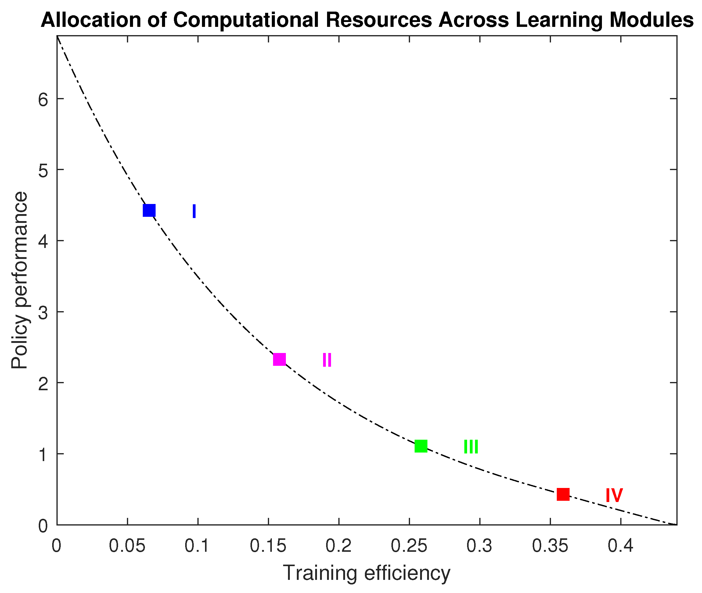
Figure 1 shows the Pareto frontier obtained by the algorithm. Each point corresponds to a non-dominated allocation vector.

5.5. Representative Solutions

From the computed Pareto set, we extract four representative strategies that illustrate different trade-offs between cost and performance (see

Table 1. Representative Pareto-optimal solutions obtained by the proposed method.

Strategy	Cost ${\mathit{f}}_1\left(\mathit{x}\right)$$(\downarrow )$	Performance ${\mathit{f}}_2\left(\mathit{x}\right)$$(\uparrow )$	Interpretation
I	0.92	0.88	High exploration and intensive training; maximizes performance at high computational cost
II	0.65	0.74	Balanced allocation across modules; good trade-off between cost and performance
III	0.43	0.61	Reduced training effort; moderate performance with improved efficiency
IV	0.21	0.45	Minimal resource usage; fast but low-quality policies

).

5.6. Discussion

The numerical results confirm that the proposed method successfully identifies a diverse set of Pareto-optimal solutions. As expected, increasing computational cost leads to improved policy performance, but with diminishing returns.

Compared to naive allocation strategies (e.g., uniform allocation), the proposed approach consistently discovers solutions that dominate baseline configurations. In particular, intermediate strategies (e.g., Strategy II) achieve significant performance gains with moderate computational effort (see Table 1).

5.7. Validation of the Approach

These results demonstrate that:

• The proposed black-box optimization method effectively approximates the Pareto frontier;
• It identifies meaningful trade-offs between conflicting objectives;
• It provides a systematic way to explore resource allocation strategies without requiring explicit knowledge of the underlying model.

Overall, the numerical experiments validate the practical applicability of the approach in complex AI systems where analytical modeling is infeasible.

6. Conclusions and Future Work

In this work, we presented a novel Newton-inspired black-box optimization algorithm for solving multiobjective optimization problems within the framework of ergodic Markov chains, by relying exclusively on function evaluations and derivative approximations—without requiring explicit access to the internal structure of the objective function.

A central contribution of this study is the algorithm’s finite-time convergence guarantee, which strengthens its theoretical foundation while simultaneously improving computational efficiency for driven optimization tasks. The incorporation of an Euler-based approximation scheme further enhances the method’s adaptability and numerical stability, enabling its application to convex systems.

Both the complexity analysis and the numerical experiments confirm the robustness and effectiveness of the proposed approach, demonstrating its ability to deliver high-quality solutions in environments characterized by structural constraints and stochastic dynamics. Overall, this work contributes a practical and theoretically grounded optimization framework that advances the state of the art in optimization, adaptive decision-making, and multiobjective optimization under uncertainty.

Beyond its theoretical significance, the proposed method also exhibits strong practical potential across a range of application domains. In financial engineering, for example, the ability to efficiently optimize portfolio allocations without relying on explicit gradient information is particularly advantageous. The approach provides a scalable and robust alternative to classical optimization techniques. Promising directions for future research include the development of adaptive mechanisms to further accelerate convergence and the extension of the framework to dynamic optimization settings in which objective functions evolve over time.

References

1. Audet, C.; Kokkolaras, M. Blackbox and derivative-free optimization: Theory, algorithms and applications. Optim. Eng. 2016, 17, 1–2. [Google Scholar] [CrossRef]
2. Chen, H.; Zhang, Z.; Li, W.; Liu, Q.; Sun, K.; Fan, D.; Cui, W. Ensemble of surrogates in black-box-type engineering optimization: Recent advances and applications. Expert Syst. Appl. 2024, 248, 123427. [Google Scholar] [CrossRef]
3. Le Besnerais, J.; Fasquelle, A.; Lanfranchi, V.; Hecquet, M.; Brochet, P. Mixed-variable optimal design of induction motors including efficiency, noise and thermal criteria. Optim. Eng. 2011, 12, 55–72. [Google Scholar] [CrossRef]
4. Meo, M.; Zumpano, G. Damage assessment on plate-like structures using a global-local optimization approach. Optim. Eng. 2008, 9, 161–177. [Google Scholar] [CrossRef]
5. Madsen, J.I.; Langthjem, M. Multifidelity response surface approximations for the optimum design of diffuser flows. Optim. Eng. 2001, 2, 453–468. [Google Scholar] [CrossRef]
6. Olivero, M.; Pasquale, D.; Ghidoni, A.; Rebay, S. Three-dimensional turbulent optimization of vaned diffusers for centrifugal compressors based on metamodel-assisted genetic algorithms. Optim. Eng. 2014, 15, 973–992. [Google Scholar] [CrossRef]
7. Martelli, E.; Amaldi, E. PGS-COM: A hybrid method for constrained non-smooth black-box optimization problems: Brief review, novel algorithm and comparative evaluation. Comput. Chem. Eng. 2014, 63, 108–139. [Google Scholar] [CrossRef]
8. Zaryab, S.A.; Scaccabarozzi, R.; Martelli, E. Advanced part-load control strategies for the Allam cycle. Appl. Therm. Eng. 2020, 168, 114822. [Google Scholar] [CrossRef]
9. Peeters, J.; Louarroudi, E.; Bogaerts, B.; Sels, S.; Dirckx, J.; Steenackers, G. Active thermography setup updating for NDE: A comparative study of regression techniques and optimisation routines with high contrast parameter influences for thermal problems. Optim. Eng. 2018, 19, 163–185. [Google Scholar] [CrossRef]
10. Lobanov, A.; Bashirov, N.; Gasnikov, A. The black-box optimization problem: Zero-order accelerated stochastic method via kernel approximation. J. Optim. Theory Appl. 2024, 203, 2451–2486. [Google Scholar] [CrossRef]
11. Feng, Y.; Chen, J.; Pan, T.; Su, R. Rethinking robustness: Robust adversarial distillation for practical black-box signal attack in intelligent fault diagnosis. Expert Syst. Appl. 2025, 294, 128805. [Google Scholar] [CrossRef]
12. Lee, Y.S.; Yen, S.J.; Jiang, W.; Chen, J.; Chang, C.Y. Illuminating the black box: An interpretable machine learning based on ensemble trees. Expert Syst. Appl. 2025, 272, 126720. [Google Scholar] [CrossRef]
13. Ran, Y.; Zhang, A.X.; Li, M.; Tang, W.; Wang, Y.G. Black-box adversarial attacks against image quality assessment models. Expert Syst. Appl. 2025, 260, 125415. [Google Scholar] [CrossRef]
14. Grenier, E.; Helbert, C.; Louvet, V.; Samson, A.; Vigneaux, P. Population parametrization of costly black box models using iterations between SAEM algorithm and kriging. Comput. Appl. Math. 2018, 37, 161–173. [Google Scholar] [CrossRef]
15. Abramson, M.A.; Asaki, T.J.; Dennis, J.E.; O’Reilly, K.R.; Pingel, R.L. Quantitative Object Reconstruction Using Abel Transform X-Ray Tomography and Mixed Variable Optimization. SIAM J. Imaging Sci. 2008, 1, 322–342. [Google Scholar] [CrossRef]
16. Deming, S.N.; Jr, L.R.P.; Denton, M.B. A Review of Simplex Optimization in Analytical Chemistry. Crit. Rev. Anal. Chem. 1978, 7, 187–202. [Google Scholar] [CrossRef]
17. Gray, G.A.; Kolda, T.G.; Sale, K.; Young, M.M. Optimizing an empirical scoring function for transmembrane protein structure determination. INFORMS J. Comput. 2004, 16, 406–418. [Google Scholar] [CrossRef][Green Version]
18. Marsden, A.L.; Feinstein, J.A.; Taylor, C.A. A computational framework for derivative-free optimization of cardiovascular geometries. Comput. Methods Appl. Mech. Eng. 2008, 197, 1890–1905. [Google Scholar] [CrossRef]
19. Oeuvray, R. Trust-Region Methods Based on Radial Basis Functions with Application to Biomedicalimaging. Ph.D. Thesis, Institute of Mathematics, Swiss Federal Institute of Technology, Lausanne, Switzerland, 2005. [Google Scholar]
20. Audet, C.; Béchard, V.; Chaouki, J. Spent potliner treatment process optimization using a MADS algorithm. Optim. Eng. 2008, 9, 143–160. [Google Scholar] [CrossRef]
21. Bartholomew-Biggs, M.C.; Parkhurst, S.C.; Wilson, S.P. Using DIRECT to solve an aircraft routing problem. Comput. Optim. Appl. 2002, 21, 311–323. [Google Scholar] [CrossRef]
22. Fowler, K.R.; Reese, J.P.; Kees, C.E.; Dennis, J.E., Jr.; Kelley, C.T.; Miller, C.T.; Audet, C.; Booker, A.J.; Couture, G.; Darwin, R.W.; et al. Comparison of derivative-free optimization methods for groundwater supply and hydraulic capture community problems. Adv. Water Resour. 2008, 31, 743–757. [Google Scholar] [CrossRef]
23. Spendley, W.; Hext, G.R.; Himsworth, F.R. Sequential application of simplex designs in optimisation and evolutionary operation. Technometrics 1962, 4, 441–461. [Google Scholar] [CrossRef]
24. Nelder, J.A.; Mead, R. A simplex method for function minimization. Comput. J. 1965, 7, 308–313. [Google Scholar] [CrossRef]
25. Hooke, R.; Jeeves, T.A. “Direct Search” Solution of Numerical and Statistical Problems. J. ACM (JACM) 1961, 8, 212–229. [Google Scholar] [CrossRef]
26. Kolda, T.G.; Lewis, R.M.; Torczon, V. Optimization by direct search: New perspectives on some classical and modern methods. SIAM Rev. 2003, 45, 385–482. [Google Scholar] [CrossRef]
27. Conn, A.R.; Scheinberg, K.; Vicente, L.N. Introduction to Derivative-Free Optimization; SIAM: Philadelphia, PA, USA, 2009. [Google Scholar]
28. Clempner, J.B.; Poznyak, A.S. Optimization and Games for Controllable Markov Chains: Numerical Methods with Application to Finance and Engineering; Springer Nature: Cham, Switzerland, 2023. [Google Scholar]
29. Germeyer, Y.B. Introduction to the Theory of Operations Research; Nauka: Moscow, Russia, 1971. [Google Scholar]
30. Clempner, J.B. Necessary and Sufficient Karush-Kuhn-Tucker Conditions for Multiobjective Markov Chains Optimality. Automatica 2016, 71, 135–142. [Google Scholar] [CrossRef]
31. Clempner, J.B.; Poznyak, A.S. Constructing The Pareto Front For Multiobjective Markov Chains Handling A Strong Pareto Policy Approach. Comput. Appl. Math. 2018, 37, 567–591. [Google Scholar] [CrossRef]
32. Clempner, J.B.; Poznyak, A.S. A Tikhonov Regularization Parameter Approach For Solving Lagrange Constrained Optimization Problems. Eng. Optim. 2018, 50, 1996–2012. [Google Scholar] [CrossRef]
33. Clempner, J.B.; Poznyak, A.S. Multiobjective Markov chains optimization problem with strong Pareto frontier: Principles of decision making. Expert Syst. Appl. 2017, 68, 123–135. [Google Scholar] [CrossRef]
34. Kesten, H. Accelerated stochastic approximation. In The Annals of Mathematical Statistics; Institute of Mathematical Statistics: Waite Hill, OH, USA, 1958; pp. 41–59. [Google Scholar]
35. Spruill, M.; Studden, W. A Kiefer-Wolfowitz theorem in a stochastic process setting. In The Annals of Statistics; Institute of Mathematical Statistics: Waite Hill, OH, USA, 1979; pp. 1329–1332. [Google Scholar]
36. Broadie, M.; Cicek, D.; Zeevi, A. General bounds and finite-time improvement for the Kiefer-Wolfowitz stochastic approximation algorithm. Oper. Res. 2011, 59, 1211–1224. [Google Scholar] [CrossRef]
Figure 1. Approximated Pareto frontier obtained via black-box optimization.
Mca 31 00063 g001