An Evaluation of Supervised Machine Learning Pipelines for the Identification of Distributed Denial-of-Service Attacks Using Conventional and Computational Performance Metrics

Abstract

Distributed denial-of-service (DDoS) attacks, a type of Denial-of-Service (DoS) attack in which the targeted server, service or network is overloaded with malicious traffic originating from various different sources with the aim of making such targets inaccessible for legitimate users, continue to pose a pertinent threat to the availability and integrity of organisational digital assets. While many studies have shown that machine learning models can provide high predictive accuracy in detecting such attacks, they often fail to evaluate the practicality of deploying such models to production. This study aims to address this gap by evaluating a considerable amount of pipelines based on five popular supervised classifiers for detecting DDoS attacks using the CICDDoS2019 dataset. The study employs a comprehensive methodology that combines both manual feature removal with automated encoding, scaling and feature selection integrated within pipelines. A total of 210 pipelines formed of five classifiers, three features selectors, two hyperparameter tuners and seven train–test splits were initially evaluated. Pipeline performance was assessed using both conventional and computational performance metrics. To identify the champion pipeline, a two-step approach was employed: composite scoring for shortlisting and statistical testing using Friedman and post hoc Nemenyi tests. The champion pipeline was shown to be Decision Tree coupled with Recursive Feature Elimination (with 20 features selected) and Grid Search hyperparameter tuning with a 90-10 train–test split. It achieved the most optimal balance of predictive capabilities and computational overheads, achieving an MCC of $0.993\pm 0.024$, training time of $0.194\pm 0.001$ s, inference time of $0.000998\pm 0.00008$ s, CPU time of $0.194\pm 0.008$ s and average memory usage of 15,167 ± 322 kilobytes across training and inference. The findings highlight the importance of a holistic and more nuanced approach when selecting a champion pipeline that is not only effective but also feasible for deployment in resource-constrained environments.

1. Introduction

As global connectivity continues to grow, with over two thirds of the world’s population now having access to the Internet [1], the challenges that come with DDoS attacks are further compounded by the emergence of cybercrime-as-a-service models. In particular, DDoS-as-a-service operations (aka. DDoS for hire), which have become even more prevalent due to the increase in the commercialisation of cybercrime [2,3]. DDoS-as-a-service operations enable low-skilled adversaries to carry out powerful DDoS attacks against any potential targets for an often minimal fee [4,5]. As a result, traditional detection methodologies are often insufficient when dealing with modern DDoS attacks, underscoring the desperate need for more intelligent approaches. Researchers and companies alike are turning to the use of artificial intelligence and more specifically machine learning (ML) to solve the DDoS problem, with some real-world solutions already in production.

While the literature continues to propose numerous ML models as viable solutions for detecting DDoS attacks, there has been a noticeable lack of discussion and assessment of their practical feasibility. Most studies evaluate models solely using conventional metrics such as accuracy, precision, recall and F1-score, although some studies do also go beyond this. While these metrics are often highly useful, they only form a single dimension in the model evaluation process. This is because they do not measure other factors that are of crucial importance in such applications, such as deployment feasibility, scalability, detection speed and resource requirements for model training and testing.

Thus, this study aims to evaluate hundreds of supervised ML pipelines for detecting modern DDoS attacks using the CICDDoS2019 dataset [6]. Specifically, we investigate which pipeline configurations achieve the best of both worlds in terms of predictive accuracy and computational efficiency and identify the features of the CICDDoS2019 dataset that contribute most to effective detection. Additionally, the trade-offs between accuracy and computational efficiency across different pipelines are examined to inform practical deployment of DDoS detection systems. To achieve this, this study is guided by three objectives: (a) to evaluate the performance of hundreds of supervised ML pipelines on the CICDDoS2019 dataset using conventional and computational metrics; (b) to identify the features of the CICDDoS2019 dataset that contribute the most to effective detection; and (c) to assess the trade-offs between predictive accuracy and computational efficiency across different pipeline configurations.

2. Related Work

2.1. Classifiers

Supervised ML has emerged as a widely used ML paradigm for detecting DDoS attacks [7]. This is primarily due to its ability to learn complex patterns from labelled data such as network traffic with ease [7]. Supervised ML models are trained on datasets that contain both benign and malicious traffic. This enables them to classify data points based on learned characteristics that appear in the form of dataset features. In DDoS attack detection, the primary goal of these solutions is to identify malicious traffic quickly and accurately, seeking to enable timely mitigation before services suffer significant impact. A variety of supervised ML algorithms have been explored within the literature; these include Decision Trees (DT), Random Forests (RF), Support Vector Machines (SVM), Naive Bayes (NB) and k-Nearest Neighbour (kNN) [8,9,10,11,12]. Each algorithm has its own strengths and trade-offs. Among the popular choices, tree-based models are favoured for their inherent interpretability and fast training, making them suitable for real-world DDoS detection. Particularly, the dominance of RF in the literature can be attributed to its ability to reduce overfitting through the use of multiple trees and ability to handle highly dimensional data. This is often desired, as most benchmark datasets are highly dimensional. Further, their relatively fast training times making them well-suited for DDoS detection [13].

While supervised ML often achieves high accuracy in controlled environments, such as studies, they face several limitations when it comes to real-world deployment feasibility. The performance of these models is often highly dependent on the availability of high-quality and up-to-date labelled datasets, which can be particularly difficult to obtain given both the rapid evolution of DDoS attacks in modern times but also the privacy concerns related to sharing such sensitive data, as is the case with network traffic. Furthermore, the very nature of supervised ML provides a limitation that manifests in requiring frequent updates to the training data as well as retraining to remain effective against novel or zero-day attack patterns, which models do not see during training. Finally, prior works have typically explored a relatively small number of classifiers, feature selectors, hyperparameter tuners and train–test splits, if any.

Despite these limitations, supervised ML remains an integral component of modern DDoS detection systems, especially when proper feature engineering, dataset selection and curation, and hyperparameter tuning takes place. As prior works have shown, RF’s combination of accuracy and interpretability makes it particularly suited for DDoS detection.

2.2. Data Sources

The choice of dataset significantly impacts the performance and generalisability of ML models, thus the selection of the dataset used in this study is crucial [14]. Several benchmark datasets are commonly used in DDoS detection research (see

Table 1. Popular datasets used within the DDoS attack detection literature.

Name	Year	Source
KDD99 [15]	1999	Defense Advanced Research Projects Agency (DARPA)
NSL-KDD [16]	2009	University of New Brunswick (UNB) and Canadian Institute for Cybersecurity (CIC)
UNSW-NB15 [17]	2015	University of New South Wales (UNSW)
CIC-IDS2017 [18]	2017	University of New Brunswick (UNB) and Canadian Institute for Cybersecurity (CIC)
CIC-DDoS2019 [6]	2019	University of New Brunswick (UNB) and Canadian Institute for Cybersecurity (CIC)

), each with distinct strengths and limitations. KDD99 [15] and its updated version NSL-KDD [16] have been widely used due to their age and reputation. However, their outdated traffic patterns reduce their relevance significantly for DDoS detection in the modern day [17]. To address this, UNSW-NB15 [17] and CIC-IDS2017 [18] provide more realistic network traffic and richer feature sets, improving model performance, though neither is specifically focused on DDoS attacks. CIC-DDoS2019 [6] directly focuses on DDoS attacks, covering many different attack vectors. Despite its imbalance, it remains the most comprehensive, popular, publicly available dataset for evaluating ML models for DDoS detection. Further, certain datasets are purely synthetic; that is, they contain data that are artificially generated using tools rather than produced by real events, while other datasets rely on controlled test environments that, despite being much more realistic, may still not fully capture the true nuances of modern networks [19]. Additionally, some of these datasets suffer from class imbalance and being out of date [20]. Thus, these differences directly influence the generalisability of supervised classifiers that are trained on them as they may learn patterns that do not directly translate well into real-world DDoS attack scenarios.

2.3. Pre-Processing, Feature Selection and Model Evaluation

Pre-processing steps are often important for multiple reasons; notably, scaling must be applied when using distance-based classifiers such as SVM. Moreover, balancing is needed due to class imbalances. Some of the commonly utilised pre-processing steps include scaling, normalisation, and encoding. Feature selection is also often a key component in supervised ML pipelines. Some of the commonly used families of feature selectors include filter-based, wrapper-based and embedded methods. This is often a key step in ML as datasets can have redundant or highly correlated features that can hinder performance [21,22]. Prior studies often only applied a single feature selector that was directly tailored to the problem using expert knowledge and did not compare different selectors conclusively.

Model evaluation within the context of DDoS detection and supervised ML more broadly typically involves metrics such as accuracy, precision, recall and F1-score [23]. These, however, often do not capture the full performance spectrum of a given model or pipeline. Despite this lack of holistic perspective, the conventional metrics that are used also have their inherent issues. For example, when datasets are imbalanced, the use of accuracy as a primary or target metric can be often be misleading [24], as a model with high accuracy may just be favouring the majority class, and thus fail to detect the minority class. As a result, many studies report and utilise precision and recall to provide a more accurate perspective on model performance in these scenarios. Furthermore, depending on the specific situation, either metric may be far more important than the accuracy. For example, failing to detect a critical cyberattack such as a DDoS attack can result in a costly impact [25], meaning that recall is often a crucial metric in DDoS detection studies. Similarly, causing unnecessary false alarms is also a significant problem as it can degrade the response from technical users due to a phenomenon known as alert fatigue [26]. The F1-score is thus used as it provides a balance between precision and recall, allowing for the best of both worlds. While these four conventional metrics dominate the literature in terms of model evaluation, some studies do also explore additional or different metrics such as ROC-AUC to offer deeper insights into model performance [27]. Despite the importance of accurately detecting cyberattacks as impactful as DDoS attacks, relatively few studies explore model performance from a computational efficiency standpoint.

3. Materials and Methods

3.1. Study Design

This paper adopts a quantitive–experimental approach that utilises the well-known benchmark dataset CICDDoS2019 to both train and evaluate hundreds of different supervised ML pipelines across a set of conventional and computational evaluation metrics. The primary aim is to assess which supervised ML pipeline is the most effective at both accurately and efficiently identifying malicious network traffic. To ensure a fair and comprehensive comparison and evaluation, all of the pipelines created as part of this study were trained and evaluated on the same pre-processed dataset using the same evaluation metrics and run on the same hardware. Numerous feature selection and hyperparameter tuning approaches were also assessed to identify which combination of approaches provides the best trade-off between performance and computational overhead. The quantitive nature of this study will enable it to ensure that any conclusions drawn regarding the efficacy of any pipelines remain data-driven, sound and verifiable.

3.2. Dataset

The basis of this study is the CIC-DDoS2019 dataset [6]. It is a publicly accessible dataset often utilised for benchmarking intrusion detection systems, with a specific focus on DDoS attacks. The dataset was created by the Canadian Institute for Cybersecurity in collaboration with the University of New Brunswick in 2019 and is a widely recognised and adopted dataset within the literature due to its comprehensive, labelled nature and realistic representation of modern network traffic and attack patterns [6]. The dataset is structured as a collection of 18 individual CSV files separated by the type of DDoS attack performed and then further divided into training and testing folders that were collected at different times. Once merged, the dataset comprises a total of 70,427,637 records, with 70,313,809 records being labelled as various DDoS attack types, with the remaining 113,828 records being benign traffic [28]. The dataset is highly imbalanced, with 99% of records being labelled as malicious. The dataset also contains 87 unique features, with 80 being of statistical nature, extracted using the CICFlowMeter tool [29], and the remaining 7 features being socket- or metadata-related information (i.e., Flow ID, Source IP, Protocol or Timestamp). The features are a mix of numerical and categorical data, with numerical data being the dominant data type. Further, the features capture a range of different characteristics such as flow duration, packet count and protocol type [30].

3.3. Pre-Processing

Due to the initial structure of the dataset, the data is of a multi-class nature, with each record being labelled according to the DDoS attack that was performed or alternatively as benign traffic. However, for the purpose of this study, these labels were converted into a single attack-specific label called “MALICIOUS” as a binary classification problem was explored, with benign records retaining their original “BENIGN” label.

ML model development often requires a critical step to ensure that the data is refined and of the highest possible quality, this being pre-processing. This step helps to eliminate or reduce any potential noise that may be present in the dataset, and by proxy, helps improve model performance. To enable the experiments to be carried out on the pipelines in a timely manner, a sample of the original dataset was taken; specifically, a sample of roughly 25,000 rows was used (see

Table 2. Number of rows in the dataset by attack type before and after applying the sampling approach.

Attack Type	No. of Rows (Before)	No. of Rows (After)
TFTP	20,107,827	7128
MSSQL	10,300,824	3659
NetBIOS	7,550,885	2750
UDP	6,919,008	2484
SYN	5,903,222	2296
SNMP	5,161,377	1831
DNS	5,074,413	1800
LDAP	4,924,776	1453
SSDP	2,611,374	926
NTP	1,217,007	427
UDPLag	725,165	131
Portmap	191,694	66
Total	70,313,809	24,951

). To obtain the sample, each CSV file from the dataset was proportionally randomly stratified andsampled, to ensure that the sampled dataset retained its original class distribution and its proportional size to each file in the original dataset. A random sample of records was taken from each CSV file and stratified against the target column (Label). The total number of records used was chosen based on the computing resources available.

To prepare the dataset for the pipelines, various data inspection and pre-processing steps were carried out (see Figure 1). First, due to the nature of the dataset, namely where each attack type is given its own label, all the DDoS attack type labels were combined under one over-arching “MALICIOUS” label for completeness and correctness. Second, the data was identified to have missing data within the Flow Bytes/s and SimillarHTTP columns with 93 and 4 rows of missing data respectively. Next, duplicate rows were identified using a filter-condition method; curiously, no duplicate rows were identified. Further, four columns, specifically, Fwd Header Length, min_seg_size_forward, Init_Win_bytes_forward and Init_Win_bytes_backward, were identified to contain negative values, with both Init_Win_bytes_forward and Init_Win_bytes_backward containing in excess of 90% negative values and Fwd Header Length and min_seg_size_forward containing around 12.36% and 15.92% respectively.

Column names were stripped of any white spaces that prepended or appended them. Furthermore, columns that were deemed to be irrelevant based on factors such as high homogeneity, lack of contribution to the model and excessive amounts of invalid data were removed, these were: Row No., Flow ID, Source IP, Destination IP, Protocol, SimillarHTTP, Timestamp, Init_Win_bytes_forward, Init_Win_bytes_backward, Bwd PSH Flags, Fwd URG Flags, Bwd URG Flags, FIN Flag Count, SYN Flag Count, RST Flag Count, PSH Flag Count, URG Flag Count, CWE Flag Count, ECE Flag Count, Fwd Avg Packets/Bulk, Fwd Avg Bytes/Bulk, Fwd Avg Bulk Rate, Bwd Avg Packets/Bulk, Bwd Avg Bytes/Bulk, and Bwd Avg Bulk Rate. As identified during the data inspection, both min_seg_size_forward and Fwd Header Length contained negative values. To resolve this, the rows that contained said negative values were filtered out of the dataset, with min_seg_size_forward being removed first as it contained a higher proportion of negative values. As neither the minimum segment size nor the header length can realistically be a value below zero, it was deemed that the negative values present in these columns were the result of placeholders or logging issues in the tooling that was utilised during data collection. Subsequently, the missing values identified were also handled. Given that SimillarHTTP was dropped due to its irrelevance, the remaining column with missing data, Flow Bytes/s, was handled accordingly, with 93 rows being dropped from the dataset. Similarly, infinite values in both Flow Bytes/s and Flow Packets/s were also dropped, resulting in 20,304 rows and 62 columns remaining after pre-processing. Outliers were not handled explicitly as RobustScaler was used instead. The model evaluation loop also features the use of LabelEncoder which ensures that the class labels are appropriately encoded. Data quality checks were performed after each significant pre-processing step using the helper function check_data_quality, which noted the shape (rows and columns) along with the number of missing values and duplicate rows.

Table 3. Dataset shape, missing value count and duplicate row count before and after each pre-processing stage.

Stage	Shape	No. of Missing Values	No. of Duplicate Rows
Unprocessed Data	(24,992, 88)	97	0
Data Pruning	(21,013, 63)	93	0
Data Wrangling	(20,304, 63)	0	0
Deduplication	(20,304, 62)	0	0
Final	(20,304, 62)	0	0

shows the dataset shape, missing value count and duplicate row count before and after each pre-processing stage, while

Table 4. Number of rows in the dataset by class before and after pre-processing.

Class	No. of Rows (Before)	No. of Rows (After)
BENIGN	41	39
MALICIOUS	24,951	20,265
Total	24,992	20,304

shows the number of rows in the dataset by class before and after the pre-processing step.

3.4. Evaluation Metrics

Evaluation metrics are used to assess the performance of the supervised machine learning pipelines explored in this study. The reason for such metrics is that without them, evaluation and comparison of pipelines cannot be performed, and thus, the pipelines are not grounded in reality [31]. This study makes use of five popular metrics: accuracy, precision, recall, F1-score and Matthews Correlation Coefficient (MCC). Equations (1)–(4) show how they were calculated.

$$Accuracy={\displaystyle \frac{TP+TN}{TP+TN+FP+FN}}$$

(1)

$$Precision={\displaystyle \frac{TP}{TP+FP}}$$

(2)

$$Recall={\displaystyle \frac{TP}{TP+FN}}$$

(3)

$$F1\_score={\displaystyle \frac{2·Precision·Recall}{Precision+Recall}}$$

(4)

$$MCC={\displaystyle \frac{TP·TN-FP·FN}{\sqrt{(TP+FP)(TP+FN)(TN+FP)(TN+FN)}}}$$

(5)

where TP, FP, TN, and FN represent true positives, false positives, true negatives, and false negatives, repsectively.

Additionally, four computational metrics were used:training time, inference time (batch inference), CPU time and average memory usage (see Algorithms A1–A4). Reporting these metrics is essential for evaluating not only the predictive capabilities but also the computational efficiency of the pipelines, especially when considering their practicality in real-world scenarios. In certain applications of ML, especially those in resource-constrained environments, an understanding of computational costs is critical for ideal pipeline selection, as a balance of good predictive performance and low computational cost is often required. The use of these metrics aims to provide some insight into the potential scalability and deployment feasibility of each pipeline in a modern network.

3.5. Models

This study makes use of several supervised machine learning classifiers, including Logistic Regression (LR), Support Vector Machine (SVM) [32], Decision Tree (DT) [33], Random Forest (RF) [34] and Extreme Gradient Boost (XGBoost) [35] in a binary classification scenario. All of these classifiers are supervised classifiers and thus are trained on labelled data, such that they can learn the mapping between the input features and the labels. These classifiers were selected due to their widespread adoption within the literature as well as their diversity across different model families. LR is a linear-based probabilistic classifier that models the probability of a data point belonging to one of two classes. SVM is a margin-based classifier that aims to identify the most optimal decision boundary such that class separation is maximised. DT is a rule-based tree-structured classifier that makes decisions based on a dataset’s features using multiple if–then splits until it identifies a split path that yields the most optimal split. RF is an ensemble classifier made up of multiple decision trees, which aids in improving performance and reduces the overfitting experienced by decision trees. While XGBoost is also an ensemble classifier, it is based on gradient boosting, where multiple decision trees are built sequentially, with each new tree focusing on correcting the errors of the previous ones.

3.6. Experimental Setup

The pipelines were executed in a controlled environment to ensure both consistency and reproducibility across all explored pipeline configurations. The environment consisted of a desktop computer with an AMD Ryzen 7 7800X3D CPU rated at 4.20 GHz with 8 cores and 16 threads; 32 GBs of DDR5 RAM; Windows 11 Pro 64-bit as the operating system and Python version 3.13.6. The code developed as part of this study was implemented using Python. All of the code development took place on a Jupyter Notebook with several key libraries used, which were numpy 2.3.2, pandas 2.3.1, polars 1.32.3, scikit-learn 1.7.1, matplotlib 3.10.5, jupyterlab 4.4.5, xgboost 3.0.4, pyarrow 20.0.0, shap 0.51.0, scikit-posthocs 0.12.0 and requests 2.32.4. To maintain code quality and consistency, all of the code was developed in adherence with the Google Python Style Guide. All classifiers explored in this study were trained without the use of GPU acceleration. To monitor both the average and peak memory usage during training and inference, a custom profiler was implemented that sampled the process’ memory approximately every 100 ms (0.1s) in a separate thread (see Appendix A Algorithm A4). This approach aimed to provide a balance between measurement overhead and resolution, capturing sustained memory peaks and trends while avoiding any interference with the pipeline’s execution.

In order to streamline model development, scikit-learn pipelines were employed through the use of the Pipeline interface. This interface enables the encapsulation of multiple different pipeline components into a single reproducible object, making it particularly useful in machine learning workflows that involve a fixed sequence of steps [36]. Each pipeline explored comprised three key stages: feature selection, hyperparameter tuning and classification. In the feature selection stage, the dimensionality of the dataset was reduced to improve the performance of each model; specifically, the SelectKBest, VarianceThreshold and RFE functions were used due to their availability. SelectKBest is a filter-based feature selection technique that ranks features using univariate statistical tests and retains the top-k most relevant features. VarianceThreshold is also a filter-based feature selection technique, but instead, it removes all features whose variance does not meet the defined threshold. Finally, RFE is a wrapper-based feature selection technique that repeatedly trains and evaluates a machine learning model on different subsets of features with the least important features being pruned from the original set until the desired number of features is reached.

Hyperparameter tuning was implemented through the use of the GridSearchCV and RandomizedSearchCV functions. Train–test split ratios were pre-computed with random_state=42 and stored in a dictionary for easy retrieval within the model evaluation loop when needed. A summary of all pipeline components explored in this study is provided in

Table 5. Pipeline configuration options that were explored in the study.

Component	Options
Feature Selection (FS)	SelectKBest, VarianceThreshold and RFE
Hyperparameter Tuning (HT)	GridSearchCV and RandomizedSearchCV
Train–Test Ratios (TTR)	90-10, 85-15, 80-20, 75-25, 70-30, 65-35, 60-40

. Despite the fact that a larger and more expansive hyperparameter grid may have provided much more complex insights, due to computational limitations and other constraints, the scope of the hyperparameter grids was narrowed by prioritising parameters and values that were most likely to yield meaningful results. The selection of parameter values hinged on retaining enough variation to allow for robust comparisons without significantly impacting computational demands (see

Table 6. Parameter grids used for classification algorithms and feature selection methods in this study.

Classifier	Options
Random Forest	n_estimators: [100, 200] max_depth: [1, 5, 10] max_features: [’sqrt’, ’log2’]
Decision Tree	max_depth: [1, 5, 10] criterion: [’gini’, ’entropy’]
Support Vector Machine	C: [0.1, 1]
Extreme Gradient Boosting	learning_rate: [0.01, 0.1] max_depth: [2, 3] max_leaves: [2, 3]
Logistic Regression	C: [0.001, 0.01, 0.1] (solver = ’sag’, max_iter = 20,000, random_state = 42)
Selector	Options
SelectKBest	k: [10, 20] score_func: [f_classif, mutual_info_classif]
VarianceThreshold	threshold: [0.1, 0.5, 1.0]
RFE	n_features_to_select: [10, 20] (estimator = DecisionTreeClassifier(), step = 6)

). Ultimately, the trade-off between search space coverage and computing time was necessary to obtain results in an appropriate amount of time.

4. Results and Discussion

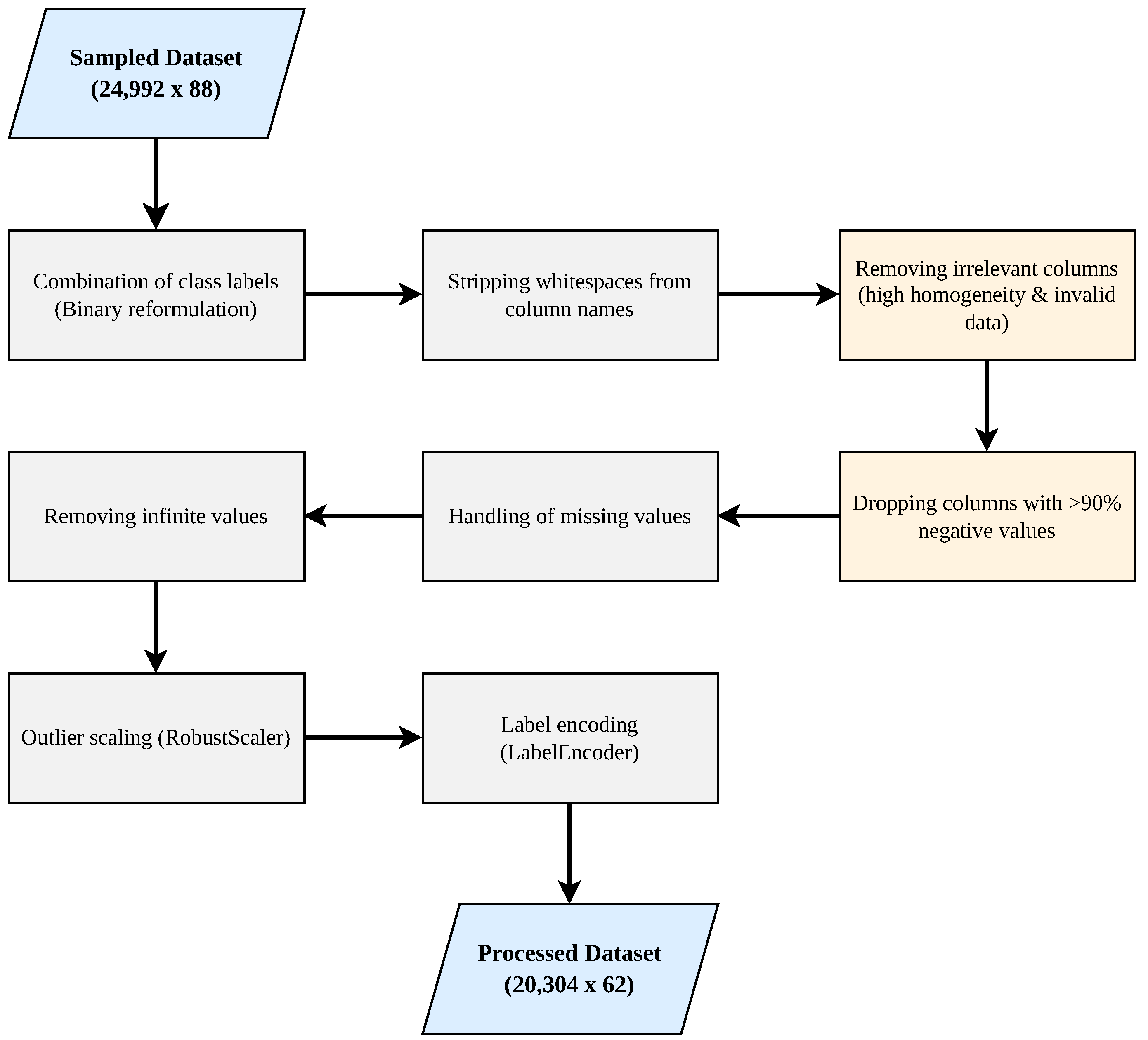
The findings from this study’s evaluation of a variety of supervised machine learning pipeline configurations for DDoS attack detection using the CICDDoS2019 dataset are discussed in this section. Additionally, statistical testing, feature importance analysis and generalisation evaluation are performed to strengthen the findings. The primary objective was to investigate the most effective pipeline configuration by systematically evaluating and assessing their performance across a range of conventional and computational metrics. The study involved a total of 210 unique pipelines that comprised five supervised classifiers, three feature selection techniques, two hyperparameter tuning techniques and seven train–test splits and were evaluated using nine metrics: accuracy, precision, recall, F1, MCC, training time, inference time, average memory usage and average CPU time. The following section will detail the performance results starting from a wider perspective, then it will hone in on the top 10 most performant pipelines; subsequently, feature frequency analysis is performed to identify the most effective features for detection, and finally the section concludes with a discussion of performance trade-offs. The metric values were obtained by training and evaluating each pipeline against the same pre-processed dataset that was stratified and randomly sampled from the original dataset, containing a total of 20,304 rows and 62 columns (61 features, 1 label) post pre-processing.

4.1. Performance Results

Generally, as shown in

Table 7. Comparison of classifiers across all pipelines with key metrics averaged and reported.

Classifier	Avg. MCC	Avg. Training Time	Avg. Inference Time	Avg. CPU Time	Avg. Memory Usage
RF	0.78936	13.35667	0.01014	1.315	1979
DT	0.73702	3.65117	0.00206	0.263	1388
XGBoost	0.62434	6.09475	0.00309	1.570	2547
SVM	0.06931	2.97831	0.02476	0.805	4304
LR	0.06062	88.29600	0.00227	15.637	1605

, pipelines that utilise tree-based classifiers dominate predictive performance. LR-based pipelines appear to struggle, suggesting that there may be non-linear patterns in the data that they simply are not able to catch, or that the interactions between features in the dataset cannot be effectively captured by linear models. Further, LR-based pipelines also have considerably higher training times compared to other pipelines; this, however, may be the result of having to provide static parameters to the LR classifier function from scikit-learn to enable it to identify a valid model within the max_iter limit. SVM and DT both exhibit very fast training times compared to more complex models such as XGBoost and RF. Similarly, DT-based pipelines note the fastest inference times on average. Additionally, DT-based pipelines also showcase the lowest memory usage on average, indicating that they are more memory-efficient in comparison to other classifiers. On the other hand, SVM showcases the worst memory usage, likely due to its need to store the generated support vectors.

As shown in

Table 8. Comparison of feature selectors across all pipelines with key metrics averaged and reported.

Feature Selector	Avg. MCC	Avg. Training Time	Avg. Inference Time	Avg. CPU Time	Avg. Memory Usage
SelectKBest	0.51649	25.39273	0.00636	3.867	2840
RFE	0.45046	11.41038	0.00744	2.239	2103
VarianceThreshold	0.40144	31.82303	0.01159	5.647	2151

, feature selection results highlight that SelectKBest offers the highest predictive performance with an MCC of 0.51649, at the clear cost of more memory usage and a moderate increase in training time compared to RFE, making it the most suitable and practical selector for maximising predictive performance. RFE achieves moderately lower predictive performance with an MCC of 0.45046, but it is both faster in training time and more memory-efficient, showcasing a good compromise between computational resources and predictive performance on average when needed. VarianceThreshold performs the worst across the predictive performance metric and most computational metrics, indicating that it is likely not an appropriate selector for the CICDDoS2019 dataset because of the feature complexity present within in the dataset.

Comparing both hyperparameter tuning methods explored in this study shows a clear trade-off between predictive performance and computational efficiency (see

Table 9. Comparison of hyperparameter tuning techniques across all pipelines with key metrics averaged and reported.

Tuner	Avg. MCC	Avg. Training Time	Avg. Inference Time	Avg. CPU Time	Avg. Memory Usage
Grid	0.50017	33.35423	0.00835	3.996	1547
Random	0.41209	12.39653	0.00858	3.840	3182

). The Grid tuner achieves a higher average MCC score (0.50017) compared to the Random tuner (0.41209), indicating better overall performance. However, despite this, it comes at the cost of significantly longer training times, with Grid taking an average of 33.35 s versus only 12.40 s for Random. In terms of inference time, both methods perform similarly (roughly 0.008 s), suggesting that prediction speed is largely unaffected by the tuning method employed in the pipeline. The CPU time is also comparable across the tuners, with Random being slightly lower. On the other hand, Random tuning appears to consume slightly over two times more memory than Grid tuning on average. Overall, while Grid tuning provides better predictive performance and lower memory usage on average, it still requires substantially more training time, whereas Random tuning sacrifices some predictive performance and uses memory to achieve faster training speeds.

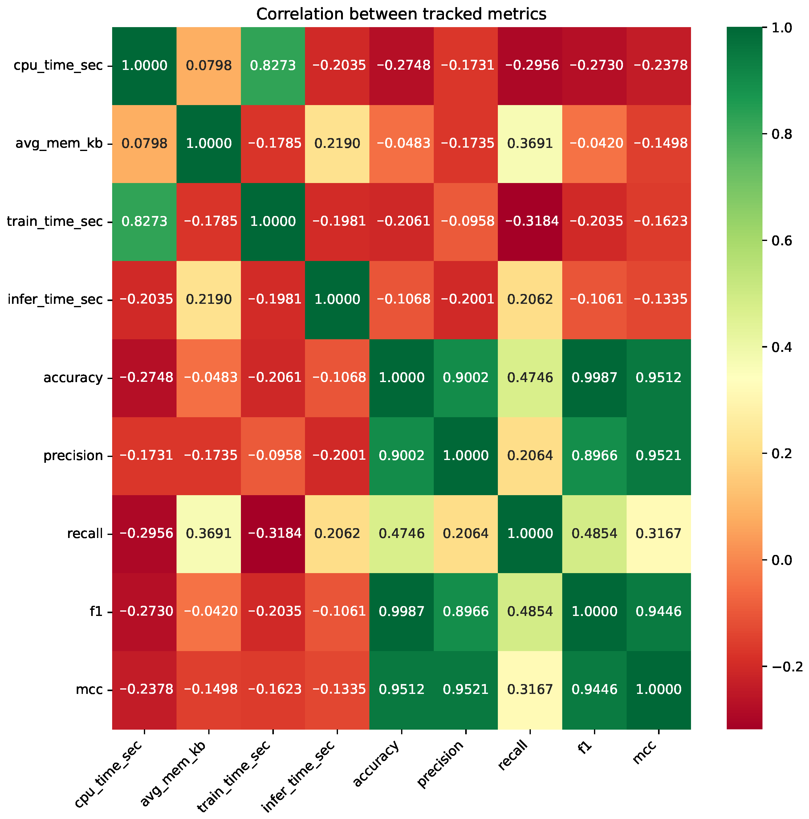
To identify the champion pipeline from the 210 that were evaluated in this study, a two-step approach was used: composite scoring and statistical testing. First, composite scoring was employed. To do this, we identified, using Spearman’s correlation coefficient, highly correlated metrics such as accuracy, recall, precision and F1 and removed them from the composite scoring formula to avoid redundant contributions (see Figure 2). This formula was used to ensure that each metric reflected some form of unique information about the pipeline itself, rather than overweighting a specific aspect, where $x_{ij}^{\mathrm{norm}}$ is the normalised metric and $w_j$ is its weight (see Equation (6)). Despite train_time_sec and cpu_time_sec being highly correlated with each other ($r=0.8273$) they were both retained, as they capture distinct aspects of the computational efficiency of a given pipeline. Moreover, to not overweight them, their combined influence was controlled through a weight for each metric of 0.125. Next, each metric was normalised to a range of [0, 1] based on whether higher values were indicative of better (e.g., MCC) or worse (e.g., training time) performance (see Equation (7)). This weighted composite score was computed from the normalised metrics to produce a preliminary ranking of the top 10 candidate champion pipelines. The top 10 pipelines presented in

Table 10. Pipelines ranked by composite score with top 10 reported.

Pipeline	Composite Score
DT_VarianceThreshold_Grid_90-10	0.980111
RF_RFE_Grid_85-15	0.961469
DT_RFE_Grid_90-10	0.959835
DT_RFE_Grid_85-15	0.959645
RF_RFE_Grid_80-20	0.957575
DT_RFE_Grid_80-20	0.954237
RF_RFE_Grid_90-10	0.947317
DT_VarianceThreshold_Grid_75-25	0.939987
XGBoost_VarianceThreshold_Grid_85-15	0.935331
DT_SelectKBest_Grid_90-10	0.933228

were selected according to this weighted composite score.

$$\mathrm{Composite}{\mathrm{Score}}_i=\sum _{j=1}^M{w}_j·x_{ij}^{\mathrm{norm}}$$

(6)

$$x_{\mathrm{norm}}=\left\{\begin{array}{cc}{\displaystyle \frac{x-x_{min}}{x_{max}-x_{min}}},\hfill & \mathrm{if}\mathrm{higher}\mathrm{is}\mathrm{better}\hfill \\ {\displaystyle \frac{x_{max}-x}{x_{max}-x_{min}}},\hfill & \mathrm{if}\mathrm{lower}\mathrm{is}\mathrm{better}\hfill \end{array}\right.$$

(7)

Second, statistical testing was performed on the top 10 selected pipelines, with each candidate pipeline being re-run 10 times with a different random_seed value set for the train_test_split function each time, generating multiple measures for each metric. These repeated measures enabled the use of the Friedman test to assess whether the performance differences among the top 10 pipelines’ metrics were statistically significant. For each of the 9 metrics, the Friedman test was applied to determine if any pipeline performed significantly differently from the others. When the test indicated significance ($p<0.05$), a post hoc Nemenyi test was used to identify which pipelines differed significantly in pairwise comparisons, the results of which are summarised in

Table 11. Top-performing pipelines for each predictive metric. An X indicates a pipeline identified as top-performing by the Nemenyi post hoc tests.

Pipeline	MCC	F1	Accuracy	Precision	Recall
DT_RFE_Grid_90-10	X	X	X	X	X
DT_VarianceThreshold_Grid_90-10
DT_SelectKBest_Grid_90-10					X
DT_RFE_Grid_85-15	X	X	X	X	X
DT_RFE_Grid_80-20	X	X	X	X	X
DT_VarianceThreshold_Grid_75-25
RF_RFE_Grid_90-10					X
RF_RFE_Grid_80-20					X
RF_RFE_Grid_85-15	X		X	X	X
XGBoost_VarianceThreshold_Grid_85-15

and 

Table 12. Top-performing pipelines for each computational metric. An X indicates a pipeline identified as top-performing by the Nemenyi post hoc tests.

Pipeline	CPU Time	Avg. Mem Usage	Training Time	Inference Time
DT_RFE_Grid_90-10				X
DT_VarianceThreshold_Grid_90-10
DT_SelectKBest_Grid_90-10			X
DT_RFE_Grid_85-15
DT_RFE_Grid_80-20
DT_VarianceThreshold_Grid_75-25	X
RF_RFE_Grid_90-10		X
RF_RFE_Grid_80-20
RF_RFE_Grid_85-15
XGBoost_VarianceThreshold_Grid_85-15

.

Despite the post hoc tests not being able to identify a single statistically superior pipeline across all of the metrics, they still revealed notable differences in specific pairwise comparisons. Several of the pairwise comparisons highlighted meaningful differences between specific pipelines, revealing trends that are not immediately apparent. While several pipelines excel in specific metrics, no single pipeline dominates across all of them, highlighting the trade-offs between computational efficiency and predictive performance. Thus, with Table 11 and Table 12 (where an X character denotes a top-performing pipeline for a given metric) in mind, the selection of the champion pipeline is based on choosing the pipeline that is top-ranked in a majority of metrics rather than strict statistical superiority. As a result, DT_RFE_Grid_90-10 was identified to be the champion pipeline, ranking highest across six of the nine metrics considered, Recall, Precision, Accuracy, F1, MCC and Inference Time, with other pipelines not achieving the same.

With the champion pipeline, the false negative rate (FNR) achieved was 0, indicating that no positive samples were misclassified (see

Table 13. Confusion matrix of champion pipeline (DT_RFE_Grid_90-10).

Actual/Predicted	Positive	Negative
Positive	TP = 2026	FN = 0
Negative	FP = 0	TN = 5

). However, given the relative size of the negative class (n = 5), the conventional performance metrics are highly sensitive to individual misclassifications. Consequently, while the pipeline appears to perfectly avoid false positives and false negatives, the results should be interpreted with caution. The observed performance may overstate the pipeline’s robustness and may not generalise well to other datasets with a larger size or more balanced class distribution.

In real-world applications where negative samples are much more abundant, even a small number of false positives may reduce precision and increase operational costs, such as allocating resources like analysts to inspect flagged events. The limited test size also raises the risk that the pipeline is overfitted to CIC-DDoS2019, meaning that its apparent perfect performance may not hold in cross-dataset evaluations.

4.2. Feature Analysis

From the top 10 most performant pipelines as reported in Table 10, the frequency of each feature’s appearance in the corresponding feature subsets was counted and totalled (see

Table 14. Frequency of features among the top 10 pipelines where the feature appears in more than half of the top 10 pipelines.

Feature(s)	Frequency
Idle Min	10
Active Mean, Active Max, Active Min, Idle Mean, Idle Std, Idle Max	9
Source Port, Destination Port	8
Inbound	7
Avg Bwd Segment Size, Subflow Bwd Bytes	6

). The analysis reveals that a single feature appeared in all of the top 10 most performant pipelines: Idle Min.

The consistent presence of the aforementioned core feature indicates that it is highly predictive of the target label. In particular, its repeated selection highlights a strong underlying correlation with the Label column, which tree-based classifiers such as DT, RF and XGBoost are able to exploit to great effect. This may explain why the top 10 most performant pipelines each make use of these features to achieve perfect predictive performance across all conventional evaluatory metrics.

Furthermore, the top 10 most performant pipelines employed the RFE feature selector that used the DecisionTreeClassifier as the estimator. This fact inherently ties the feature selection performed by RFE to the bias of the DT classifier itself. As a consequence, the repeated selection of the same features might reflect the properties of the RFE-DT combination rather than purely the dataset’s inherent characteristics.

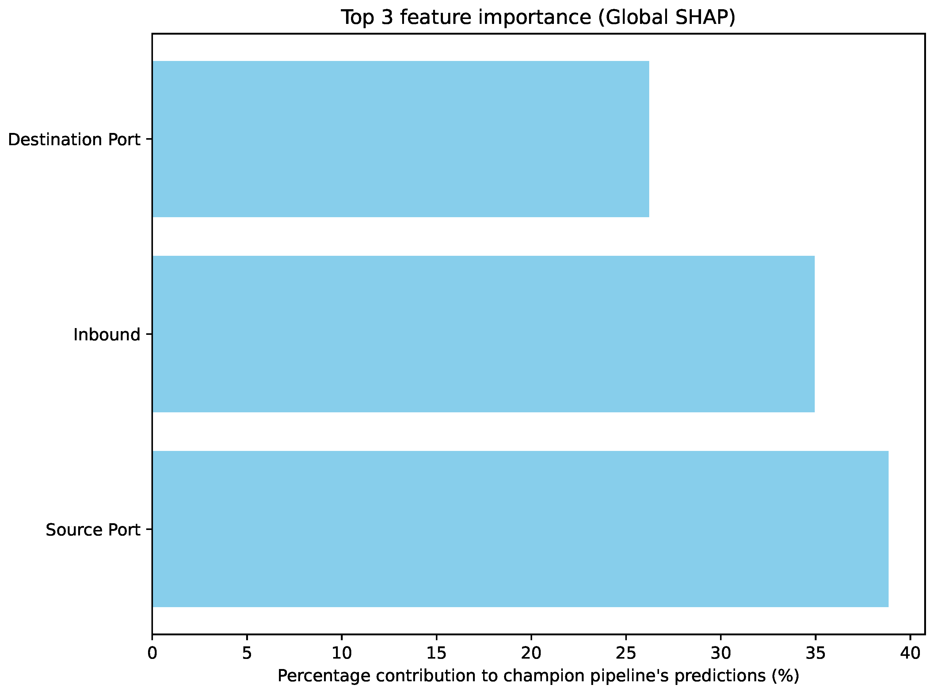
To enhance interpretability of the champion pipeline (DT_RFE_Grid_90-10), a SHapley Additive exPlanations (SHAP) analysis was conducted to quantify the contributions of each feature to the pipeline’s predictions [37]. The results of this indicate that a small subset of features consistently drive the majority of the predictive power, with top-ranked features exhibiting the largest SHAP values. In the case of the champion pipeline, only three features provide predictive information, which are: Source Port ($38.83\%$), Destination Port ($34.95\%$) and Inbound ($26.21\%$). 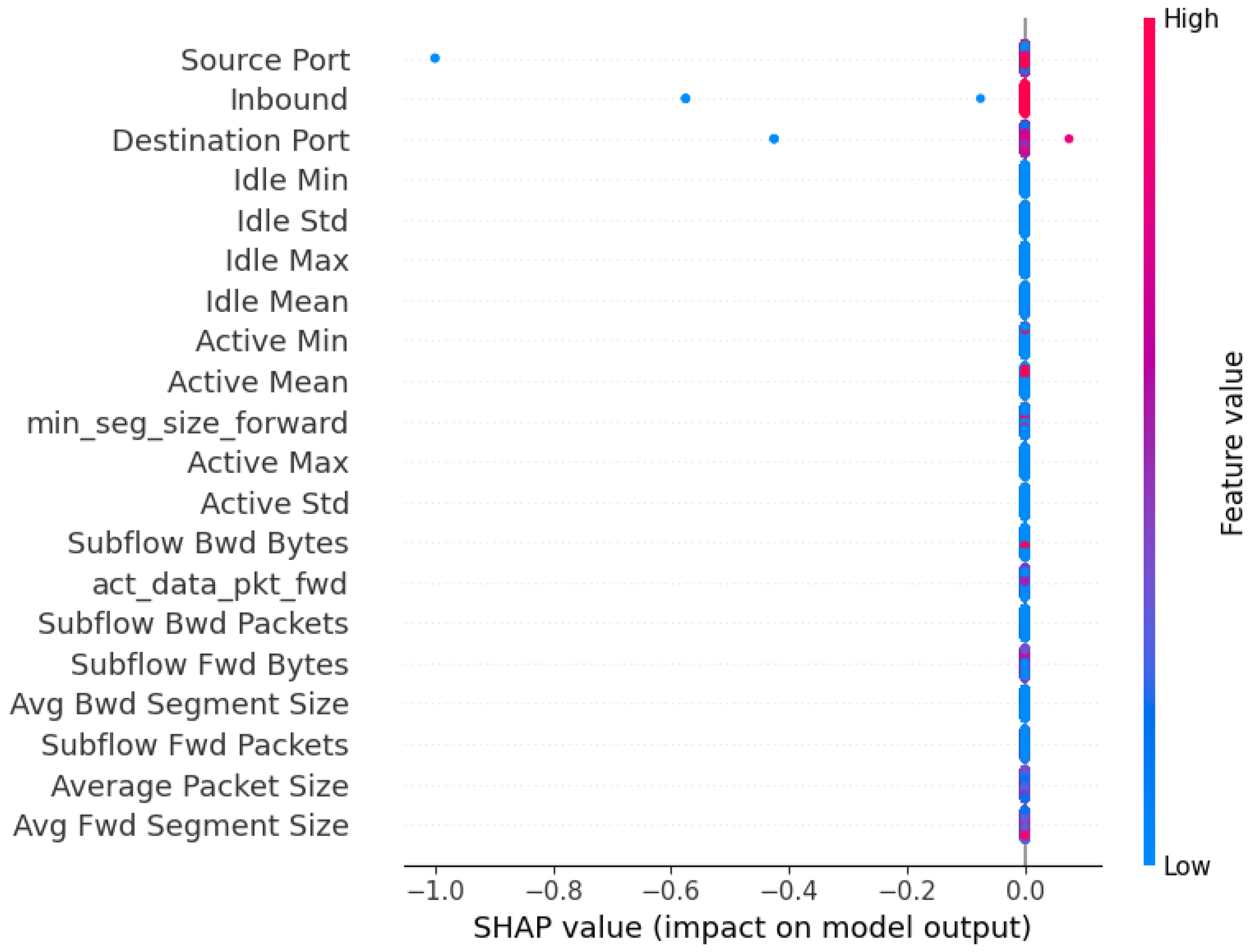These accounted for $100\%$ of the pipeline’s total predictive contribution, while the remaining features did not contribute any predictive information. The beeswarm and global feature importance plots (see Figure 3 and Figure 4) confirm that these features consistently push predictions towards or away from the positive class, highlighting their key role in the pipeline’s decision-making process. The sparsity in feature usage is a reflection of the pipeline’s inherent simplicity and interpretability; this is because DT_RFE_Grid_90-10 uses a maximum tree depth of 5 nodes, while RFE selects 20 features. The shallow tree cannot fully utilise all 20 features, which explains why only 3 features show non-zero contributions in the SHAP plots.

4.3. Generalisation and Overfitting

Generalisation is a critical requirement for reliable model deployment and assessment. As a result, the champion pipeline was evaluated on an independent dataset derived from the CIC-IDS2017 dataset [18]. A subset of approximately 25,000 samples, including both benign and DDoS-labelled traffic from the Friday afternoon attack file was extracted and adjusted to match the class distribution of the CIC-DDoS2019 subset used during pipeline development. Both datasets were obtained from the Canadian Institute for Cybersecurity using the same CICFlowMeter tool, ensuring comparable features sets, while offering differing traffic scenarios, network conditions and attack implementations. This evaluation aimed at determining whether the champion pipeline retains its high predictive performance and relatively good computational efficiency on previously unseen data, providing a robust assessment of its generalisation beyond the patterns present in the original training and testing sets.

The pre-processing steps defined in Section 3.3 were applied accordingly to this independent dataset to ensure compatibility. Similarly, the same evaluation metrics as defined in Section 3.4 were used to quantify the pipeline’s performance. To enable a fair cross-dataset comparison, the champion pipeline was constrained to feature shared by both datasets. Certain features originally selected by the RFE feature selector were not present in CIC-IDS2017, therefore, RFE was re-run restricted to the shared feature set, preserving the overall pipeline structure. Pipeline performance was evaluated across 10 random train–test splits per dataset, with the metrics reported as mean ± standard deviation to capture variability.

Furthermore, all computational metrics reported in

Table 15. Comparison of performance of the champion pipeline (DT_RFE_Grid_90-10) on the subset of the CIC-DDoS2019 dataset (CIC-DDoS2019_25K) used vs unseen dataset that is a subset of the CIC-IDS2017 dataset (CIC-IDS2017_25K) with mean and standard deviation reported for each metric.

Metric	CIC-DDoS2019_25K	CIC-IDS2017_25K
MCC	$0.8348\pm 0.1534$	$-0.1441\pm 0.3059$
F1	$0.9997\pm 0.0002$	$0.4253\pm 0.2241$
Accuracy	$0.9994\pm 0.0005$	$0.2903\pm 0.1526$
Precision	$0.9997\pm 0.0004$	$0.7988\pm 0.4210$
Recall	$0.9998\pm 0.0003$	$0.2898\pm 0.1527$
CPU Time	$0.0000\pm 0.0000$	$0.0000\pm 0.0000$
Avg. Memory Usage	$20.4\pm 1.3$	$20.0\pm 0.0$
Inference Time	$0.0008\pm 0.0000$	$0.0029\pm 0.0002$

were measured separately for training and inference, as retraining on the independent dataset would provide misleading results. Training was performed solely on the CIC-DDoS2019 subset used throughout this study. As shown in Table 15, the pipeline retained near-perfect performance, with MCC and other predictive performance metrics approaching 1.0. In contrast, on the unseen CIC-IDS2017 subset, performance can be seen to drop considerably. While precision remained moderately high, other metrics suffered significant drops, indicating the pipeline’s inability to correctly identify most DDoS samples. CPU time and memory usage remained low across inference on both datasets, with slight differences in inference time.

The results indicate that while the pipeline may perform exceptionally on the CIC-DDoS2019 subset, it exhibits very poor generalisation on unseen data. Differences in attack patterns and traffic distributions between both datasets appear to have a substantial impact on predictive performance.

4.4. Performance Trade-Offs

In evaluating models for DDoS detection and, more broadly, cyber attack detection, performance must be assessed not only from a predictive perspective but also from a computational perspective. This is because this perspective is of particular use in cases where the deployment environment is constrained by the available resources. This study reveals that while many pipelines do in fact achieve perfect or near-perfect predictive performances, trade-offs are evident when comparing them in the computational dimension.

Notably, pipelines using more complex and exhaustive hyperparameter tuning approaches like Grid Search on average only marginally increased their predictive performance while incurring a several fold increase in computational cost in metrics such as training, inference and CPU time, along with average memory usage. The fact that the results indicate diminishing returns highlights a common trade-off—that is, gaining a small increasein predictive capabilities may not be justified when the resource requirement is considered. Further, while efficiency may have appeared to play only a background role in some prior works or have been absent entirely, it is often of paramount importance in real-world deployments, alongside conventional ML metrics. For instance, a pipeline that has very high predictive performance but poor computational metrics may be deemed unsuitable for high-throughput networks. In contrast, a pipeline with marginally lower predictive capabilities but a several fold improvement in terms of memory usage and CPU time may be far more adequate.

Another less evident trade-off occurs when the maintainability and interpretability of a pipeline are an area of concern. This is because pipelines with simpler and more efficient configurations such as those using RFE and Random Search tend to be much easier to re-train, debug and maintain over time compared to those that require much more heavy computation such as Variance Threshold and Grid Search. Furthermore, tree-based models, shown in this study to be well-suited for the DDoS detection task, offer greater interpretability advantages compared to other supervised classifiers. Their tree structure enables security analysts to visualise decision paths and understand which features drive predictions. This transparency supports bias detection, maintainability and informed decision making based on the model’s structure and outputs.

All things considered, the selection of a pipeline and its respective components for production and use often involves a much more comprehensive and context-tailored approach that goes beyond using the best pipeline in terms of conventional ML metrics. It often requires an adequate balance between predictive and computational performance along with other trade-offs to be considered, all of which shape the decision made in relation to the pipeline design process. As demonstrated in this study, the most performant pipelines are not always the most computationally efficient and vice versa; this underscores the importance and necessity of evaluating all these trade-offs using a holistic and nuanced evaluatory framework.

5. Conclusions

In this study, 210 unique ML pipelines comprising five supervised classifiers, three feature selectors, two hyperparameter tuners and seven train–test splits were evaluated against conventional and computational metrics. The results show that tree-based classifiers tend to outperform the other supervised ML classifiers that were investigated, achieving higher MCC while also demonstrating superior training and inference times, which aligns with prior works. Among the explored feature selection methods, SelectKBest emerged as the feature selector with highest average MCC; however, in comparison, RFE showcased lower computational costs with slightly worse MCC. Random Search was identified to have superior computational efficiency when compared to Grid Search in terms of training time and CPU time, with slight predictive performance loss. Overall, although RF-based pipelines achieved slightly higher MCC on average than DT-based pipelines, the difference was marginal, and thus, as DT-based pipelines have much lower training, inference and CPU times along with lower memory usage on average, they represent the best compromise in terms of balancing predictive performance and computational performance.

These findings seek to provide actionable guidance for researchers and industry professionals who develop ML pipelines for DDoS detection in resource-conscious environments. The results demonstrate that tree-based methods are able to deliver competitive predictive performance at much lower computational cost, providing an attractive alternative to more resource-intensive approaches. More broadly, this study highlights the value and necessity of evaluating ML pipelines across multiple dimensions, with computational metrics revealing trade-offs that have remained unclear or underreported in prior works that relied solely on conventional metrics.

However, this study is also not without its limitations, which are discussed below:

• Limited sample size: Due to computational constraints, this study utilised a representative subset of approximately 25,000 samples from the full CIC-DDoS2019 dataset, which contains over 70 million records. Although this subset was selected to closely reflect the original dataset’s distribution, it may not have fully captured the variability and nuances present in the complete dataset. As a result, the reported findings should be interpreted with this limitation in mind. Future work should explorer larger samples, if feasible, to further validate the generalisability of the results.
• Memory profiling methodology: Memory usage was monitored using a threaded sampling approach with periodic intervals (≈100 ms). While this provides a general overview of a pipeline’s memory consumption, it may not capture short-lived peak usage spikes. As a result, the reported memory metric may underestimate the true average memory usage. Future work should seek to employ more precise profiling tools or methods to capture more fine-grained memory consumption behaviour and more accurately characterise a given pipeline’s memory usage.
• Pipeline exploration scope: Despite the comprehensive nature of this study, it remains limited by the range of supervised classifiers, feature selectors, hyperparameter tuning methods and parameter grids explored. The lack of exploration of alternative paradigms, such as unsupervised learning, further restricts the generalisability of the findings. Additionally, while computational metrics such as memory usage and CPU time served as valid comparators across the explored pipelines, the results obtained for them may not fully reflect the true performance of said pipelines in different deployment environments. Future work should extend this multi-dimensional evaluation framework to include a broader set of classifiers, more advanced hyperparameter tuning techniques, more extensive parameter grids and diverse datasets to better assess its robustness and applicability.
• Cross-dataset feature restriction: Evaluation of the champion pipeline’s generalisability was limited to the features shared between both the CIC-DDoS2019 and CIC-IDS2017 datasets to ensure comparability. While this approach helped in some aspects, it may have constrained the pipeline’s performance by excluding informative features such as Source Port that were unique to either dataset.

In conclusion, this study aimed to lay a foundation for the idea of multi-dimensional evaluation of ML pipelines, not just for DDoS detection but in other research avenues too, exploring both predictive and computational performance. This is because it hopes to aid in the development of more efficient and scalable ML-based solutions that can be directly applied from future studies to future industry solutions with minimal difficulty.