Cost Parameters-Based Comprehensive Analysis of a New Cost Function Construction for Coxian-k Queueing System Characterized by Customer Service Speed Variability

Abstract

We investigate cost optimization in an $M/{\mathrm{Cox}}_k/1$ queueing system with phase-dependent service speeds. A unified parametric framework is introduced to model both homogeneous and heterogeneous service regimes, and closed-form expressions for steady-state performance measures are derived. These results are used to construct an expected total cost function explicitly parameterized by the traffic intensity. We prove that the cost function is strictly convex on the stability region, ensuring the existence and uniqueness of the optimal traffic intensity. For the Coxian-2 case, analytical and numerical sweep analyses are conducted with respect to waiting and service-capacity cost parameters. Polynomial response surfaces and nonparametric statistical tests are employed to validate the robustness of the results. The analysis shows that balanced service speeds across phases consistently yield lower optimal traffic intensity levels and reduced expected total costs, whereas heterogeneous service speeds increase congestion and cost sweep. These findings provide practical guidance for the economic design and control of multi-phase service systems.

1. Introduction

Queueing systems with complex service mechanisms, particularly those involving multi-phase structures, have become essential tools for modeling and analyzing service-based operations in various domains, such as telecommunications, healthcare, and manufacturing. Among these, systems with Coxian service times stand out due to the analytical flexibility of the Coxian distribution, which generalizes both Erlang and hypoexponential distributions. Its ability to represent a wide range of service behaviors through phase-dependent parameters makes it well suited for realistic service time modeling. In recent years, increasing attention has been devoted to integrating performance measures with cost-based decision making in such queueing models. However, comprehensive cost function formulations for systems with Coxian service times remain relatively scarce in the literature. This paper addresses this gap by constructing and analyzing a cost function for the $M/Co{x}_k(p_1,\dots ,p_{k-1};{\mu }_1,\dots ,{\mu }_k)/1$ queueing system, incorporating the impact of both constant and variable customer service speeds across phases. Our approach builds upon previous foundational studies and aims to optimize system performance under operational efficiency constraints.

In addition to their analytical tractability, Coxian distributions possess a phase-type structure that enables an efficient modeling of heterogeneous service environments, in which customer progression depends not only on stochastic service durations but also on control-based system configurations. This flexibility is particularly valuable in operational contexts that require differentiated treatment across stages, such as triage in healthcare systems or multi-step manufacturing workflows, where service acceleration or deceleration in certain phases directly affects throughput, congestion, and costs. Despite this practical relevance, the existing literature predominantly focuses on performance metrics such as queue length, sojourn time, or server traffic intensity, while cost-aware formulations are often restricted to simpler service models. Integrating cost components, such as waiting costs and the amortization of service infrastructure, into multi-phase systems presents a significant analytical challenge due to the nonlinear interplay among service time distributions, customer behavior, and operational decisions. Only limited contributions attempt such integration, and these typically address special cases such as Erlang or hypoexponential distributions with equal phase durations or simplified cost structures.

This paper seeks to bridge this gap by proposing a general and analytically tractable cost function tailored to the $M/Co{x}_k(p_1,\dots ,p_{k-1};{\mu }_1,\dots ,{\mu }_k)/1$ system. We explicitly incorporate customer service speed variability across phases, which generalizes both constant-speed and phase-varying service models. This approach enables a unified analysis of systems with uniform or heterogeneous service speeds and provides a meaningful cost–performance trade-off.

The remainder of the paper is organized as follows. Section 2 reviews existing literature on Coxian phase-type distributions, queueing models with structured service times, and prior approaches to cost function analysis in single-server systems. In Section 3, we review the structure of Coxian distributions and introduce the queueing system model. Section 4 develops an analytical framework for performance measures based on service speed. In Section 5, we propose and examine a cost function tied to customer service speed and derive an optimal traffic intensity. Section 6 presents sweep and statistical analyses based on changes in cost parameters as well as additional difference-based evaluation using the Wilcoxon signed-rank test. Section 7 concludes the paper with a summary of the findings and provides some practical insights. Finally, Section 8 provides the limitations of the presented work and directions for further research.

2. Related Work

Coxian phase-type (PH) distributions and their integration into queueing models have been extensively studied due to their analytical flexibility and ability to approximate a broad class of service time distributions. Among the foundational contributions, He and Zhang [1] developed a rigorous framework for approximating general matrix-exponential distributions using ordered Coxian structures. Their results provide strong theoretical justification for employing Coxian forms to achieve computational tractability in systems where service processes exhibit multi-stage or phase-like behavior. Parameter estimation and numerical aspects of PH distributions have also been investigated in detail, for example in the doctoral work of Esparza [2].

2.1. Structural Properties and Service Parameter Optimization

Several studies have examined how the internal structure of Coxian models influences system performance. In particular, Sağlam et al. [3] analyzed the effect of ordering service speeds in a three-phase Coxian queueing system and demonstrated that optimal sequencing can significantly reduce the average system delay. Their findings highlight the importance of parameter design in multi-phase service models and directly support our modeling approach, where service speeds and transition probabilities are treated as controllable design variables linked to system efficiency and cost.

2.2. Matrix-Analytic Methods and PH-Based Queueing Models

The matrix-analytic framework for PH distributions was pioneered by Marcel F. Neuts and has become central to modern queueing theory. The monograph Neuts [4] and the review article Alfa [5] describe matrix-geometric and matrix-analytic techniques for analyzing $M/G/1$-type systems with PH service times. These methods enable a closed-form or semi-closed-form analysis of complex models that are otherwise intractable using classical approaches. A comprehensive overview of matrix-analytic stochastic modeling is provided in Neuts [6], where the role of matrix exponentials and phase-based subgenerator structures is emphasized.

Subsequent work has extended these techniques to more elaborate settings. For example, Chakravarthy et al. [7] considered queueing systems with Markovian arrivals, PH service times, server breakdowns, and repairs, demonstrating the robustness of PH-based modeling in failure-prone environments. Computational approaches for related models were discussed in Hochrainer et al. [8], which proposed an algorithm for computing steady-state probabilities in $M/E_r/c/K$ systems. Since Erlang distributions form a subclass of PH distributions, their methodology naturally extends to Coxian representations and aligns with our matrix-based formulation for performance and cost analysis.

2.3. Queueing Models with Priorities, Parallel Servers, and Numerical Aspects

PH distributions have also been employed in multi-server and priority settings. In Al Hanbali et al. [9], approximations for the waiting-time distribution in $M/PH/c$ priority queues were derived, providing insight into systems where exact analysis is computationally prohibitive. Related numerical techniques for the structured matrices arising in PH-based models were investigated in Jia et al. [10]. Although this paper focuses on a single-server configuration, it complements this line of research by providing new analytical expressions and structural insights in support of cost-optimization objectives.

2.4. Applications of Coxian and PH Models

Over the last two decades, numerous applied studies have used Coxian and PH distributions to model realistic service systems. Examples include processor-sharing queues with impatient customers [11], $M/G/1$ queues with working vacations and interruptions [12], and closed queueing networks for fleet sizing in logistics systems [13]. In the healthcare domain, Jen et al. [14] proposed a Coxian hurdle model for population-based cancer screening, while Thompson et al. [15] applied queueing theory to evaluate the effectiveness of triage algorithms in reducing patient waiting times. Flow-line systems with Cox-2 service times and limited buffers were analyzed in Helber [16], and more recently, Anggraito et al. [17] studied a multi-server priority queue with two job classes and Cox-2 distributed service times. Extensions to time-dependent environments were considered in Andersen [18]. On the theoretical side, Protter and Riveros Valdevenito [19] investigated Markov jump times via Cox constructions, while Rudec and Manger [20] developed fast approximation methods for the k-server problem. A new congestion measure for emergency departments was proposed in Wartelle et al. [21]. Together, these works demonstrate the broad applicability of Coxian and PH modeling in both theoretical and applied settings.

More recent contributions further highlight the flexibility of PH and Coxian models in capturing structural heterogeneity and complex service mechanisms. In Sinu Lal et al. [22], a multi-type queueing–inventory system for spectrum selection and allocation was developed using phase-type service representations to model differentiated customer demands and resource consumption. Algorithmic aspects of PH-based queueing models in random environments were addressed by Dudin et al. [23], who studied systems with a varying number of servers and arrival processes modulated by an external stochastic environment.

Phase-type distributions have also been successfully employed beyond classical service systems. A PH-based stochastic model for random telegraph noise in resistive memory devices was proposed in Ruiz-Castro et al. [24], while García-Mora et al. [25] introduced a new PH distribution for the sum of concatenated Markov processes with applications to survival analysis in bladder cancer. In the context of actuarial science, Asmussen et al. [26] demonstrated how PH models can be used for the fitting and valuation of equity-linked life insurance products.

Methodological advances combining PH models with modern data-driven techniques were reported in Vishnevsky et al. [27], where a fork-join queue with MAP arrivals and PH service times was analyzed using machine learning methods. Furthermore, Chakravarthy [28] investigated queueing systems with MAP input and heterogeneous phase-type group services, providing insights into performance evaluation under complex service structures. Although outside the queueing domain, the study in Machado et al. [29] illustrates how multi-phase stochastic modeling ideas also arise in the control and validation of three-phase photovoltaic systems. These studies reinforce the role of Coxian and PH distributions as a powerful and unifying modeling framework for multi-stage service processes across a wide spectrum of application areas.

2.5. Cost Modeling in Multi-Phase Queueing Systems

Despite the extensive literature on PH-based performance analysis, cost function modeling for Coxian queues remains comparatively limited. A notable recent contribution is Immaculate and Rajendran [30], which analyzed the economic performance of a two-phase Coxian system with encouraged arrivals and customer balking. Their model incorporates waiting and service-related costs and illustrates how system configurations affect both performance and operating expenses.

Several related studies have addressed cost modeling under simpler service assumptions. In Mirchevski and Bakeva [31], a cost function was constructed and analyzed for an $M/E_k/1$ queue, and its sweep with respect to the traffic intensity $\rho$ and the number of phases k was derived. An extension to hypoexponential-2 service times was presented in Mirchevski and Bakeva [32], including computational illustrations and parametric studies. These works were further expanded in Mirchevski et al. [33] and Mirchevski et al. [34], where broader classes of multi-phase systems and new optimization formulations were considered.

2.6. Positioning of the Present Work

In summary, while existing studies have separately investigated Coxian modeling, matrix-analytic methods, and cost optimization in queueing systems, their joint integration remains limited. This paper contributes to the literature by proposing a general cost function formulation for Coxian-k service systems with phase-dependent service speeds. The proposed framework generalizes earlier two-phase and constant-speed models, yields tractable expressions for key performance measures, and leads to a closed-form polynomial equation for determining optimal operating points under operational efficiency constraints. The main contribution of this paper lies in the construction of a cost function that explicitly incorporates two essential components. The first is a waiting cost rate, which is defined as the product of the unit waiting cost and the expected number of customers in the system rather than the expected waiting time, which is more commonly adopted in the literature. The second component is an amortization cost rate that reflects the multi-phase structure of the service process. Instead of assuming a single amortization cost associated with a single server, we introduce phase-dependent amortization costs, resulting in k distinct cost terms corresponding to the k service phases. This formulation captures the heterogeneity of service speeds across phases, since each phase operates with a different service speed and therefore incurs a different operational cost.

3. Coxian Model and Coxian Distribution

Consider a finite continuous-time Markov process $\left\{\mathit{X}\right(t):t\ge 0\}$ with discrete state space $\{1,\dots ,k,k+1\}$, where $k\in \mathbb{N}$. States 1 through k are transient, whereas state $k+1$ is absorbing. Let $s_i=P(\mathit{X}\left(0\right)=i)$, $i=1,\dots ,k$, denote the probability that the process starts in transient state i. In the Coxian model, the process starts in the first phase; hence, the initial distribution is $\mathbf{s}=(1,0,\dots ,0)$, where $\mathbf{s}$ is a k-dimensional row vector. Starting from state i ($i=1,\dots ,k$), the process may jump directly to the absorbing state $k+1$ with a certain probability. Let $\mathbf{S}$ denote the $k\times k$ subgenerator matrix of transition rates among the transient states. In probability theory, the pair $(\mathbf{s},\mathbf{S})$ is called a representation of the Coxian phase-type distribution.

It is well known that the Coxian model can be used to describe queueing systems in which the customer service time consists of k phases and follows a Coxian-k distribution. In the Coxian model, the service requires at most k phases, and the service time in each phase i is exponentially distributed with parameter ${\mu }_i>0$, $i=1,\dots ,k$. After completing phase $j<k$, the customer proceeds to the next phase with probability $p_j$ or completes the service and leaves the system with probability $q_j=1-p_j$, $j=1,\dots ,k-1$. The parameter ${\mu }_i$, $i=1,\dots ,k$, is also referred to as the total rate of leaving phase i. Accordingly, the subgenerator matrix $\mathbf{S}$ for the Coxian model has the form

$$\mathbf{S}={\left[\begin{array}{ccccccc}-{\mu }_1& p_1{\mu }_1& 0& \cdots & 0& 0& 0\\ 0& -{\mu }_2& p_2{\mu }_2& \cdots & 0& 0& 0\\ 0& 0& -{\mu }_3& \cdots & 0& 0& 0\\ ⋮& ⋮& ⋮& \ddots & ⋮& ⋮& ⋮\\ 0& 0& 0& \cdots & -{\mu }_{k-2}& p_{k-2}{\mu }_{k-2}& 0\\ 0& 0& 0& \cdots & 0& -{\mu }_{k-1}& p_{k-1}{\mu }_{k-1}\\ 0& 0& 0& \cdots & 0& 0& -{\mu }_k\end{array}\right]}_{k\times k}.$$

(1)

In general, the Coxian-k distribution is a continuous distribution on $[0,+\infty )$ with parameters ${\mu }_i>0$, $i=1,\dots ,k$, and probabilities $0\le p_j\le 1$, $j=1,\dots ,k-1$. According to the above description, the Coxian-k distribution generalizes both Erlang and hypoexponential distributions. Specifically, if $p_j=1$ for $j=1,\dots ,k-1$ and ${\mu }_i=\mu$ for $i=1,\dots ,k$, then it reduces to the Erlang-k distribution with common parameter $\mu$. If $p_j=1$ only for $j=i,\dots ,k-1$, then it reduces to a hypoexponential-k distribution with distinct parameters ${\mu }_i$, $i=1,\dots ,k$.

Let X be a random variable representing the total customer service time over all k phases, and assume that X follows the Coxian-k distribution with parameters ${\mu }_i$, $i=1,\dots ,k$, and probabilities $p_j$, $j=1,\dots ,k-1$, i.e., $X\sim Co{x}_k(p_1,\dots ,p_{k-1};{\mu }_1,\dots ,{\mu }_k)$. Then, the probability density function of X can be written in the following matrix form:

$$f_X\left(t\right)=\mathbf{s}·\exp \left(\mathbf{S}t\right)·\mathbf{r},$$

(2)

where $\mathbf{S}$ is the $k\times k$ subgenerator matrix among the transient states, $\mathbf{s}=(1,0,\dots ,0)$ is the k-dimensional input row vector, and $\mathbf{r}=-\mathbf{S}·\mathbf{1}$ is the k-dimensional output column vector (absorption rate vector), with $\mathbf{1}$ denoting the k-dimensional column vector of ones, and $t\ge 0$. The expression $\exp \left(\mathbf{S}t\right)$ denotes the matrix exponential of $\mathbf{S}t$; it can be computed via the power series $\exp \left(\mathbf{S}t\right)={\sum }_{k=0}^{+\infty }{\displaystyle \frac{t^k{\mathbf{S}}^k}{k!}}$. It is important to note that there is no closed-form expression for (2). Nevertheless, using matrix-analytic methods and keeping (2) in its matrix form, one can compute the moments of X of any order for a k-phase Coxian model. The following lemma is a standard result and will be useful in the subsequent analysis.

Lemma 1.

The states $1,\dots ,k$ of the Coxian model are transient if and only if the subgenerator matrix $\mathbf{S}$ is nonsingular.

Proof. 

See Lemma 2.2.1, p. 45 in Neuts [4], which is stated for general PH distributions (including the Coxian distribution). □

The matrix $\mathbf{S}$ in (1) is an upper bidiagonal subgenerator matrix of a Coxian-k model. Its spectrum consists of its diagonal entries,

$$\sigma \left(\mathbf{S}\right)=\{-{\mu }_1,-{\mu }_2,\dots ,-{\mu }_k\},$$

where ${\mu }_i>0$ for all $i=1,\dots ,k$. Hence, all eigenvalues of $\mathbf{S}$ are strictly negative real numbers. Since $0\notin \sigma \left(\mathbf{S}\right)$, the matrix $\mathbf{S}$ is nonsingular, and therefore its inverse ${\mathbf{S}}^{-1}$ exists and is unique. This confirms that the subgenerator matrix $\mathbf{S}$ is invertible.

4. Description of the $\mathit{M}/{\mathit{Cox}}_{\mathit{k}}({\mathit{p}}_{\mathbf{1}},\dots ,{\mathit{p}}_{\mathit{k}-\mathbf{1}};{\mathit{\mu }}_{\mathit{1}},\dots ,{\mathit{\mu }}_{\mathit{k}})/\mathbf{1}$ Queueing System Characterized by Customer Service Speed Variability

In this section, we consider a queueing system of type $M/Co{x}_k(p_1,\dots p_{k-1};{\mu }_1,\dots ,{\mu }_k)/1$. In addition to the general preliminaries and standard modeling assumptions, we introduce an approach for model construction based on customer service speed variability across phases and derive the complete analytical results associated with this framework.

4.1. Preliminaries

We first provide a brief description of the main components of the considered queueing system, which is characterized by a Poisson arrival process and Coxian-k distributed service times. Throughout the paper, we use the short notation $M/Co{x}_k(p_1,\dots p_{k-1};{\mu }_1,\dots ,{\mu }_k)/1$, which indicates the following:

• The input stream follows a Poisson process with parameter $\lambda >0$;
• The service time is distributed according to $Co{x}_k(p_1,\dots p_{k-1};{\mu }_1,\dots ,{\mu }_k)$. Specifically, customer service consists of k exponentially distributed phases with parameters ${\mu }_i>0$, $i=1,\dots ,k$, such that after completing service in phase j, the customer either proceeds to the next phase with probability $p_j$, $j=1\dots ,k-1$ or leaves the system with probability $q_j=1-p_j$, $j=1,\dots ,k-1$;
• Service is provided by a single server.

A detailed description of the Coxian service mechanism is given in Section 3.

4.2. General Assumptions

In this subsection, we summarize the general assumptions underlying the proposed $M/Co{x}_k(p_1,\dots p_{k-1};{\mu }_1,\dots ,{\mu }_k)/1$ queueing system.

• Customers arrive according to a Poisson process with rate $\lambda$;
• Service times follow a Coxian-k phase-type distribution characterized by phase transition probabilities $(p_1,\dots ,p_{k-1})$ and phase-dependent service speeds $({\mu }_1,\dots ,{\mu }_k)$;
• Customers are served according to the FIFO (first-in, first-out) discipline;
• Infinite buffer (waiting room);
• Service of the next customer begins immediately after the completion of service of the previous customer;
• Arrival and service processes are mutually independent, and successive service times are independent and identically distributed;
• The traffic intensity is defined as

  $$\rho =\lambda \mathbb{E}X,$$

  and the system operates in steady state if $0<\rho <1$. A detailed matrix and symbolic representation of $\rho$ for the considered model is provided in Section 4.3 and Section 5. In further analyses, $\rho$ is a decision variable.

We can see that under certain special conditions, $\rho$ can be reduced to a simpler form, which is suitable for some special cases of systems. We list the most important special cases below.

• The $M/{\mathrm{Hypo}}_k/1$ queueing system with k phases and hypoexponential-k service time across the phases. The traffic intensity is

  $$\rho ={\displaystyle \frac{\lambda {\sum }_{j=1}^k{\prod }_{i=1,i\ne j}^k{\mu }_i}{{\prod }_{i=1}^k{\mu }_i}},$$

  obtained for $p_j=1$, $j=1,\dots ,k-1$ in the current Coxian queueing system.
• The $M/{\mathrm{Erlang}}_k/1$ queueing system with k phases and Erlang-k service time across the phases. The traffic intensity is

  $$\rho ={\displaystyle \frac{\lambda k}{\mu }},$$

  obtained for ${\mu }_i=\mu$, $i=1,\dots ,k$ and $p_j=1$, $j=1,\dots ,k-1$ in the current Coxian queueing system.
• The $M/M/1$ queueing system with one phase and exponential service time. The traffic intensity is

  $$\rho ={\displaystyle \frac{\lambda }{\mu }},$$

  obtained for ${\mu }_i=\mu$, $i=1,\dots ,k$, $p_j=1$, $j=1,\dots ,k-1$ and $k=1$ in the current Coxian queueing system.

4.3. An Approach Characterized by Customer Service Speed Variability

We now introduce an approach that unifies two modeling scenarios: (i) phase-dependent service speeds and (ii) identical service speeds across all phases. Both cases can be expressed through a single parametric relation. Specifically, we assume that the service speeds satisfy

$${\mu }_i={\mu }_1{\alpha }^{i-1},i=1,\dots ,k.$$

For the first scenario, we allow the service speed to systematically increase or decrease across phases, corresponding to $\alpha >0$ and $\alpha \ne 1$. If $0<\alpha <1$, successive phases become slower, meaning that each phase serves customers at a lower average rate than the previous one. Conversely, if $\alpha >1$, the service speed increases across phases.

For the second scenario, $\alpha =1$, implying ${\mu }_1=\cdots ={\mu }_k=\mu$. In this case, the model reduces to a system with identical service speeds in all phases. Clearly, this scenario constitutes a special case of the general formulation.

Why a geometric progression for phase speeds?

To keep the multi-phase model parsimonious while still allowing heterogeneous phase speeds, we parameterize the service speeds by a single phase speed $\alpha$ via ${\mu }_i={\mu }_1{\alpha }^{i-1}$. From an applied perspective, many service processes are inherently sequential and stage-dependent (e.g., clinical deterioration pathways, diagnostic/treatment stages, and multi-step processing pipelines), where transition or completion rates naturally vary across stages and can be interpreted as “rates of flow” through ordered phases according to Donnelly et al. [35]. In such settings, a geometric trend provides a compact and interpretable first-order approximation of systematic stage-to-stage speed changes while avoiding the over-parameterization typically associated with fully unconstrained phase-type specifications.

Under this parameterization, the subgenerator matrix $\mathbf{S}$ takes the form

$$\mathbf{S}={\left[\begin{array}{ccccccc}-{\mu }_1& p_1{\mu }_1& 0& \cdots & 0& 0& 0\\ 0& -{\mu }_1\alpha & p_2{\mu }_1\alpha & \cdots & 0& 0& 0\\ 0& 0& -{\mu }_1{\alpha }^2& \cdots & 0& 0& 0\\ ⋮& ⋮& ⋮& \ddots & ⋮& ⋮& ⋮\\ 0& 0& 0& \cdots & -{\mu }_1{\alpha }^{k-3}& p_{k-2}{\mu }_1{\alpha }^{k-3}& 0\\ 0& 0& 0& \cdots & 0& -{\mu }_1{\alpha }^{k-2}& p_{k-1}{\mu }_1{\alpha }^{k-2}\\ 0& 0& 0& \cdots & 0& 0& -{\mu }_1{\alpha }^{k-1}\end{array}\right]}_{k\times k},$$

(3)

for $\alpha >0$ and $\alpha \ne 1$, and

$$\mathbf{S}={\left[\begin{array}{ccccccc}-\mu & p_1\mu & 0& \cdots & 0& 0& 0\\ 0& -\mu & p_2\mu & \cdots & 0& 0& 0\\ 0& 0& -\mu & \cdots & 0& 0& 0\\ ⋮& ⋮& ⋮& \ddots & ⋮& ⋮& ⋮\\ 0& 0& 0& \cdots & -\mu & p_{k-2}\mu & 0\\ 0& 0& 0& \cdots & 0& -\mu & p_{k-1}\mu \\ 0& 0& 0& \cdots & 0& 0& -\mu \end{array}\right]}_{k\times k},$$

(4)

for $\alpha =1$.

To establish the main performance results of the model, we first state the following lemma.

Lemma 2.

Let $X\sim Co{x}_k(p_1,\dots ,p_{k-1};{\mu }_1,\dots ,{\mu }_k)$, where ${\mu }_i={\mu }_1{\alpha }^{i-1}$, $i=1,\dots ,k$, for $\alpha >0$. Then, the n-th moment of X is given by

$$\mathbb{E}{X}^n={(-1)}^{n}n!\mathit{s}{\mathit{S}}^{-n}\mathit{1},$$

where $n\in \mathbb{N}$, $\mathit{S}$ is defined by (3) or (4), $\mathit{s}=(1,0,\dots ,0)$ is the k-dimensional input row vector, and $\mathit{1}$ is the k-dimensional column vector of ones.

Proof. 

The result follows by induction on n, using the matrix exponential integral

$${\int }_0^{+\infty }t{e}^{\mathbf{S}t}dt={\mathbf{S}}^{-2}$$

together with Lemma 1. See Theorem 2.7, pp. 10–12 in Esparza [2], for the general case with arbitrary ${\mu }_i>0$, $i=1,\dots ,k$. □

We further introduce two auxiliary random variables: N, denoting the number of customers in the system at an arbitrary time instant, and W, denoting the waiting time of a customer in the queue. Before deriving the main analytical results, we briefly outline the approach used to obtain the steady-state performance measures of the proposed system. The Coxian-k service-time distribution is represented in matrix form, which enables an explicit computation of its first two moments using matrix-analytic techniques. These moments are then substituted into classical results for the $M/G/1$ queue—in particular, the Pollaczek–Khinchine formula for the mean system size and waiting time. This procedure allows all performance measures to be expressed in closed form as functions of the traffic intensity $\rho$ and the service-phase speeds. The resulting expressions form the analytical foundation for the construction and optimization of the cost function in the subsequent sections.

Theorem 1.

For the proposed $M/Co{x}_k(p_1,\dots p_{k-1};{\mu }_1,\dots ,{\mu }_k)/1$ queueing system operating in steady state and characterized by customer service speed variability ($\alpha >0$), the traffic intensity ρ, the expected waiting time $\mathbb{E}W$, and the expected number of customers in the system $\mathbb{E}N$ are given in matrix form by

$$\rho =-\lambda \mathit{s}{\mathit{S}}^{-1}\mathit{1},\mathbb{E}W={\displaystyle \frac{\lambda \mathit{s}{\mathit{S}}^{-2}\mathit{1}}{1-\rho }},\mathbb{E}N=\rho +{\displaystyle \frac{{\lambda }^2\mathit{s}{\mathit{S}}^{-2}\mathit{1}}{1-\rho }},$$

where $\mathit{S}$ is defined by (3) or (4), $\mathit{s}=(1,0,\dots ,0)$, and $\mathit{1}$ is the k-dimensional column vector of ones.

Proof. 

By Lemma 2, the traffic intensity satisfies

$$\rho =\lambda \mathbb{E}X=-\lambda \mathbf{s}{\mathbf{S}}^{-1}\mathbf{1}.$$

To compute the expected waiting time, we apply the classical Pollaczek–Khinchin formula,

$$\mathbb{E}W={\displaystyle \frac{\lambda \mathbb{E}{X}^2}{2(1-\rho )}}.$$

Using Lemma 2 again yields

$$\mathbb{E}W={\displaystyle \frac{\lambda \mathbf{s}{\mathbf{S}}^{-2}\mathbf{1}}{1-\rho }}.$$

Let T denote the sojourn time of a customer in the system (waiting time plus total service time). By linearity of expectation,

$$\mathbb{E}T=\mathbb{E}W+\mathbb{E}X.$$

Finally, applying Little’s law gives

$$\mathbb{E}N=\lambda \mathbb{E}T=\rho +{\displaystyle \frac{{\lambda }^2\mathbf{s}{\mathbf{S}}^{-2}\mathbf{1}}{1-\rho }}.$$

□

5. Construction and Analysis of a Cost Function for $\mathit{M}/{\mathit{Cox}}_{\mathit{k}}({\mathit{p}}_{\mathbf{1}},\dots ,{\mathit{p}}_{\mathit{k}-\mathbf{1}};{\mathit{\mu }}_{\mathbf{1}},\dots ,{\mathit{\mu }}_{\mathit{k}})/\mathbf{1}$ Queueing System Characterized by Customer Service Speed Variability

This section presents results on the construction and analysis of a cost function for the $M/Co{x}_k(p_1,\dots p_{k-1};{\mu }_1,\dots ,{\mu }_k)/1$ queueing system, expressed in terms of the traffic intensity, under the assumption that the service speeds ${\mu }_i$, $i=1,\dots ,k$, are unknown. In this way, a strictly convex function on the interval $(0,1)$ can be constructed, the optimization of which can be easily carried out through derivatives. On the other hand, after finding the optimal traffic intensity ${\rho }^{*}$, due to the relation between the service speeds ${\mu }_i$ and the traffic intensity $\rho$ given by $\rho =-\lambda \mathbf{s}{\mathbf{S}}^{-1}\mathbf{1}$ in Theorem 1, the corresponding optimal speeds ${\mu }_i^{*}$, $i=1,\dots ,k$ can be found. So, controlling the optimal service speeds across the phases is determined by the optimal traffic intensity. It is important to note that if the cost function is treated as a function of multiple variables, for example, $\lambda >0$, ${\mu }_1,\dots ,{\mu }_k>0$ under a single condition $0<\rho <1$, then the function is not convex and can be optimized by some metaheuristic algorithms for global optimization. Precisely because of the idea of representing the function through $\rho$, it is necessary to represent all service speeds ${\mu }_i$, $i=1,\dots ,k$ through one service speed in order to be covered by $\rho$ and their optimal choice to depend initially on the optimal traffic intensity—hence the idea of introducing a factor $\alpha$ based on a geometric progression to determine the speeds through the phases. Of course, this is one way to express all ${\mu }_i$, $i=1,\dots ,k$ through the first service speed, but it is not the only one. In practice, if we are talking about production where the mechanism of operation of the phases can be controlled, the rule of how the speeds change between the phases can be determined, and accordingly the speeds can be approximately expressed through one of them. The proposed formulation captures the operational behavior of the system and enables both an analytical and numerical investigation of how $\rho$ influences performance and cost.

The construction of the cost function is based on two components: (i) the expected waiting cost per customer per unit time, denoted by $C_w$, and (ii) the expected system cost associated with server amortization (depreciation) across phases per customer per unit time, which is denoted by $C_s$. Accordingly, we define the expected total cost by

$$\mathsf{\Phi }=C_w+C_s,$$

where $\mathsf{\Phi }$ denotes the expected total system cost. Using the performance measures derived in Theorem 1, we adopt the following interpretation of $C_w$ and $C_s$:

• $C_w$ is given by the product of the waiting cost rate $c_w>0$ (per customer per unit time) and the expected number of customers in the system, $\mathbb{E}N$, i.e.,

  $$C_w=c_w\mathbb{E}N=c_w\left(\rho +{\displaystyle \frac{{\lambda }^2\mathbf{s}{\mathbf{S}}^{-2}\mathbf{1}}{1-\rho }}\right);$$
• For $\alpha >0$ and $\alpha \ne 1$, $C_s$ is a linear combination of the phase-wise amortization costs $c_i>0$, $i=1,\dots ,k$, and the corresponding service speeds ${\mu }_i>0$, $i=1,\dots ,k$, i.e.,

  $$C_s=c_i{\mu }_i;$$
• For $\alpha =1$, we have $c_i=c>0$ and ${\mu }_i=\mu >0$, $i=1,\dots ,k$, so that $C_s$ becomes a linear combination of the common amortization cost c and the common service speed $\mu$, i.e.,

  $$C_s=kc\mu .$$

In practice, the relationship between service capacity and operating or capital cost may be nonlinear due to technological constraints, economies of scale, and discrete capacity expansion. In this paper, the amortization cost is modeled as a linear function of the service speeds as a parsimonious first-order approximation that is widely used in queueing-based cost optimization models. This assumption reflects settings in which marginal capacity adjustments produce approximately proportional changes in operating or depreciation cost over the relevant range of service speeds. From an analytical perspective, the linear specification allows the total cost function to be expressed in a tractable form and enables explicit convexity analysis and the uniqueness of the optimal traffic intensity. More general nonlinear cost structures can be incorporated in the same framework by replacing the linear term with a nonlinear function of the service speeds; however, this would typically preclude closed-form characterization of the optimal solution and require purely numerical optimization. The linear model therefore provides a transparent and analytically tractable benchmark for studying the economic trade-off between congestion and capacity provision.

Since our goal is to express the cost function in terms of $\rho$, we must first rewrite the unknown speeds ${\mu }_i={\mu }_1{\alpha }^{i-1}$, $i=1,\dots ,k$, in terms of $\rho$. For this purpose, we next present the performance measures from Theorem 1 in symbolic form (rather than matrix form). Before proceeding, we compute the inverse ${\mathbf{S}}^{-1}=\left[s_{ij}^{-1}\right]$ for the matrix (3); the corresponding inverse for (4) follows as a special case when $\alpha =1$. Since $\mathbf{S}$ is a $k\times k$ upper bidiagonal matrix, it admits efficient inversion algorithms. A bidiagonal inversion procedure for lower bidiagonal matrices was proposed in Jia et al. [10]. With a straightforward adaptation to the upper bidiagonal case (combining diagonal and superdiagonal entries), the inverse matrix ${\mathbf{S}}^{-1}$ for (3) can be obtained from

$$s_{ij}^{-1}=\left\{\begin{array}{c}-{\displaystyle \frac{u_j}{d_j}}·s_{i,j+1}^{-1}, i<j,\hfill \\ {\displaystyle \frac{1}{d_i}},i=j,\hfill \\ 0,i>j,\hfill \end{array}\right.$$

where $d_i=-{\mu }_i{\alpha }^{i-1}$, $i=1,\dots ,k$ are the diagonal entries and $u_i=p_i{\mu }_1{\alpha }^{i-1}$, $i=1,\dots ,k-1$ are the superdiagonal entries. Clearly, ${\mathbf{S}}^{-1}$ is an upper triangular matrix. We obtain

$${\mathbf{S}}^{-1}={\left[\begin{array}{ccccccc}-{\displaystyle \frac{1}{{\mu }_1}}& -{\displaystyle \frac{p_1}{{\mu }_1\alpha }}& -{\displaystyle \frac{p_1{p}_2}{{\mu }_1{\alpha }^2}}& \cdots & -{\displaystyle \frac{p_1{p}_2\dots p_{k-3}}{{\mu }_1{\alpha }^{k-3}}}& -{\displaystyle \frac{p_1{p}_2\dots p_{k-2}}{{\mu }_1{\alpha }^{k-2}}}& -{\displaystyle \frac{p_1{p}_2\dots p_{k-1}}{{\mu }_1{\alpha }^{k-1}}}\\ 0& -{\displaystyle \frac{1}{{\mu }_1\alpha }}& -{\displaystyle \frac{p_2}{{\mu }_1{\alpha }^2}}& \cdots & -{\displaystyle \frac{p_2{p}_3\dots p_{k-3}}{{\mu }_1{\alpha }^{k-3}}}& -{\displaystyle \frac{p_2{p}_3\dots p_{k-2}}{{\mu }_1{\alpha }^{k-2}}}& -{\displaystyle \frac{p_2{p}_3\dots p_{k-1}}{{\mu }_1{\alpha }^{k-1}}}\\ 0& 0& -{\displaystyle \frac{1}{{\mu }_1{\alpha }^2}}& \cdots & -{\displaystyle \frac{p_3{p}_4\dots p_{k-3}}{{\mu }_1{\alpha }^{k-3}}}& -{\displaystyle \frac{p_3{p}_4\dots p_{k-2}}{{\mu }_1{\alpha }^{k-2}}}& -{\displaystyle \frac{p_3{p}_4\dots p_{k-1}}{{\mu }_1{\alpha }^{k-1}}}\\ ⋮& ⋮& ⋮& \ddots & ⋮& ⋮& ⋮\\ 0& 0& 0& \cdots & -{\displaystyle \frac{1}{{\mu }_1{\alpha }^{k-3}}}& -{\displaystyle \frac{p_{k-2}}{{\mu }_1{\alpha }^{k-2}}}& -{\displaystyle \frac{p_{k-2}{p}_{k-1}}{{\mu }_1{\alpha }^{k-1}}}\\ 0& 0& 0& \cdots & 0& -{\displaystyle \frac{1}{{\mu }_1{\alpha }^{k-2}}}& -{\displaystyle \frac{p_{k-1}}{{\mu }_1{\alpha }^{k-1}}}\\ 0& 0& 0& \cdots & 0& 0& -{\displaystyle \frac{1}{{\mu }_1{\alpha }^{k-1}}}\end{array}\right]}_{k\times k}.$$

(5)

For $\alpha =1$, the inverse ${\mathbf{S}}^{-1}$ corresponding to (4) follows immediately.

When $\alpha >0$ and $\alpha \ne 1$, we have

$$\mathbb{E}X=-\mathbf{s}·{\mathbf{S}}^{-1}·\mathbf{1}=\sum _{i=1}^k{\displaystyle \frac{{\alpha }^{1-i}}{{\mu }_1}}\prod _{j=1}^{i-1}{p}_j.$$

If we define ${\beta }_1:=1$ and ${\beta }_i:={\prod }_{j=1}^{i-1}{p}_j$ for $i=2,\dots ,k$, then

$$\mathbb{E}X={\displaystyle \frac{1}{{\mu }_1}}\sum _{i=1}^k{\beta }_i{\alpha }^{1-i}.$$

Consequently, the traffic intensity can be expressed as

$$\rho ={\displaystyle \frac{\lambda }{{\mu }_1}}\sum _{i=1}^k{\beta }_i{\alpha }^{1-i},$$

(6)

that is,

$${\mu }_1={\displaystyle \frac{\lambda }{\rho }}\sum _{i=1}^k{\beta }_i{\alpha }^{1-i}.$$

For the second moment, we obtain

$$\mathbb{E}{X}^2=2\sum _{i=1}^k{\displaystyle \frac{{\beta }_i}{{\mu }_1^2{\alpha }^{2i-2}}}+2\sum _{i=1}^{k-1}\sum _{m=i+1}^k{\displaystyle \frac{{\beta }_i}{{\mu }_1^2{\alpha }^{m-1}{\alpha }^{i-1}}}\prod _{l=1}^{m-1}{p}_l.$$

Rearranging yields

$$\mathbb{E}{X}^2={\displaystyle \frac{2}{{\mu }_1^2}}\left(\sum _{i=1}^k{\beta }_i{\alpha }^{2-2i}+\sum _{i=1}^{k-1}\sum _{m=i+1}^k{\beta }_i\left(\prod _{l=1}^{m-1}{p}_l\right){\alpha }^{1-i}{\alpha }^{1-m}\right).$$

Since ${\prod }_{l=i}^{m-1}{p}_l={\displaystyle \frac{{\beta }_m}{{\beta }_i}}$, we have ${\beta }_m={\beta }_i{\prod }_{l=i}^{m-1}{p}_l$, and thus the double sum can be rewritten as

$$\mathbb{E}{X}^2={\displaystyle \frac{2}{{\mu }_1^2}}\left(\sum _{i=1}^k{\beta }_i{\alpha }^{2-2i}+\sum _{i=1}^{k-1}\sum _{m=i+1}^k{\beta }_m{\alpha }^{1-i}{\alpha }^{1-m}\right),$$

or, equivalently, in the simpler form

$$\mathbb{E}{X}^2={\displaystyle \frac{2}{{\mu }_1^2}}\sum _{i=0}^{k-1}\sum _{m=i}^{2i}{\beta }_{i+1}{\alpha }^{-m}.$$

The expected waiting time in the queue is therefore

$$\mathbb{E}W={\displaystyle \frac{{\rho }^2}{\lambda (1-\rho )}}·{\displaystyle \frac{{\sum }_{i=0}^{k-1}{\sum }_{m=i}^{2i}{\beta }_{i+1}{\alpha }^{-m}}{{\left({\sum }_{i=1}^k{\beta }_i{\alpha }^{1-i}\right)}^2}}.$$

(7)

Since $\mathbb{E}N=\lambda \mathbb{E}X+\lambda \mathbb{E}W$, we obtain

$$\mathbb{E}N=\rho +{\displaystyle \frac{{\rho }^2}{1-\rho }}·{\displaystyle \frac{{\sum }_{i=0}^{k-1}{\sum }_{m=i}^{2i}{\beta }_{i+1}{\alpha }^{-m}}{{\left({\sum }_{i=1}^k{\beta }_i{\alpha }^{1-i}\right)}^2}}.$$

(8)

When $\alpha =1$, the corresponding expressions become

$$\rho ={\displaystyle \frac{\lambda }{\mu }}\sum _{i=1}^k{\beta }_i,$$

(9)

that is,

$$\mu ={\displaystyle \frac{\lambda }{\rho }}\sum _{i=1}^k{\beta }_i,$$

$$\mathbb{E}W={\displaystyle \frac{{\rho }^2{\sum }_{m=0}^{k-1}(m+1){\beta }_{m+1}}{\lambda (1-\rho ){\left({\sum }_{i=1}^k{\beta }_i\right)}^2}},$$

(10)

and

$$\mathbb{E}N=\rho +{\displaystyle \frac{{\rho }^2{\sum }_{m=0}^{k-1}(m+1){\beta }_{m+1}}{(1-\rho ){\left({\sum }_{i=1}^k{\beta }_i\right)}^2}}.$$

(11)

Using (6)–(11), the expected total cost function, expressed explicitly as a function of the traffic intensity $\rho$, is given by

$$\begin{array}{c}\mathsf{\Phi }(\rho ;\alpha ,p_1,\dots ,p_{k-1},\lambda ,c_w,c_1,\dots ,c_k)=c_w\left(\rho +{\displaystyle \frac{{\rho }^2}{1-\rho }}·{\displaystyle \frac{{\sum }_{i=0}^{k-1}{\sum }_{m=i}^{2i}{\beta }_{i+1}{\alpha }^{-m}}{{\left({\sum }_{i=1}^k{\beta }_i{\alpha }^{1-i}\right)}^2}}\right)\hfill \\ +{\displaystyle \frac{\lambda }{\rho }}\left(\sum _{i=1}^k{\beta }_i{\alpha }^{1-i}\right)\left(\sum _{r=1}^k{c}_r{\alpha }^{r-1}\right),\hfill \end{array}$$

(12)

for $\alpha >0$ and $\alpha \ne 1$. In particular, for $\alpha =1$, the expected total cost function reduces to

$$\mathsf{\Phi }(\rho ;1,p_1,\dots ,p_{k-1},\lambda ,c_w,c)=c_w\left(\rho +{\displaystyle \frac{{\rho }^2{\sum }_{m=0}^{k-1}(m+1){\beta }_{m+1}}{(1-\rho ){\left({\sum }_{i=1}^k{\beta }_i\right)}^2}}\right)+{\displaystyle \frac{kc\lambda }{\rho }}\sum _{i=1}^k{\beta }_i,$$

(13)

where ${\sum }_{r=1}^k{c}_r{\alpha }^{r-1}=kc$, since $c_r=c$ for all $r=1,\dots ,k$.

We focus on the analysis of (12), since (13) is a special case. Differentiating $\mathsf{\Phi }$ with respect to $\rho$ yields

$$\begin{array}{c}{\mathsf{\Phi }}^{\prime }(\rho ;\alpha ,p_1,\dots ,p_{k-1},\lambda ,c_w,c_1,\dots ,c_k)=\hfill \\ =c_w\left(1+{\displaystyle \frac{2\rho -{\rho }^2}{{(1-\rho )}^2}}·{\displaystyle \frac{{\sum }_{i=0}^{k-1}{\sum }_{m=i}^{2i}{\beta }_{i+1}{\alpha }^{-m}}{{\left({\sum }_{i=1}^k{\beta }_i{\alpha }^{1-i}\right)}^2}}\right)-{\displaystyle \frac{\lambda }{{\rho }^2}}\left(\sum _{i=1}^k{\beta }_i{\alpha }^{1-i}\right)\left(\sum _{r=1}^k{c}_r{\alpha }^{r-1}\right).\hfill \end{array}$$

(14)

To determine the optimal traffic intensity, we minimize the expected total cost function (12) with respect to the traffic intensity $\rho \in (0,1)$. Since the function (12) is continuously differentiable on $(0,1)$, a necessary condition for optimality is

$${\mathsf{\Phi }}^{\prime }(\rho ;\alpha ,p_1,\dots ,p_{k-1},\lambda ,c_w,c_1,\dots ,c_k)=0.$$

Taking the derivative of the explicit expression of the function (12) and rearranging terms yields a rational equation in $\rho$. Multiplying both sides by the common denominator in order to eliminate fractions and collecting like powers of $\rho$ leads to the following fourth-degree polynomial equation with real coefficients, whose unique solution in the interval $(0,1)$ determines the optimal traffic intensity. The resulting equation is

$$A{\rho }^4+B{\rho }^3+C{\rho }^2+D\rho +E=0,$$

(15)

where

$$\begin{array}{c}A=c_w{\left({\sum }_{i=1}^k{\beta }_i{\alpha }^{1-i}\right)}^2-c_w{\sum }_{i=0}^{k-1}{\sum }_{m=i}^{2i}{\beta }_{i+1}{\alpha }^{-m},\\ B=2c_w{\sum }_{i=0}^{k-1}{\sum }_{m=i}^{2i}{\beta }_{i+1}{\alpha }^{-m}-2c_w{\left({\sum }_{i=1}^k{\beta }_i{\alpha }^{1-i}\right)}^2,\\ C=c_w{\left({\sum }_{i=1}^k{\beta }_i{\alpha }^{1-i}\right)}^2-\lambda {\left({\sum }_{i=1}^k{\beta }_i{\alpha }^{1-i}\right)}^3\left({\sum }_{r=1}^k{c}_r{\alpha }^{r-1}\right),\\ D=2\lambda {\left({\sum }_{i=1}^k{\beta }_i{\alpha }^{1-i}\right)}^3\left({\sum }_{r=1}^k{c}_r{\alpha }^{r-1}\right),\\ E=-\lambda {\left({\sum }_{i=1}^k{\beta }_i{\alpha }^{1-i}\right)}^3\left({\sum }_{r=1}^k{c}_r{\alpha }^{r-1}\right).\end{array}$$

We solve Equation (15) numerically using Wolfram Mathematica 14. The main goal is to identify an optimal solution ${\rho }^{*}$ satisfying $0<{\rho }^{*}<1$. This also yields corresponding optimal service speeds ${\mu }_i^{*}$, $i=1,\dots ,k$, when $\alpha >0$ and $\alpha \ne 1$, and the corresponding optimal service speed ${\mu }^{*}$ when $\alpha =1$, such that the cost function (12) (or (13)) is minimized while the system remains in steady state. We next establish the existence and uniqueness of such a candidate ${\rho }^{*}$ for (12); the corresponding result for (13) follows immediately since it is a special case.

Theorem 2.

In the proposed $M/Co{x}_k(p_1,\dots p_{k-1};{\mu }_1,\dots ,{\mu }_k)/1$ queueing system operating in steady state and characterized by customer service speed variability, for $\alpha >0$ and $\alpha \ne 1$, there exists a unique solution ${\rho }^{*}$ of (15) satisfying $0<{\rho }^{*}<1$. Moreover, the expected total cost function (12) attains its absolute minimum at ${\rho }^{*}$, and the minimal cost is $\mathsf{\Phi }({\rho }^{*};\alpha ,p_1,\dots ,p_{k-1},\lambda ,c_w,c_1,\dots ,c_k)$.

Proof. 

We first show the existence of a solution in $(0,1)$. Let

$$\begin{array}{c}h\left(\rho \right)=c_w{\rho }^2\left[{\left(\sum _{i=1}^k{\beta }_i{\alpha }^{1-i}\right)}^2{(1-\rho )}^2+\left(\sum _{i=0}^{k-1}\sum _{m=i}^{2i}{\beta }_{i+1}{\alpha }^{-m}\right)(2\rho -{\rho }^2)\right]\hfill \\ -\lambda {\left(\sum _{i=1}^k{\beta }_i{\alpha }^{1-i}\right)}^3\left(\sum _{r=1}^k{c}_r{\alpha }^{r-1}\right){(1-\rho )}^2\hfill \end{array}$$

denote the numerator of (14). Then,

$$h\left(0\right)=-\lambda {\left(\sum _{i=1}^k{\beta }_i{\alpha }^{1-i}\right)}^3\left(\sum _{r=1}^k{c}_r{\alpha }^{r-1}\right)<0$$

and

$$h\left(1\right)=c_w\sum _{i=0}^{k-1}\sum _{m=i}^{2i}{\beta }_{i+1}{\alpha }^{-m}>0,$$

for each $\lambda >0$, $0\le p_j\le 1$, $j=1,\dots ,k-1$, $c_w>0$, $c_r>0$, $r=1,\dots ,k$, $\alpha >0$, and $\alpha \ne 1$. Since h is continuous, the intermediate value theorem implies that there exists at least one ${\rho }^{*}\in (0,1)$ such that $h\left({\rho }^{*}\right)=0$.

Next, we compute the second derivative of the expected total cost function (12):

$$\begin{array}{c}\mathsf{\Phi }″(\rho ;\alpha ,p_1,\dots ,p_{k-1},\lambda ,c_w,c_1,\dots ,c_k)={\displaystyle \frac{2c_w}{{(1-\rho )}^3}}·{\displaystyle \frac{{\sum }_{i=0}^{k-1}{\sum }_{m=i}^{2i}{\beta }_{i+1}{\alpha }^{-m}}{{\left({\sum }_{i=1}^k{\beta }_i{\alpha }^{1-i}\right)}^2}}\hfill \\ +{\displaystyle \frac{2\lambda }{{\rho }^3}}\left(\sum _{i=1}^k{\beta }_i{\alpha }^{1-i}\right)\left(\sum _{r=1}^k{c}_r{\alpha }^{r-1}\right).\hfill \end{array}$$

Since $\mathsf{\Phi }″(\rho ;\alpha ,p,\lambda ,c_w,c_1,c_2)>0$ for every $0<\rho <1$, the function (12) is convex on $(0,1)$. Because there exists at least one stationary point in $(0,1)$ and $\mathsf{\Phi }$ is convex on this interval, the stationary point is unique. Therefore, the solution ${\rho }^{*}$ of (15) satisfying $0<{\rho }^{*}<1$ is unique, and (12) attains its absolute minimum at ${\rho }^{*}$ with minimal value $\mathsf{\Phi }({\rho }^{*};\alpha ,p_1,\dots ,p_{k-1},\lambda ,c_w,c_1,\dots ,c_k)$. □

6. Sweep and Statistical Analysis for Cost Parameters

In this section, we report numerical results from sweep and statistical analyses of the cost parameters in the cost functions (12) and (13) for the special case $k=2$. In this setting, the waiting-cost parameter is $c_w$ (common to both parts of our approach). The amortization cost parameters are $c_1$ and $c_2$ for $\alpha >0$ and $\alpha \ne 1$, whereas for $\alpha =1$, we assume a common amortization cost c for both phases. To make the two models comparable, we choose c so that

$$c_1+\alpha c_2=2c.$$

More precisely, when $\alpha =0.5$, the amortization term weights the slower phase by the factor $\alpha =0.5$, so the total amortization component involves $c_1+0.5c_2$. When $\alpha =1$, both phases operate at the same speed, and the corresponding total amortization component can be written as $2c$. Hence, imposing $c_1+\alpha c_2=2c$ ensures that the two models are evaluated under comparable amortization input and that the optimization experiments use consistent parameters.

For convenience, we record the explicit forms of (12) and (13) for $k=2$:

$$\mathsf{\Phi }(\rho ;\alpha ,p,\lambda ,c_w,c_1,c_2)=c_w\left(\rho +{\displaystyle \frac{\left({\alpha }^2+p+\alpha p\right){\rho }^2}{{(\alpha +p)}^2(1-\rho )}}\right)+{\displaystyle \frac{\lambda (\alpha +p)(c_1+\alpha c_2)}{\alpha \rho }},$$

(16)

and

$$\mathsf{\Phi }(\rho ;1,p,\lambda ,c_w,c)=c_w\left(\rho +{\displaystyle \frac{\left(1+2p\right){\rho }^2}{{(1+p)}^2(1-\rho )}}\right)+{\displaystyle \frac{2\lambda c(1+p)}{\rho }},$$

(17)

respectively. In both expressions, p denotes the probability that a customer proceeds to the second service phase.

6.1. Choice of System Parameters for Numerical Computation

The model parameters were selected to ensure both practical relevance and analytical tractability. The number of service phases was fixed at $k=2$, representing common two-phase service structures such as preprocessing–execution pipelines or inspection–processing systems.

The arrival rate $\lambda$ was chosen to cover light, moderate, and heavy traffic regimes while satisfying the stability condition $\rho <1$, allowing the analysis of different congestion levels and their impact on optimal traffic intensity.

The phase-speed factor $\alpha$ represents two operating regimes: $\alpha =1$ for homogeneous service speeds and $\alpha <1$ for heterogeneous service speeds with unbalanced phase workloads. This enables a direct comparison of balanced and imbalanced service configurations.

The waiting-cost coefficient $c_w$ and the amortization costs $c_1$ and $c_2$ were selected from typical ranges used in queueing-based cost models, reflecting moderate to high congestion sweep and realistic cost ratios across service phases. Sweep analyses in Section 6.2 and Section 6.3 confirm that the qualitative behavior of the optimal solution is robust across wide parameter ranges. Thus, the chosen values represent benchmark scenarios rather than fine-tuned special cases.

All reported cost quantities correspond to steady-state expected costs per unit time. The waiting-cost coefficient $c_w$ is measured in monetary units per customer per unit time, while the amortization costs represent monetary units per unit time associated with operating the service phases. Accordingly, the optimal expected total cost $\mathsf{\Phi }\left({\rho }^{*}\right)$ represents the long-run average operational cost of the system.

6.2. Sweep and Statistical Analysis Based on Changes in the Waiting Cost Parameter $c_w$

Let $c_w^{\mathrm{initial}}$ denote the baseline value of the waiting-cost parameter $c_w$. We examine the sweep of the optimal solutions to changes in $c_w$ by applying percentage perturbations

$$\Delta c_w:0\%,\pm 10\%,\dots ,\pm 90\%\mathrm{around}{c}_w^{\mathrm{initial}}=6,$$

and defining

$$c_w^{\mathrm{new}}=c_w^{\mathrm{initial}}+\Delta c_w.$$

All remaining cost and non-cost parameters are held fixed: $\lambda =25$, $p=0.5$, $c_1=12$, $c_2=8$ (for $\alpha =0.5$), and $c=8$ (for $\alpha =1$). The amortization costs are selected to be higher for the faster phase, reflecting increased resource intensity; alternative choices are possible when additional technical or human factors are incorporated. The specific numerical values do not affect the theoretical development.

The results are summarized in

Table 1. Optimal traffic intensity, optimal service speeds and optimal expected total cost for different $c_w^{\mathrm{new}}$ for $\alpha =0.5$.

$\mathsf{\Delta }{\mathit{c}}_{\mathit{w}}$	${\mathit{c}}_{\mathit{w}}^{\mathbf{new}}$	${\mathit{\rho }}^{*}$	${\mathit{\mu }}_1^{*}$	${\mathit{\mu }}_2^{*}$	$\mathsf{\Phi }\left({\mathit{\rho }}^{*}\right)$
$-90\%$	0.6	0.9733	51.37	25.68	843.82
$-80\%$	1.2	0.9627	51.94	25.97	861.97
$-70\%$	1.8	0.9547	52.37	26.19	875.89
$-60\%$	2.4	0.9481	52.74	26.37	887.64
$-50\%$	3	0.9423	53.06	26.53	897.98
$-40\%$	3.6	0.9371	53.35	26.68	907.33
$-30\%$	4.2	0.9324	53.62	26.81	915.93
$-20\%$	4.8	0.9281	53.87	26.94	923.94
$-10\%$	5.4	0.9241	54.11	27.05	931.45
$0\%$	6	0.9203	54.33	27.17	938.56
$+10\%$	6.6	0.9167	54.54	27.27	945.33
$+20\%$	7.2	0.9134	54.74	27.37	951.79
$+30\%$	7.8	0.9101	54.94	27.47	957.99
$+40\%$	8.4	0.9071	55.12	27.56	963.95
$+50\%$	9	0.9041	55.30	27.65	969.71
$+60\%$	9.6	0.9013	55.48	27.74	975.27
$+70\%$	10.2	0.8985	55.65	27.82	980.67
$+80\%$	10.8	0.8959	55.81	27.90	985.90
$+90\%$	11.4	0.8934	55.97	27.98	990.99

(for $\alpha =0.5$) and

Table 2. Optimal traffic intensity, optimal service speed and optimal expected total cost for different $c_w^{\mathrm{new}}$ for $\alpha =1$.

$\mathsf{\Delta }{\mathit{c}}_{\mathit{w}}$	${\mathit{c}}_{\mathit{w}}^{\mathbf{new}}$	${\mathit{\rho }}^{*}$	${\mathit{\mu }}^{*}$	$\mathsf{\Phi }\left({\mathit{\rho }}^{*}\right)$
$-90\%$	0.6	0.9710	38.62	635.84
$-80\%$	1.2	0.9595	39.08	650.72
$-70\%$	1.8	0.9509	39.44	662.16
$-60\%$	2.4	0.9437	39.74	671.81
$-50\%$	3	0.9375	40.00	680.31
$-40\%$	3.6	0.9319	40.24	688.01
$-30\%$	4.2	0.9269	40.46	695.09
$-20\%$	4.8	0.9222	40.66	701.68
$-10\%$	5.4	0.9179	40.86	707.88
$0\%$	6	0.9138	41.04	713.75
$+10\%$	6.6	0.9100	41.21	719.33
$+20\%$	7.2	0.9063	41.38	724.66
$+30\%$	7.8	0.9029	41.53	729.78
$+40\%$	8.4	0.8996	41.69	734.71
$+50\%$	9	0.8964	41.83	739.46
$+60\%$	9.6	0.8934	41.98	744.06
$+70\%$	10.2	0.8905	42.11	748.52
$+80\%$	10.8	0.8876	42.25	752.85
$+90\%$	11.4	0.8849	42.38	757.07

(for $\alpha =1$). Table 1 reports the percentage change $\Delta c_w$, the updated value $c_w^{\mathrm{new}}$, the optimal traffic intensity ${\rho }^{*}$, the optimal first-phase service speed

$${\mu }_1^{*}={\displaystyle \frac{\lambda (\alpha +p)}{\alpha {\rho }^{*}}},$$

the optimal second-phase service speed ${\mu }_2^{*}=\alpha {\mu }_1^{*}$, and the optimal expected total cost $\mathsf{\Phi }\left({\rho }^{*}\right)$ of (16). Table 2 reports: $\Delta c_w$, $c_w^{\mathrm{new}}$, ${\rho }^{*}$, the optimal service speed

$${\mu }^{*}={\displaystyle \frac{\lambda (1+p)}{{\rho }^{*}}},$$

and the optimal expected total cost $\mathsf{\Phi }\left({\rho }^{*}\right)$ of (17).

Effect of changes in ${\mathit{c}}_{\mathit{w}}^{\mathbf{new}}$. Using Table 1 ($\alpha =0.5$), a $90\%$ decrease in $c_w$ (from 6 to $0.6$) raises the optimal traffic intensity from ${\rho }_{\mathrm{base}}^{*}=0.9203$ to $0.9733$ (+5.75%), whereas a $90\%$ increase to $11.4$ lowers it to $0.8934$ (−2.92%). The optimal service speeds change in the opposite direction: ${\mu }_1^{*}$ increases from $54.33$ to $55.97$ under $+90\%$ (+3.01%) and decreases to $51.37$ under $-90\%$ (−5.45%), since ${\mu }_2^{*}=\alpha {\mu }_1^{*}$, ${\mu }_2^{*}$ follows the same pattern. The optimal expected total cost rises from $938.56$ to $990.99$ (+5.59%) for $+90\%$ and falls to $843.82$ (−10.09%) for $-90\%$. Overall, the traffic intensity and cost are more sensitive to decreases in $c_w$ than to increases.

For Table 2 ($\alpha =1$), the baseline values are ${\rho }_{\mathrm{base}}^{*}=0.9138$, ${\mu }_{\mathrm{base}}^{*}=41.0371$, and $\mathsf{\Phi }{\left({\rho }^{*}\right)}_{\mathrm{base}}=713.7463$. A $-90\%$ change increases traffic intensity to $0.9710$ (+6.26%), while a $+90\%$ change reduces it to $0.8849$ (−3.16%). The optimal service speed decreases to $38.6181$ (−5.90%) for $-90\%$ and increases to $42.3775$ (+3.27%) for $+90\%$. The optimal cost decreases to $635.8418$ (−10.92%) for $-90\%$ and increases to $757.0696$ (+6.07%) for $+90\%$. Thus, decreasing $c_w$ increases traffic intensity, reduces service speed, and lowers total cost with stronger sweep for large decreases.

Operational efficiency. Comparing Table 1 and Table 2, the $\alpha =1$ model consistently yields lower optimal expected total cost across all $c_w^{\mathrm{new}}$ values (e.g., $713.75$ vs. $938.56$ at the baseline). It also operates at lower traffic intensity, indicating reduced congestion and improved stability. Although $\alpha =0.5$ allows phase-specific service speeds, this flexibility does not reduce cost in the examined scenarios. Hence, under waiting-cost perturbations, the $\alpha =1$ configuration is more cost-efficient and operationally stable.

Further trend insights. The results are consistent with the convexity of $\mathsf{\Phi }\left(\rho \right)$ (Theorem 2), ensuring a unique minimizer that varies smoothly with $c_w^{\mathrm{new}}$. The $\alpha =0.5$ model exhibits stronger responsiveness in traffic intensity and service speeds, indicating higher sweep to cost changes, while $\alpha =1$ shows more gradual adjustments and smoother cost evolution.

Overall, the $\alpha =1$ configuration achieves lower optimal cost, lower traffic intensity, and more moderate sweep to $c_w^{\mathrm{new}}$. Additional experiments with other $\alpha$ values confirm the same qualitative pattern with the performance gap decreasing as $\alpha$ tends to 1.

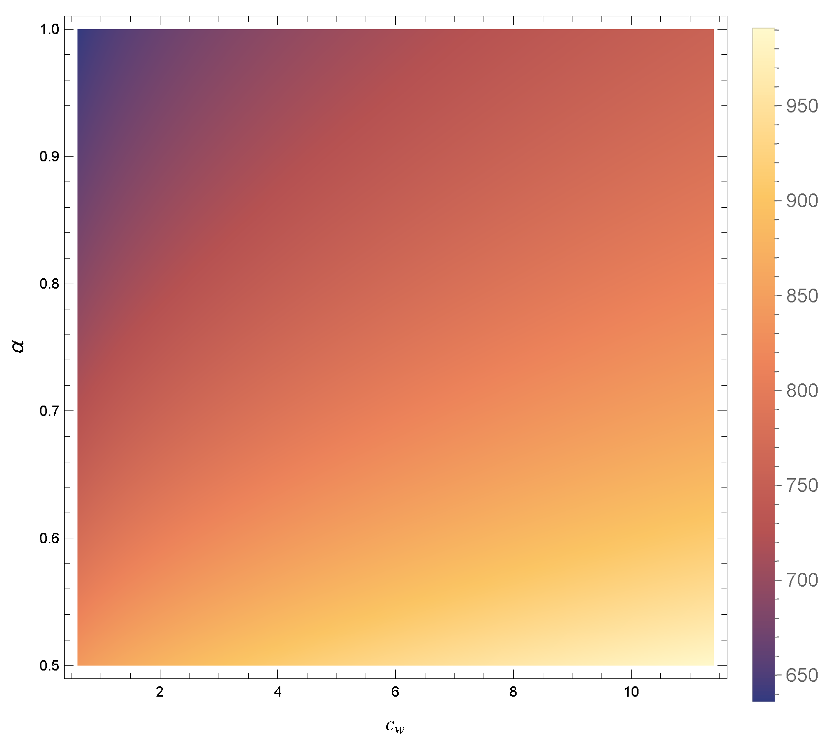
To complement the discrete sweep results reported in Table 1 and Table 2, we visualize the dependence of the optimized expected total cost on the waiting-cost parameter and the phase-speed structure by means of a two-dimensional heatmap.

Specifically, for each pair $(c_w,\alpha )$, we compute the optimal traffic intensity level

$${\rho }^{*}(c_w,\alpha )=arg\underset{\rho \in (0,1)}{min}\mathsf{\Phi }(\rho ;\alpha ,c_w),$$

and plot the corresponding minimized cost value $\mathsf{\Phi }\left({\rho }^{*}(c_w,\alpha )\right)$ as a color-coded surface over the domain

$$c_w\in [0.6,11.4],\alpha \in [0.5,1].$$

This representation provides a continuous sweep map of the optimal operating cost with respect to both the waiting-cost weight and the service-phase speed structure. The two tables correspond to horizontal cross-sections of this surface at $\alpha =0.5$ and $\alpha =1$, respectively.

The heatmap therefore compactly summarizes the combined effect of cost weighting and phase heterogeneity on system performance, allowing the main sweep trends to be identified visually without relying on large numerical tables.

The heatmap in Figure 1 shows that the optimal expected total cost $\mathsf{\Phi }\left({\rho }^{*}\right)$ increases monotonically with the waiting cost parameter $c_w$ and with decreasing values of the phase-speed factor $\alpha$. Lower cost levels are concentrated in the region of small $c_w$ and $\alpha$ close to 1, corresponding to balanced service speeds across phases. In contrast, heterogeneous service speeds ($\alpha <1$) lead to systematically higher costs for the same waiting-cost level. Overall, the figure confirms that $c_w$ is the dominant driver of cost growth, while $\alpha$ governs the relative efficiency of the system within the feasible operating region.

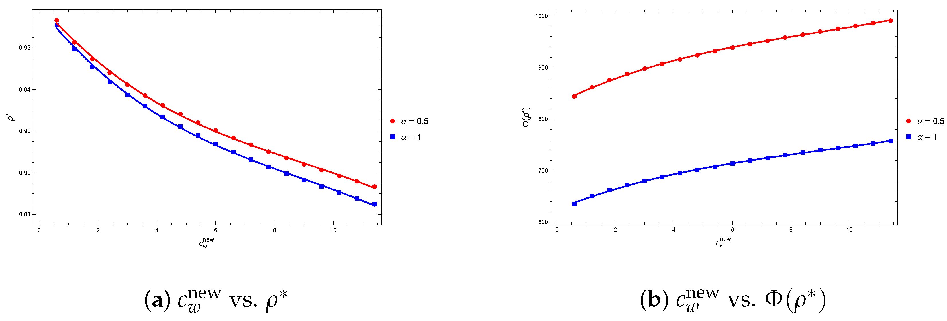
Polynomial Trend Fitting for Optimal Solutions

As an auxiliary summary of the monotone dependence observed in Table 1 and Table 2, we fit third-degree polynomial regressions describing how the optimal traffic intensity ${\rho }^{*}$ and the optimal expected total cost $\mathsf{\Phi }\left({\rho }^{*}\right)$ vary with $c_w^{\mathrm{new}}$. The estimated coefficients (with standard errors, test statistics, and p-values) are reported in

Table 3. Polynomial regression results for ${\rho }^{*}$ and $\mathsf{\Phi }\left({\rho }^{*}\right)$ for various $c_w^{\mathrm{new}}$ values.

Term	Estimate	Standard Error	t-Statistic	p-Value	Decision for ${\mathit{H}}_0$
$c_w^{\mathrm{new}}$ vs. ${\rho }^{*},\alpha =0.5$
1	0.981131	0.000767175	1278.89	$3.3483\times {10}^{-39}$	Reject
x	$-0.0163009$	0.0005395	$-30.2148$	$7.4830\times {10}^{-15}$	Reject
$x^2$	0.0013055	0.000103079	12.665	$2.0613\times {10}^{-9}$	Reject
$x^3$	$-0.000048789$	$5.6560\times {10}^{-6}$	$-8.62612$	$3.3636\times {10}^{-7}$	Reject
$c_w^{\mathrm{new}}$ vs. ${\rho }^{*},\alpha =1$
1	0.979444	0.000836274	1171.2	$1.2527\times {10}^{-38}$	Reject
x	$-0.017625$	0.000588093	$-29.9697$	$8.4399\times {10}^{-15}$	Reject
$x^2$	0.00141699	0.000112364	12.6107	$2.1870\times {10}^{-9}$	Reject
$x^3$	$-0.0000530003$	$6.1654\times {10}^{-6}$	$-8.59642$	$3.5133\times {10}^{-7}$	Reject
$c_w^{\mathrm{new}}$ vs. $\mathsf{\Phi }\left({\rho }^{*}\right),\alpha =0.5$
1	830.163	1.24044	669.25	$5.5388\times {10}^{-35}$	Reject
x	28.0223	0.872314	32.1241	$3.0244\times {10}^{-15}$	Reject
$x^2$	$-2.10786$	0.166668	$-12.6471$	$2.1019\times {10}^{-9}$	Reject
$x^3$	0.0785848	0.00914509	8.59311	$3.5304\times {10}^{-7}$	Reject
$c_w^{\mathrm{new}}$ vs. $\mathsf{\Phi }\left({\rho }^{*}\right),\alpha =1$
1	624.616	1.0103	618.249	$1.8188\times {10}^{-34}$	Reject
x	22.9995	0.710472	32.3722	$2.6989\times {10}^{-15}$	Reject
$x^2$	−1.72485	0.135746	−12.7064	$1.9705\times {10}^{-9}$	Reject
$x^3$	0.0643556	0.00744838	8.64021	$3.2950\times {10}^{-7}$	Reject

for both $\alpha =0.5$ and $\alpha =1$.

In Table 3, the independent variable is $c_w^{\mathrm{new}}$ and is denoted by x for brevity (the same convention is used later for ${(c_1+\alpha c_2)}_{new}$ or $2c_{\mathrm{new}}$). For each coefficient ${\beta }_i$, we test $H_0:{\beta }_i=0$ against $H_1:{\beta }_i\ne 0$. At conventional significance levels (e.g., $0.05$ or $0.01$), all reported p-values satisfy $\alpha >$p-Value; hence, $H_0$ is rejected for every term. The corresponding fitted curves are shown in Figure 2.

Table 4. Model evaluation metrics for polynomial fits of $c_w^{\mathrm{new}}$ vs. ${\rho }^{*}$ and $c_w^{\mathrm{new}}$ vs. $\mathsf{\Phi }\left({\rho }^{*}\right)$, for $\alpha =0.5$ and $\alpha =1$.

Metric	${\mathit{\rho }}^{*}$$(\mathit{\alpha }=0.5)$	${\mathit{\rho }}^{*}$$(\mathit{\alpha }=1)$	$\mathsf{\Phi }\left({\mathit{\rho }}^{*}\right)$$(\mathit{\alpha }=0.5)$	$\mathsf{\Phi }\left({\mathit{\rho }}^{*}\right)$$(\mathit{\alpha }=1)$
$R^2$	0.999312	0.999295	0.999475	0.999487
Adjusted $R^2$	0.999174	0.999153	0.99937	0.999385
MAE	0.000492462	0.000532089	0.797367	0.649684
MSE	$3.6172\times {10}^{-7}$	$4.2981\times {10}^{-7}$	0.945649	0.627304
RMSE	0.000601429	0.000655599	0.972445	0.792025
MAPE (%)	0.0527691	0.0573089	0.0875073	0.0940157
Max Error	0.00148982	0.0016324	2.41499	1.96821

summarizes the fit quality. All models achieve $R^2>0.999$ (and similarly high adjusted $R^2$). The errors are small: for ${\rho }^{*}$, the RMSE is $0.000601429$ ($\alpha =0.5$) and $0.000655599$ ($\alpha =1$); for $\mathsf{\Phi }\left({\rho }^{*}\right)$, the MAE is below 1 and the RMSE is $0.972445$ ($\alpha =0.5$) and $0.792025$ ($\alpha =1$). The relative errors are also very small (MAPE below $0.1\%$ in all cases). Overall, third-degree polynomials provide accurate compact approximations of the numerically obtained optimal solutions over the tested range of $c_w^{\mathrm{new}}$.

6.3. Sweep and Statistical Analysis Based on Changes in the Amortization Cost Parameters $c_1$, $c_2$, and c

In this subsection, we present experimental results for both sweep and statistical analyses in which the amortization costs are varied simultaneously in accordance with the relation $c_1+\alpha c_2=2c$.

For the first case ($\alpha =0.5$), we select the initial values $c_1=12$ and $c_2=8$, which yield ${(c_1+\alpha c_2)}_{\mathrm{initial}}=16$. We then vary this quantity according to the rate

$$\Delta (c_1+\alpha c_2):0\%,\pm 10\%,\dots ,\pm 90\%$$

relative to ${(c_1+\alpha c_2)}_{\mathrm{initial}}$, and we compute the corresponding new values

$${(c_1+\alpha c_2)}_{\mathrm{new}}={(c_1+\alpha c_2)}_{\mathrm{initial}}+\Delta (c_1+\alpha c_2).$$

For the second case ($\alpha =1$), we choose the initial value $c_{\mathrm{initial}}=8$, which implies $2c_{\mathrm{initial}}=16$. The new values are then obtained as

$$2c_{\mathrm{new}}=2c_{\mathrm{initial}}+\Delta 2c,$$

where

$$\Delta 2c:0\%,\pm 10\%,\dots ,\pm 90\%$$

is defined relative to $2c_{\mathrm{initial}}$.

All remaining parameters are held fixed throughout the experiments, namely $\lambda =25$, $p=0.5$, and $c_w=6$. The numerical results are reported in

Table 5. Optimal traffic intensity, optimal service speeds and optimal expected total cost for different ${(c_1+\alpha c_2)}_{\mathrm{new}}$ for $\alpha =0.5$.

$\mathsf{\Delta }({\mathit{c}}_1+\mathit{\alpha }{\mathit{c}}_2)$	${({\mathit{c}}_1+\mathit{\alpha }{\mathit{c}}_2)}_{\mathbf{new}}$	${\mathit{\rho }}^{*}$	${\mathit{\mu }}_1^{*}$	${\mathit{\mu }}_2^{*}$	$\mathsf{\Phi }\left({\mathit{\rho }}^{*}\right)$
$-90\%$	1.6	0.7850	63.69	31.85	123.82
$-80\%$	3.2	0.8378	59.68	29.84	221.97
$-70\%$	4.8	0.8635	57.91	28.95	315.89
$-60\%$	6.4	0.8796	56.85	28.42	407.64
$-50\%$	8	0.8909	56.12	28.06	497.98
$-40\%$	9.6	0.8994	55.59	27.80	587.33
$-30\%$	11.2	0.9062	55.18	27.59	675.93
$-20\%$	12.8	0.9117	54.84	27.42	763.94
$-10\%$	14.4	0.9163	54.56	27.28	851.45
$0\%$	16	0.9203	54.33	27.17	938.56
$+10\%$	17.6	0.9237	54.13	27.06	1025.33
$+20\%$	19.2	0.9267	53.95	26.98	1111.79
$+30\%$	20.8	0.9294	53.80	26.90	1197.99
$+40\%$	22.4	0.9318	53.66	26.83	1283.95
$+50\%$	24	0.9340	53.54	26.77	1369.71
$+60\%$	25.6	0.9359	53.42	26.71	1455.27
$+70\%$	27.2	0.9377	53.32	26.66	1540.67
$+80\%$	28.8	0.9394	53.23	26.61	1625.90
$+90\%$	30.4	0.9409	53.14	26.57	1710.99

for $\alpha =0.5$ and in

Table 6. Optimal traffic intensity, optimal service speed and optimal expected total cost for different $2c_{\mathrm{new}}$ for $\alpha =1$.

$\mathsf{\Delta }2\mathit{c}$	$2{\mathit{c}}_{\mathbf{new}}$	${\mathit{\rho }}^{*}$	${\mathit{\mu }}^{*}$	$\mathsf{\Phi }\left({\mathit{\rho }}^{*}\right)$
$-90\%$	1.6	0.7697	48.72	96.29
$-80\%$	3.2	0.8256	45.42	171.15
$-70\%$	4.8	0.8530	43.96	242.54
$-60\%$	6.4	0.8701	43.10	312.13
$-50\%$	8	0.8823	42.50	380.59
$-40\%$	9.6	0.8914	42.07	448.23
$-30\%$	11.2	0.8987	41.73	515.26
$-20\%$	12.8	0.9046	41.46	581.80
$-10\%$	14.4	0.9096	41.23	647.94
$0\%$	16	0.9138	41.04	713.75
$+10\%$	17.6	0.9175	40.87	779.27
$+20\%$	19.2	0.9207	40.73	844.55
$+30\%$	20.8	0.9236	40.60	909.61
$+40\%$	22.4	0.9262	40.49	974.48
$+50\%$	24	0.9285	40.39	1039.18
$+60\%$	25.6	0.9306	40.30	1103.73
$+70\%$	27.2	0.9325	40.21	1168.13
$+80\%$	28.8	0.9343	40.14	1232.41
$+90\%$	30.4	0.9360	40.07	1296.57

for $\alpha =1$.

Specifically, Table 5 contains the percentage change of $c_1+\alpha c_2$, which is denoted by $\Delta (c_1+\alpha c_2)$, the new value ${(c_1+\alpha c_2)}_{new}$, the optimal traffic intensity ${\rho }^{*}$, the optimal service speed in the first phase

$${\mu }_1^{*}={\displaystyle \frac{\lambda (\alpha +p)}{\alpha {\rho }^{*}}},$$

the optimal service speed in the second phase ${\mu }_2^{*}=\alpha {\mu }_1^{*}$, and the corresponding optimal value of the cost function (16), denoted by $\mathsf{\Phi }\left({\rho }^{*}\right)$.

Similarly, Table 6 reports the percentage change of $2c$, denoted by $\Delta 2c$, the new value $2c_{\mathrm{new}}$, the optimal traffic intensity ${\rho }^{*}$, the optimal service speed

$${\mu }^{*}={\displaystyle \frac{\lambda (1+p)}{{\rho }^{*}}},$$

and the optimal value of the cost function (17), $\mathsf{\Phi }\left({\rho }^{*}\right)$.

Effect of Changes in ${({\mathit{c}}_{\mathbf{1}}+\mathit{\alpha }{\mathit{c}}_{\mathbf{2}})}_{\mathbf{new}}$ and $\mathbf{2}{\mathit{c}}_{\mathbf{new}}$. For $\alpha =0.5$, reducing $(c_1+\alpha c_2)$ by $90\%$ from the baseline ${(c_1+\alpha c_2)}_{\mathrm{initial}}=16$ decreases the optimal traffic intensity ${\rho }^{*}$ by about 15%, increases the optimal service speeds ${\mu }_1^{*}$ and ${\mu }_2^{*}$ by roughly 17%, and reduces the expected total cost $\mathsf{\Phi }\left({\rho }^{*}\right)$ by approximately 87%. Conversely, increasing the cost by $90\%$ raises ${\rho }^{*}$ by about 2.5%, reduces service speeds by about 2.2%, and increases $\mathsf{\Phi }\left({\rho }^{*}\right)$ by about 82.3%.

For $\alpha =1$, a $90\%$ decrease in $2c_{new}$ leads to a slightly stronger response: ${\rho }^{*}$ decreases by about 15.8%, ${\mu }^{*}$ increases by about 18.7%, and $\mathsf{\Phi }\left({\rho }^{*}\right)$ decreases by roughly 86.5%. A $90\%$ increase produces the opposite effect: ${\rho }^{*}$ rises by about 2.5%, ${\mu }^{*}$ falls by about 2.4%, and $\mathsf{\Phi }\left({\rho }^{*}\right)$ increases by about 81.6%. Thus, amortization-cost changes strongly affect both traffic intensity and service speeds, while cost variations remain substantial in both directions and for both models.

Operational efficiency.Table 5 and Table 6 show that the traffic intensity increases as amortization costs rise in both models, reflecting reduced service effort when capacity becomes more expensive. However, the $\alpha =0.5$ model consistently requires higher service speeds than the single speed ${\mu }^{*}$ under $\alpha =1$, indicating more intensive service operation. Moreover, cost increases are steeper for $\alpha =0.5$, whereas the $\alpha =1$ configuration exhibits smoother cost growth and lower service effort. Overall, $\alpha =1$ provides higher operational efficiency and greater cost stability under varying amortization costs.

Further trend insights. Both models exhibit smooth, convex cost behavior consistent with Theorem 2 with traffic intensity increasing monotonically as amortization costs rise. While both adapt gradually to cost changes, the $\alpha =0.5$ configuration shows stronger sweep in $\mathsf{\Phi }\left({\rho }^{*}\right)$, indicating lower robustness to cost perturbations. In contrast, $\alpha =1$ yields smoother cost trajectories and more stable service speeds.

Overall, although both models adjust effectively to amortization-cost variation, the $\alpha =1$ configuration provides more stable and predictable performance with lower sweep and smoother cost evolution. The $\alpha =0.5$ model remains more responsive but also more volatile, which may complicate cost control. These results highlight the advantage of $\alpha =1$ as a more robust and economically stable operating regime under changing amortization conditions.

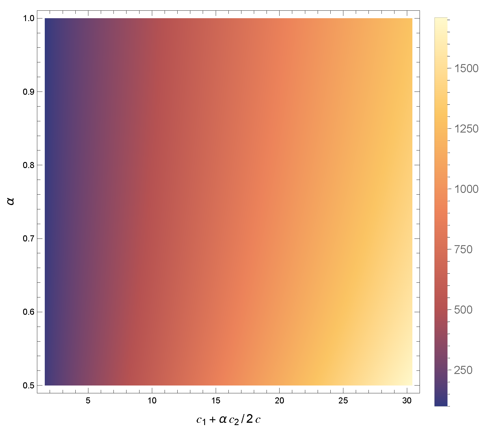
To further improve the interpretability of the sweep results reported in Table 5 and Table 6, we complement the tabulated numerical values with a two–dimensional heatmap representation. The heatmap depicts the optimal expected total cost $\mathsf{\Phi }\left({\rho }^{*}\right)$ as a function of the comparable amortization term ${(c_1+\alpha c_2)}_{\mathrm{new}}$ (or $2c_{\mathrm{new}}$) and the phase–speed factor $\alpha$. This visualization provides a compact overview of the joint impact of amortization costs and service-speed heterogeneity on the system’s cost structure and facilitates the identification of regions associated with low and high operating costs. The heatmap is shown in Figure 3.

The heatmap illustrates that the optimal expected total cost $\mathsf{\Phi }\left({\rho }^{*}\right)$ increases monotonically with the amortization cost parameter $c_1+\alpha c_2$ (or $2c$), as evidenced by the pronounced left-to-right color gradient. For a fixed amortization level, larger values of $\alpha$, corresponding to more balanced service speeds across phases, consistently result in lower expected total costs, which is visible as darker regions toward the upper part of the plot. Hence, amortization costs constitute the dominant driver of overall cost growth, whereas the phase-speed structure primarily governs cost efficiency with configurations closer to $\alpha =1$ being systematically more economical.

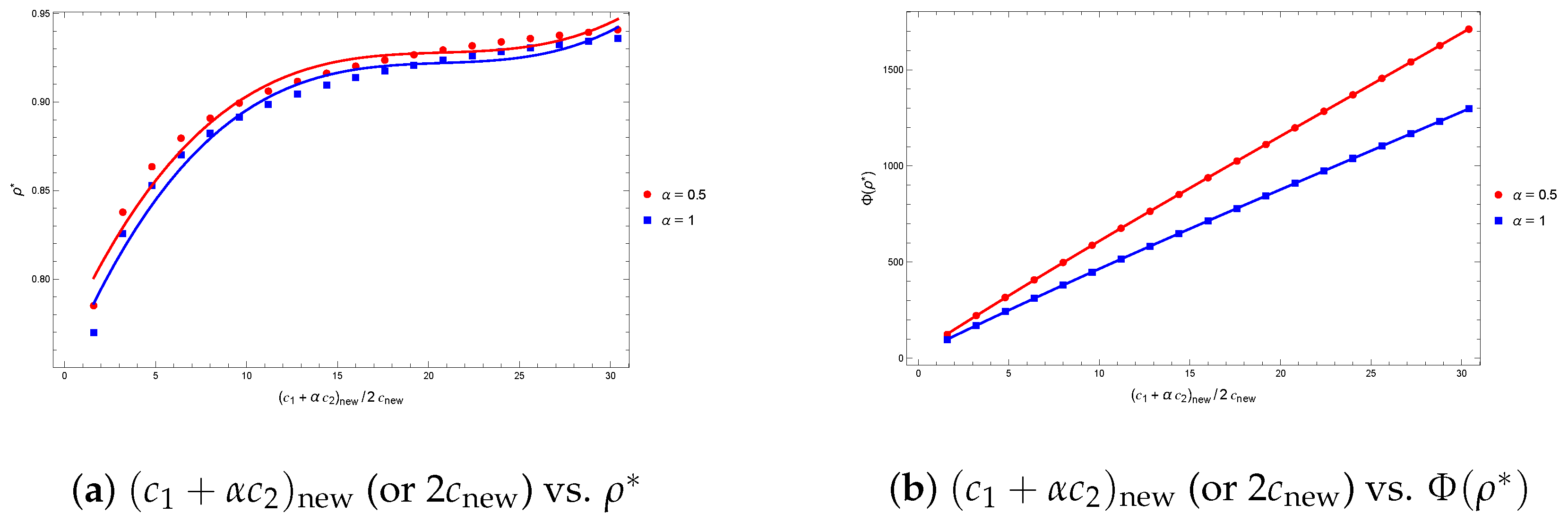
Polynomial Trend Fitting for Optimal Solutions

To provide a compact statistical summary of the sweep results in Table 5 and Table 6, we fit third-degree polynomial regressions linking the amortization-related parameter ${(c_1+\alpha c_2)}_{\mathrm{new}}$ for $\alpha =0.5$ (or equivalently $2c_{new}$ for $\alpha =1$) to the optimal solutions ${\rho }^{*}$ and $\mathsf{\Phi }\left({\rho }^{*}\right)$. The estimated coefficients are reported in

Table 7. Polynomial regression results for ${\rho }^{*}$ and $\mathsf{\Phi }\left({\rho }^{*}\right)$ for various ${(c_1+\alpha c_2)}_{\mathrm{new}}$ (or $2c_{\mathrm{new}}$) values.

Term	Estimate	Standard Error	t-Statistic	p-Value	Decision for ${\mathit{H}}_0$
${(c_1+\alpha c_2)}_{\mathrm{new}}$ vs. ${\rho }^{*},\alpha =0.5$
1	0.767148	0.007635	100.4770	$1.2354\times {10}^{-22}$	Reject
x	0.022659	0.002013	11.2538	$1.0342\times {10}^{-8}$	Reject
$x^2$	$-0.001079$	0.000144	$-7.4790$	$1.9535\times {10}^{-6}$	Reject
$x^3$	0.00001737	$2.9684\times {10}^{-6}$	5.8517	$3.1848\times {10}^{-5}$	Reject
${(c_1+\alpha c_2)}_{\mathrm{new}}$ vs. $\mathsf{\Phi }\left({\rho }^{*}\right),\alpha =0.5$
1	0.750531	0.008040	93.3489	$3.7191\times {10}^{-22}$	Reject
x	0.024104	0.002120	11.3686	$9.0162\times {10}^{-9}$	Reject
$x^2$	$-0.001146$	0.000152	$-7.5405$	$1.7702\times {10}^{-6}$	Reject
$x^3$	0.00001842	$3.1258\times {10}^{-6}$	5.8940	$2.9482\times {10}^{-5}$	Reject
$2c_{\mathrm{new}}$ vs. ${\rho }^{*},\alpha =1$
1	30.16345	1.24044	24.3168	$1.8279\times {10}^{-13}$	Reject
x	60.50837	0.32712	184.9744	$1.3162\times {10}^{-26}$	Reject
$x^2$	$-0.29642$	0.02344	$-12.6471$	$2.1019\times {10}^{-9}$	Reject
$x^3$	0.004144	0.0004823	8.5931	$3.5304\times {10}^{-7}$	Reject
$2c_{\mathrm{new}}$ vs. $\mathsf{\Phi }\left({\rho }^{*}\right),\alpha =1$
1	25.12360	1.01702	24.7031	$1.4509\times {10}^{-13}$	Reject
x	46.09814	0.26820	171.8796	$3.9575\times {10}^{-26}$	Reject
$x^2$	$-0.24294$	0.01922	$-12.6425$	$2.1124\times {10}^{-9}$	Reject
$x^3$	0.003399	0.0003954	8.5965	$3.5129\times {10}^{-7}$	Reject

. As before, for each coefficient, we test $H_0:{\beta }_i=0$ against $H_1:{\beta }_i\ne 0$; all reported p-values are below common significance levels; hence, all terms are statistically significant.

The fitted polynomial relationships are illustrated in Figure 4.

Table 8. Model evaluation metrics for polynomial fits of ${(c_1+\alpha c_2)}_{\mathrm{new}}$ (or $2c_{\mathrm{new}}$) vs. ${\rho }^{*}$ and ${(c_1+\alpha c_2)}_{\mathrm{new}}$ (or $2c_{\mathrm{new}}$) vs. $\mathsf{\Phi }\left({\rho }^{*}\right)$, for $\alpha =0.5$ and $\alpha =1$.

Metric	${\mathit{\rho }}^{*}$$(\mathit{\alpha }=0.5)$	${\mathit{\rho }}^{*}$$(\mathit{\alpha }=1)$	$\mathsf{\Phi }\left({\mathit{\rho }}^{*}\right)$$(\mathit{\alpha }=0.5)$	$\mathsf{\Phi }\left({\mathit{\rho }}^{*}\right)$$(\mathit{\alpha }=1)$
$R^2$	0.976832	0.977476	0.999996	0.999995
Adj. $R^2$	0.972198	0.972972	0.999995	0.999994
MAE	0.0047567	0.00501346	0.797367	0.653177
MSE	$3.5827\times {10}^{-5}$	$3.9728\times {10}^{-5}$	0.945649	0.635682
RMSE	0.00598552	0.00630303	0.972445	0.797297
MAPE (%)	0.542169	0.577749	0.218553	0.232559
Max Error	0.0157115	0.0165409	2.41499	1.98262

reports standard fit diagnostics. For ${\rho }^{*}$, the explanatory power remains high ($R^2=0.976832$ for $\alpha =0.5$ and $R^2=0.977476$ for $\alpha =1$) with an MAE of $0.0047567$–$0.00501346$ and RMSE of $0.00598552$–$0.00630303$ (MAPE below $0.6\%$). For $\mathsf{\Phi }\left({\rho }^{*}\right)$, the fits are nearly exact ($R^2>0.99999$) with RMSE values of $0.972445$ ($\alpha =0.5$) and $0.797297$ ($\alpha =1$) and an MAPE below $0.25\%$. Overall, cubic polynomials provide accurate, low-parameter approximations of the numerically optimized ${\rho }^{*}$ and $\mathsf{\Phi }\left({\rho }^{*}\right)$ as functions of the amortization-cost level.

6.4. Difference-Based Evaluation: Wilcoxon Signed-Rank Test

To quantify the effect of the phase-structure parameter $\alpha$, we compare the optimal solutions under $\alpha =0.5$ and $\alpha =1$ via the paired differences

$$\Delta {\rho }^{*}={\rho }_{\alpha =0.5}^{*}-{\rho }_{\alpha =1}^{*},\Delta \mathsf{\Phi }\left({\rho }^{*}\right)=\mathsf{\Phi }{\left({\rho }^{*}\right)}_{\alpha =0.5}-\mathsf{\Phi }{\left({\rho }^{*}\right)}_{\alpha =1}.$$

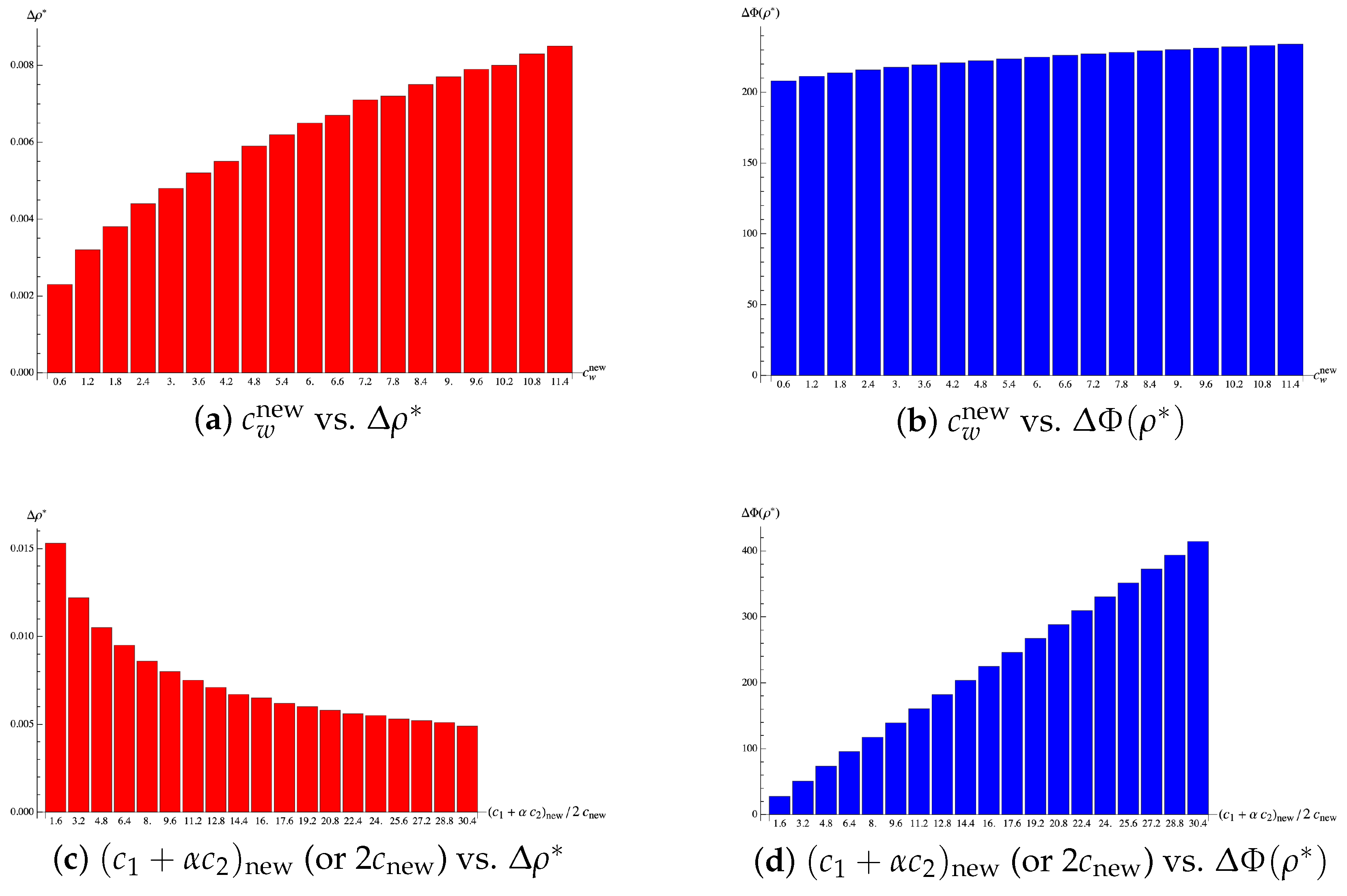
The distributions of $\Delta {\rho }^{*}$ and $\Delta \mathsf{\Phi }\left({\rho }^{*}\right)$ are displayed in Figure 5: panels (a)–(b) correspond to the sweep runs in Table 1 and Table 2 (varying $c_w^{\mathrm{new}}$), while panels (c)–(d) correspond to Table 5 and Table 6 (varying ${(c_1+\alpha c_2)}_{\mathrm{new}}=2c_{\mathrm{new}}$). In all panels, red bars represent $\Delta {\rho }^{*}$ and blue bars represent $\Delta \mathsf{\Phi }\left({\rho }^{*}\right)$.

To test whether these paired differences are statistically different from zero, we apply the Wilcoxon signed-rank test (paired, two-sided). Using $n=19$ paired observations in each comparison, all differences are strictly positive in Figure 5a–d. The test yields $W=190$ and $p=0.00014$, so for $H_0$, the median difference equaling zero, is rejected at the 5% level for both $\Delta {\rho }^{*}$ and $\Delta \mathsf{\Phi }\left({\rho }^{*}\right)$ under both the $c_w^{\mathrm{new}}$-variation and the amortization-cost-variation experiments. Therefore, $\alpha =1$ systematically achieves smaller optimal traffic intensity and lower optimized expected total cost than $\alpha =0.5$ across the considered parameter ranges, indicating a more efficient operating regime.

7. Conclusions

In this paper, we proposed a general and analytically tractable cost function formulation for the $M/Co{x}_k(p_1,\dots ,p_{k-1};{\mu }_1,\dots ,{\mu }_k)/1$ queueing system with customer service speed variability. A parametric representation of phase-dependent service speeds enabled explicit analytical expressions for key performance measures, including expected waiting time, system size, and total operational cost. The cost function was formulated in terms of the traffic intensity $\rho$, and its convexity was proven, ensuring the existence and uniqueness of the optimal value ${\rho }^{*}$. Numerical experiments confirmed the theoretical results and illustrated how optimal solutions vary under changes in waiting and amortization cost parameters.

The sweep analysis shows that the configuration with $\alpha =1$ consistently provides superior performance. Across all tested parameter ranges, it yields lower optimal expected total costs $\mathsf{\Phi }\left({\rho }^{*}\right)$, lower optimal traffic intensity ${\rho }^{*}$, and smoother cost responses, indicating greater stability and predictability. In contrast, heterogeneous service speeds ($\alpha <1$) do not improve cost efficiency and instead lead to higher traffic intensity levels and steeper cost growth, particularly under increasing cost pressures. From an operational standpoint, constant service speeds support more stable and cost-effective system management. Although variable service speeds may arise in practice, the results indicate that balanced service configurations provide more favorable trade-offs between cost, performance, and robustness.

By linking service speed structure to operational costs, the model provides clear guidance for system design and resource allocation. Maintaining consistent service speeds across phases reduces expected costs while improving predictability and stability, offering actionable insights for optimizing multi-phase service systems in areas such as healthcare, manufacturing, and service operations.

8. Limitations and Further Research Directions

The proposed model relies on several assumptions that ensure analytical tractability but also indicate directions for further research. The main limitations are summarized below.

• Single-server structure. The system is modeled as a single-server queue, which may be restrictive for large-scale or parallel service environments. Future work may extend the model to tandem or multi-server queueing networks to better capture complex operational settings.
• Sequential phase entry. All customers are assumed to enter at phase 1 and proceed sequentially. In practice, customers may enter at intermediate stages or require only partial processing. Extensions with probabilistic phase entry and routing would broaden the model’s applicability.
• Linear cost structure. Costs are assumed to be linear in waiting and service-capacity components. However, standard, nonlinear cost functions may better capture congestion effects, technological constraints, or economies of scale, and thus these represent an important direction for future work.
• Structured service speeds. Service rates are assumed to follow a geometric progression ${\mu }_i={\mu }_1{\alpha }^{i-1}$, $i=1,\dots ,k$. While this provides a compact parameterization, it may be restrictive in systems with heterogeneous technologies or resources. More flexible structures, such as independently specified or data-driven service speeds, could improve realism.
• Sweep-based analysis. This paper uses sweep analysis rather than formal quantitative sensitivity measures. Future research may incorporate differential sensitivity metrics and uncertainty-based approaches, such as Monte Carlo simulations, to assess robustness more rigorously.
• Optimization formulation. Optimization is performed with respect to the traffic intensity $\rho$ to preserve convexity and analytical tractability. An alternative approach is to express cost directly in terms of arrival and service rates, enabling the use of metaheuristic or global optimization methods for more complex or nonconvex extensions.

These directions provide a basis for developing more flexible and realistic cost-aware queueing models while preserving the core analytical insights established in this work.