Article

A Mathematical Model for Type 1 Diabetes Regulation Using a Smart Insulin Patch: In Silico Validation Based on Published Rat Data


Department of Mathematics, Jamoum University College, Umm Al-Qura University, Makkah 24320, Saudi Arabia
Math. Comput. Appl. 2026, 31(2), 41; https://doi.org/10.3390/mca31020041
Submission received: 15 December 2025 / Revised: 23 February 2026 / Accepted: 4 March 2026 / Published: 5 March 2026

Abstract

This work introduces a new mathematical model designed to describe the glucose–insulin dynamics associated with a glucose-responsive smart microneedle patch reported in the literature. The model captures the complete sequence of the patch behavior, from detecting glucose changes to controlled transdermal insulin delivery and gradually restoring blood glucose levels to the normal range. Our simulations show that the patch can effectively manage glucose not only during fasting conditions but also after single and multiple meals, restoring glucose levels to healthy levels within a short period. The model predictions are consistent with experimentally reported trends in previously published studies, which strengthens confidence in the biological realism of the proposed mechanism. Because some parameters in such systems are difficult to measure directly, we also performed a comprehensive sensitivity analysis to understand how variations in key parameters influence system stability. The results highlight the central role of the insulin release rate and the five glucose–regulation parameters examined in the sensitivity analysis, providing clear guidance on the most critical aspects of patch design for reliable performance. Overall, this study provides a simplified yet robust mathematical framework that makes the behavior of a glucose-responsive microneedle patch easy to understand and analyze. It lays the groundwork for future refinement of control strategies and optimization of patch design, improving control strategies, and developing more advanced systems that can maintain healthy glucose levels naturally and intuitively.

1. Introduction

Diabetes is an autoimmune disease characterized by impaired insulin production, leading to elevated blood glucose levels and affecting various systems in the body [1,2,3]. There are several types of diabetes, including Type 1 diabetes (T1D), Type 2 diabetes (T2D), and gestational diabetes [4,5]. Type 1 diabetes (T1D) occurs when the immune system mistakenly destroys the insulin-producing β -cells located in the islets of Langerhans in the pancreas [5,6,7,8,9]. In contrast, Type 2 diabetes (T2D) develops when the body’s cells become resistant to insulin, and the pancreas gradually produces less of it over time [6,7]. Many people can manage or improve this condition through lifestyle changes along with medication. Gestational diabetes, on the other hand, appears during pregnancy, when hormonal shifts reduce the body’s sensitivity to insulin, leading to higher blood glucose levels [6,7].
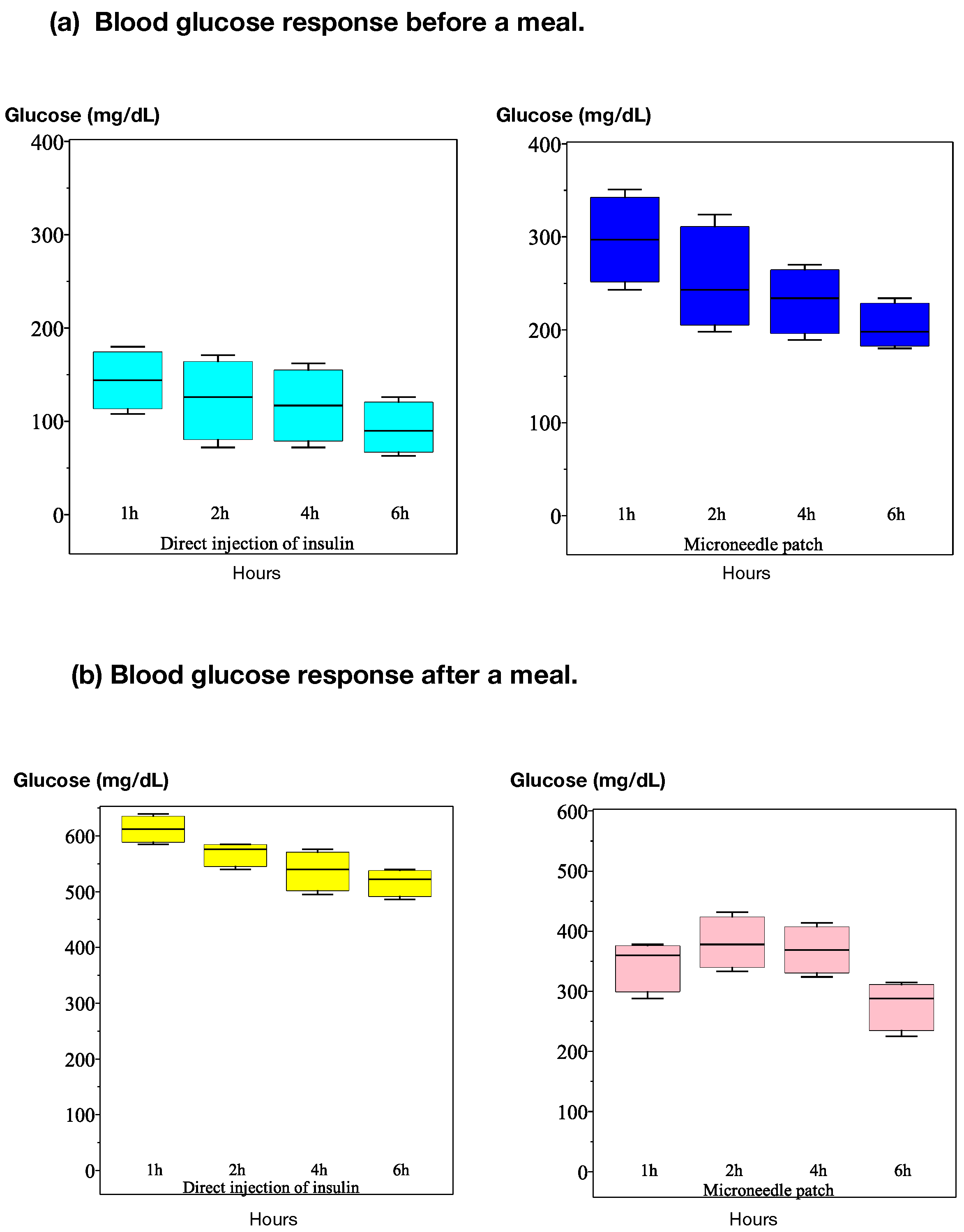
Many researchers focus on diabetes to discover more effective treatment options (for example, [10,11,12,13,14]). There are also many studies looking for new and creative ways to treat diabetes, including research on glucose-responsive microneedle-array patches reported in the literature that can sense glucose levels and release insulin automatically when the body needs it [15,16,17,18,19]. This microneedle patch shows a clear experimentally validated biological effect, because it senses when glucose levels rise and releases insulin to help bring them back to normal [20,21,22]. Ongoing research continues to advance the development of smart microneedle patches. A recent study published in 2023, Tan et al. [19], showed that the smart microneedle patch could lower blood glucose in rats with type 1 diabetes (T1D), both before and after meals, and compared its effect to traditional insulin injections (see Figure 1).
It is important to emphasize that the glucose-responsive microneedle patch considered in this study is not newly developed by the authors. Instead, the proposed model is formulated based on a biologically validated smart microneedle patch previously reported in the literature, particularly the experimental work of Tan et al. [19]. In these systems, insulin is typically encapsulated within glucose-sensitive polymeric or vesicular matrices embedded in microneedles. Elevated glucose levels trigger insulin release through mechanisms such as polymer swelling, enzymatic reactions, or changes in local pH, enabling controlled and on-demand delivery. Critical formulation factors include insulin loading capacity, glucose sensitivity threshold, polymer composition, microneedle geometry, and diffusion-controlled release kinetics, all of which influence the effectiveness and stability of the delivery system [15,19,20].
Building on recent advances in biological sciences and the emergence of smart therapeutic technologies, this work aims to develop a mathematical model that helps us understand how a smart insulin patch reported in the literature can improve blood glucose regulation. The model is designed to examine the effect of the patch under both fasting and post-meal conditions, clarify the mechanism by which this technology operates, and assess its ability to regulate glucose more efficiently and in a gentler, more responsive manner that aligns with the body’s needs. For this reason, we aim to develop a mathematical model that focuses on the dynamics of the microneedle patch’s effect on blood glucose levels and provide a theoretical demonstration that supports and reproduces the experimental outcomes reported by Tan et al. [19].
In contrast to existing glucose–insulin models that primarily describe diabetes progression or conventional insulin administration strategies, the present work introduces a mathematical framework specifically designed to capture the dynamics of glucose-responsive microneedle-based insulin delivery. Unlike traditional models, which often assume instantaneous or continuous insulin input, the proposed model explicitly incorporates glucose-triggered, delayed, and controlled insulin release through the skin. This allows the model to represent the sensing–response mechanism of smart microneedle patches and to analyze their impact on blood glucose regulation under both fasting and postprandial conditions, including multiple meal scenarios. Such features are not explicitly addressed in existing modeling approaches, thereby highlighting the novelty and relevance of the proposed framework.
Many mathematical models describe the process of diabetes [23,24,25,26,27], and others have been developed to describe the glucose–insulin regulatory dynamics in type 1 or type 2 diabetes [28,29,30,31]. In addition, several mathematical models have been proposed to simulate and evaluate different treatment strategies for diabetes, including insulin therapy, glucose-responsive systems, and drug-delivery approaches [32,33,34]. To keep pace with recent advances in diabetes treatments, new therapeutic approaches have continued to evolve, including smart microneedle patches that release insulin when glucose levels rise. These patches have shown better glucose control than traditional methods [15,19], making them a promising option for the future. Because of this progress, researchers have also started using mathematical models to understand how these patches work, especially how insulin moves from the patch into the skin and then into the bloodstream. Some mathematical models describe the movement and distribution of microneedle patches across different compartments [35,36,37]. However, the present work focuses specifically on modeling the impact of microneedle-based insulin delivery on systemic blood glucose dynamics, rather than on patch fabrication or transport mechanisms. In addition, the model reflects the microneedle patch’s ability to reduce glucose levels, consistent with the experimental trends reported by Tan et al. [19]. Moreover, we investigate the system response under multiple-meal scenarios and present simulations demonstrating a reduction in glucose levels to approximately 73 mg/dL by the end of 100 h (≈4 days).
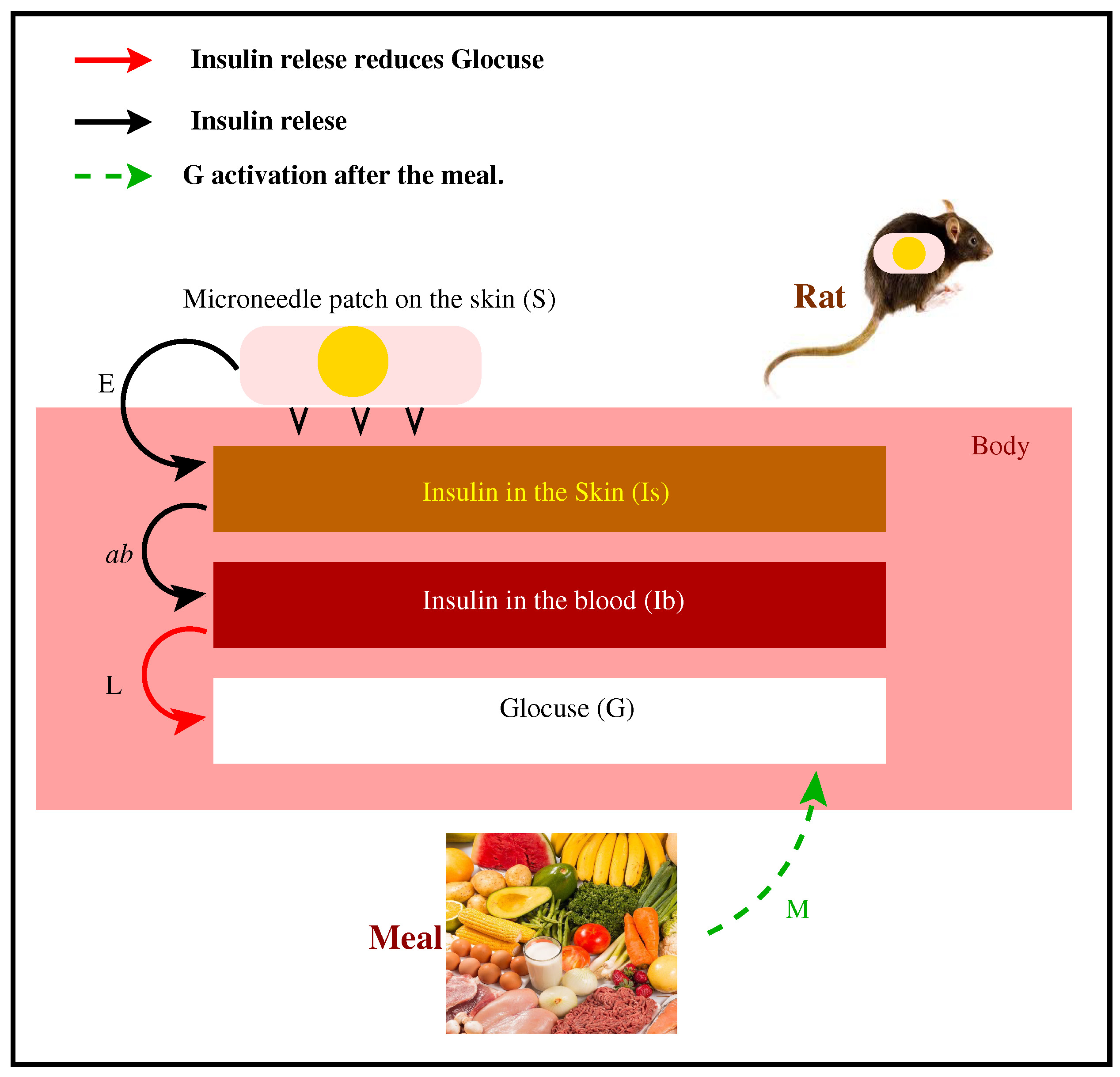
We develop a novel mathematical framework that focuses on how a microneedle patch adopted from existing experimental studies works through the skin: how it senses rising glucose, releases insulin into the skin layer, and gradually lowers blood glucose. In addition, the model captures the natural rise in glucose after meals and how the patch responds to it (see Figure 2). The results indicate that the patch keeps glucose under control, bringing it back to normal levels after both short- and long-term meal challenges. We also compare our results with those of Tan et al. [19] at fasting and post-meal times, and observe good agreement with published experimental measurements. Since some of the parameters are unknown and based on assumptions, a sensitivity analysis is performed to examine how they influence the model behavior.
Figure 1. Schematic illustration adapted from [19] comparing conventional insulin injection and a glucose-responsive microneedle patch in a rat model: (a) blood glucose response before a meal and (b) blood glucose response after a meal. In both cases, the microneedle patch was applied approximately 6 h before or after meal intake.
Mca 31 00041 g001
Figure 2. Insulin delivery mechanism of the smart microneedle patch. Insulin is first released into the skin compartment and then absorbed into the second compartment (the bloodstream), where it exerts its glucose-lowering effect. The figure also illustrates the impact of a meal on glucose dynamics in the rat.
Mca 31 00041 g002
The paper is organized as follows. Section 2 outlines the mathematical framework. Section 3 analyzes the model behavior (Section 3.2), including steady-state characterization (Section 3.1) and a global sensitivity analysis (Section 4), which assesses the impact of the parameter on Glucose dynamics over 12 and 24 h. Section 5 concludes with a summary and discussion.

2. Glucose Dynamics Under Microneedle Patch Influence

In this study, we investigated a simplified mathematical model to describe the dynamics of glucose under the influence of a microneedle patch. The insulin density in the patch is denoted by S, the insulin within the skin compartment by I s , the insulin in the bloodstream by I b , and the glucose concentration by G. The following system of differential equations governs the temporal evolution of these variables:
d S d t = S E ,
d I s d t = S E e s I s a b I s ,
d I b d t = a b I s e b I b ,
d G d t = L + a G G ( 1 G m ) e G G + M .
In the following section, we describe in detail the terms that appear in model (1).
  • In Equation (1a), the patch releases insulin at the rate E is defined as a piecewise function that activates only when glucose exceeds a threshold. When glucose is below 120 mg/dL [38], the patch does not release insulin E = 0 . However, once glucose is reached or higher than 120 mg/dL, the patch releases insulin, which follows a saturating Michaelis–Menten-type response. The parameter k s represents the maximum possible release rate achieved when glucose is sufficiently high [21]. In contrast, the parameter k m determines the glucose level at which the release reaches half of this maximum, analogous to a half-saturation constant in enzyme-mediated glucose-responsive systems [39]. This glucose-dependent release is represented by the following function:
    E = 0 , G < 120 , k s G k m + G , G 120 ,
  • In Equation (1b), after the patch releases insulin at the rate k s   S E [40,41], the insulin enters the skin compartment, where it is cleared at the rate e s [42], and remaining insulin then moves from the skin into the bloodstream at the transfer rate a b [43].
  • In Equation (1c), after insulin leaves the skin, it enters the bloodstream at the rate a b [44,45], and part of the insulin may remain in the skin and not enter the bloodstream immediately due to local degradation or tissue binding [46,47]. Thus, the insulin is naturally cleared at a rate e b .
  • In Equation (1d), glucose also follows logistic growth due to production from other cells in the body at a rate a g [48] approaching a carrying capacity m [49,50]. Moreover, the body still clears some glucose naturally through normal metabolism, physical activity, and hydration. These processes continue to lower glucose levels even without insulin or medication [51,52]. Thus, glucose is naturally cleared at a rate e g , and it is further reduced by insulin released from the microneedle patch at the rate n g [15,49,53]. The combined glucose-dependent insulin-release term L is modeled as a piecewise stimulus that activates only when glucose exceeds a physiologically meaningful threshold. When blood glucose is below 120 mg/dL, the smart microneedle patch remains inactive and releases no insulin:
    L = 0 , G < 120 , n g G I b , G 120
We focus on two distinct states: the fasting state before the meal (Fast, M = 0 ) and the post-meal state (M). The time bounds used in the definition of M are modeling assumptions introduced to represent meal events over finite time windows. These intervals do not correspond to the exact duration of eating, but rather approximate physiologically reasonable postprandial periods during which glucose enters the bloodstream. This assumption allows a simplified and tractable representation of meal-induced glucose input while preserving the essential dynamics of the system. In the case of a single meal, only one value of M is considered at 20 min:
M = 0 , t < 0.16 , 1 , 0.16 t < 0.17 , 0 , t 0.17
Here, the time variable t represents a normalized (dimensionless) time obtained by scaling the physical time with respect to a characteristic time scale of the system. Accordingly, the interval 0.16 t < 0.17 corresponds to a short postprandial window of approximately 20 min in real time. During this interval, the function M is set to M = 1 to represent the presence of a meal and the associated glucose input. Outside this interval, M = 0 , corresponding to the fasting state. Thus, the values t < 0.16 and t < 0.17 are used to distinguish the pre-meal, meal, and post-meal phases within the early-time dynamics.
In the multiple meal scenario, the multiple post-meal values of (M) are introduced at 5 h, 15 h, and 22 h:
M = 0 , t < 5 , 1 , 5 t < 6 , 0 , 6 t < 15 , 1 , 15 t < 16 , 0 , 16 t < 22 , 1 , 22 t < 23 , 0 , t 23 .
In the multi-meal scenario, the function M represents discrete postprandial glucose inputs rather than continuous insulin release. Accordingly, M = 1 only during the specified meal intervals (e.g., 5 t < 6 ), indicating the presence of glucose intake. For t < 5 and 6 t < 15 , no new glucose input is introduced ( M = 0 ). During these intervals, insulin is not actively triggered by a meal; however, the system dynamics still reflect the residual effect of previously released insulin through its interaction with glucose and other state variables.

3. Results

Now, we investigate a model (1) by analyzing its equilibrium points, which characterize the system’s long-term behavior and provide insight into its underlying stability structure. In the steady-state analysis, the absence of insulin simply indicates that the patch is inactive because glucose levels are already low, so no release is required. When glucose rises, however, the patch activates and begins delivering insulin, helping the system return to a healthier equilibrium. This contrast clearly shows how the patch distinguishes between low and high glucose states.

3.1. Steady States and Stability

We now focus only on the two steady states that can realistically occur in the body, since they are the only ones that make biological sense. We analyze the long-term behavior of model (1) by examining its steady-state dynamics.
  • In the absence of insulin and in the continued presence of glucose, the system admits an equilibrium of the form ( S , I s , I b , G ) = ( 0 , 0 , 0 , G * ) , representing a physiological state in which glucose persists at a baseline level. At the same time, the microneedle patch does not produce insulin. Under the baseline parameter values listed in Table A1, this equilibrium is classified as locally asymptotically stable. The general stability properties of this state are established in Appendix B. The corresponding equilibrium glucose concentration is given by
    G * = m a G ( a G e G ) which exists only when ( a G > e G ) .
  • In the presence of both insulin and glucose, the system admits a non-trivial equilibrium of the form ( S , I s , I b , G ) = ( S * , I s * , I b * , G * ) . Under the baseline parameter values given in Table A1, this steady state is non-zero and is classified as stable. The equilibrium components satisfy the following:
S * = k m + G * k s G * ( e s a b ) I s * which exists only when ( e s > a b ) , I s * = e b a b I b * , I b * = a b e b I s * , G * = m ( 1 n g I b * + e G a G ) which exists only when ( 1 > n g I b * + e G a G ) ,

3.2. Numerical Results

We show how glucose behaves before the meal and after the post-meal phase to highlight how the system changes in response to eating. We assume the initial condition G ( 0 ) = 378 mg/dL [19]. This value is chosen to represent a moderate-to-high hyperglycemic state. Clinically, postprandial glucose targets are typically below ∼180 mg/dL, whereas glucose levels exceeding 300 mg/dL are commonly regarded as markedly elevated and indicative of poor glycemic control. Moreover, severe hyperglycemia has been reported in the clinical literature at levels above 400 mg/dL. Therefore, the value 378 mg/dL (approximately 21 mmol/L) provides a physiologically relevant initial condition that is substantially above recommended targets while remaining below extreme emergency thresholds, making it suitable for evaluating the performance of the patch under pronounced hyperglycemic stress. The value S ( 0 ) = 3  μU/mL represents the initial insulin density in the patch [19], corresponding to the amount of insulin stored in the patch before activation. In addition, I s ( 0 ) = 0 represents the amount of insulin in the skin compartment at the start of the simulation, indicating that no insulin has yet been delivered from the patch into the skin at time t = 0 . Similarly, I b ( 0 ) = 0 denotes the insulin concentration in the bloodstream at the beginning of the simulation, since insulin release from the patch is triggered only when glucose levels become elevated. Thus, the initial conditions G ( 0 ) = 378 mg/dL, S ( 0 ) = 3  μU/mL, I s ( 0 ) = 0 , and I b ( 0 ) = 0 represent a moderate hyperglycemic state prior to patch activation.

3.2.1. Pre-Meal (Fasting, M = 0 ) Phase

In Figure 3, we present the simulation of glucose levels before the meal: panel (a) shows the short-term behavior over 12 h, panel (b) illustrates the long-term behavior over 24 h, and panel (c) compares the numerical results of the glucose levels with experimental data from rats over 6 h. It can be clearly seen that glucose levels decrease when the patch is applied. This reduction occurs because the patch releases insulin when glucose levels are high, and the released insulin subsequently lowers the glucose level. The model captures the overall trend of the experimental data reported by Tan et al. [19], showing close agreement at 1 h, 2 h, and 6 h. Although the predicted value at 4 h is slightly lower than the experimental range, the deviation remains modest and biologically reasonable.

3.2.2. Post-Meal Phase

In this section, we show the post-meal simulation for the first 20 min to illustrate the immediate glucose response after food intake. Then, we illustrated the results of three-meal simulations conducted at hours 5, 15, and 22 to analyze the system’s longer-term behavior.
Single Meal Introduced Early in the Day
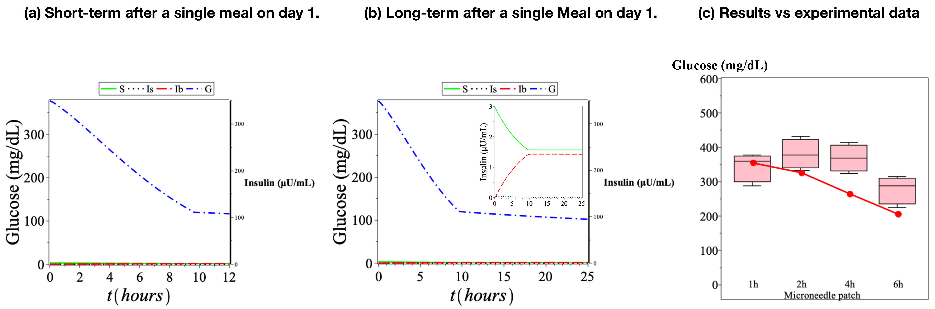
In Figure 4, we illustrate the simulation of glucose levels after a meal: panel (a) shows the short-term behavior over 12 h, panel (b) illustrates the long-term behavior over 24 h, and panel (c) compares the numerical results of the glucose levels with experimental data from rats over 6 h. It can be clearly seen that glucose levels decrease when the patch is applied. This reduction occurs because the patch releases insulin when glucose levels are high, and the released insulin subsequently lowers the glucose level. The model and the experimental data show the same behavior. The model fits the data of Tan et al. [19] exactly at 1 h and 2 h, and remains close at 6 h. Although the 4 h value is slightly lower than the experimental range, the deviation is modest and remains within an acceptable biological range.
Although Figure 3 and Figure 4 correspond to pre-meal and post-single-meal conditions, respectively, their trajectories appear visually similar. This observation may seem counterintuitive, as meal intake is expected to induce a transient rise in glucose levels. To clarify this behavior and avoid potential misinterpretation, we quantitatively compare the model predictions at selected time points using Table 1. Table 1 reports the predicted glucose levels for both scenarios at 1, 2, 4, and 6 h. The results show that, while the meal introduces a short-lived postprandial perturbation, the glucose-responsive microneedle patch rapidly compensates for this disturbance. Consequently, glucose dynamics quickly converge to the same regulated trajectory, explaining the strong visual overlap observed in Figure 3 and Figure 4.
Multiple-Meals Scenario on Day One
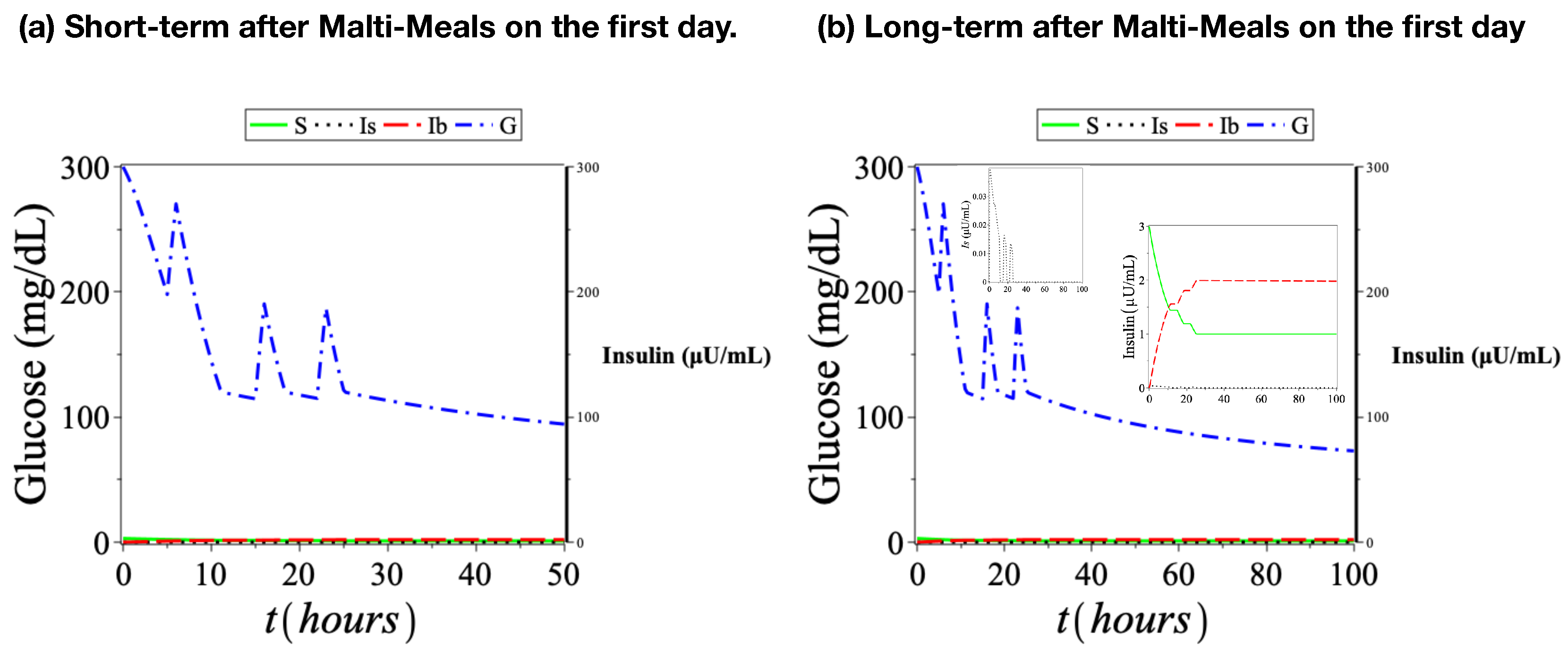
In Figure 5, we show how glucose changes after three post-meal events. In panel (a), we see the short-term behavior over 50 h (≈2 days), and in panel (b), the long-term behavior over 100 h (≈4 days). When the patch is applied, glucose levels begin to fall because it releases insulin when glucose levels rise. After 5 h, the first meal causes glucose to rise, but the patch quickly responds by releasing insulin, bringing the level back to normal within about 2–3 h. The same pattern occurs at 15 h: glucose increases after the second meal, and the patch again releases insulin, returning glucose to normal within a few hours. A third rise appears at hour 22, and once more the patch lowers glucose back to normal in about 2–3 h. This third glucose peak is associated with the third meal explicitly introduced in the model through the function M ( t ) , where glucose input is activated during the interval 22 t < 23 . After this point, glucose remains stable at around 73 mg/dL for the rest of the (≈4) days.
When comparing the system under fasting with a single meal versus multiple meals, we observe that glucose levels rise after each meal, and the patch responds by releasing insulin to bring the glucose back to its normal range within a few hours. Despite the repeated meals, the system maintains stable glucose levels, demonstrating the effectiveness of the patch in controlling these frequent fluctuations.

4. Sensitivity Analysis

To better understand the relative influence of the model parameters on the system dynamics, a sensitivity analysis was carried out. By systematically varying each parameter around its baseline value, we quantify how sensitive the state variables are to small perturbations in the parameters. This approach allows us to identify which biological processes exert the strongest control over the glucose and insulin dynamics at equilibrium and during the transient phase.
To measure the influence of each model parameter on the output, an anxiety-based global sensitivity analysis was performed. For any parameter p, a sensitivity interval of ± 10% around its nominal value was defined. Within this interval, N = 50 uniformly spaced samples were generated. Let p min and p max denote the lower ( 10% ) and upper ( + 10% ) bounds of the interval. The step size is computed as Δ p = p max p min N 1 , and the sampled values are defined by
p i = p min + ( i 1 ) Δ p , i = 1 , 2 , , N
For each sampled value p i , the model was simulated, and the resulting output (e.g., G ( 12 ) and G ( 24 ) ) was recorded. The variation in the output across the 50 simulations was then used to compute sensitivity indices and rank the parameters according to their influence on model behavior, following standard global sensitivity analysis methodologies. We selected the unknown parameters for the sensitivity analysis to check how much they influence the model and to ensure that the values we assumed for them are reasonable and correct.
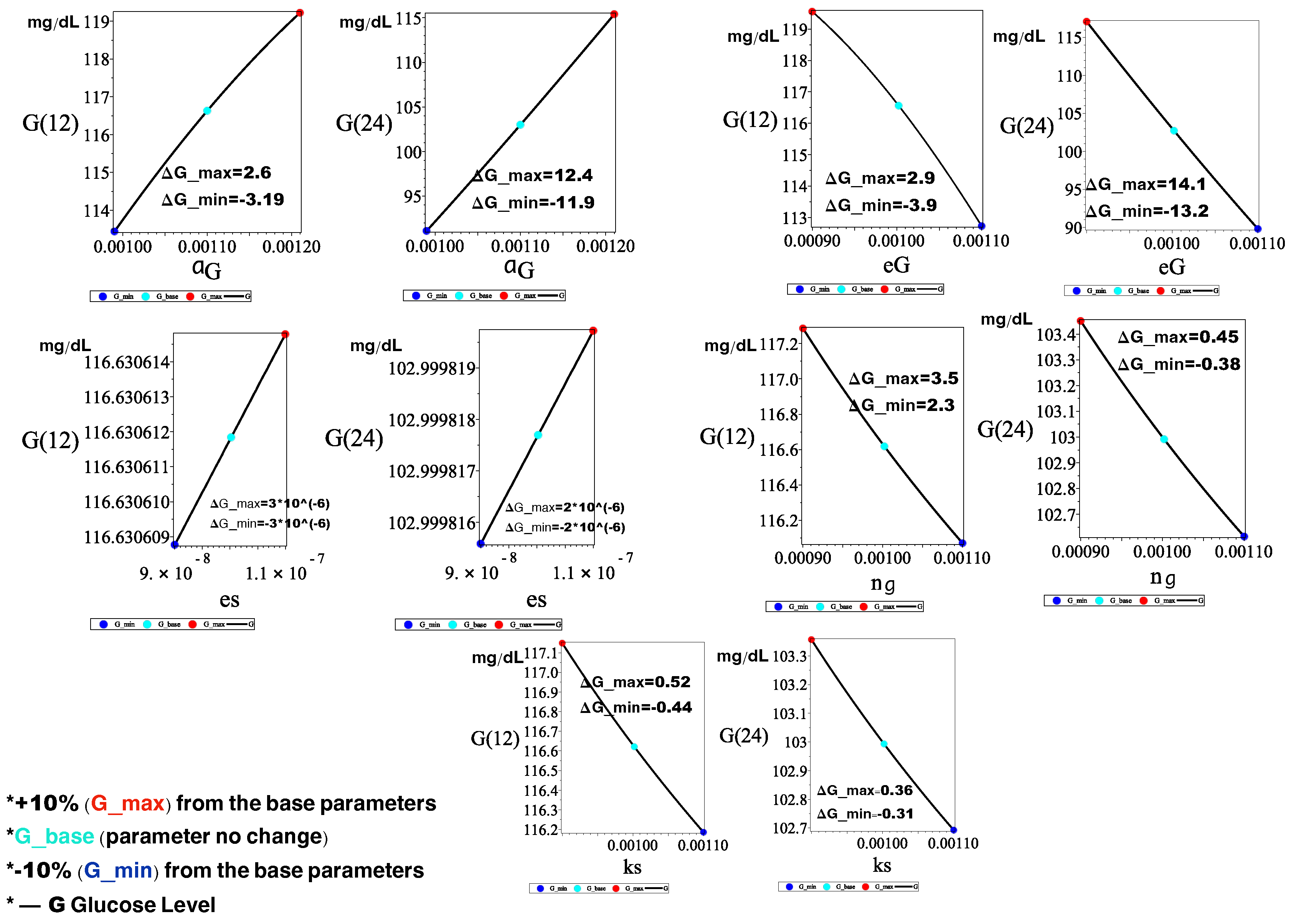
Figure 6 presents the global sensitivity analysis of model 1 before the meal, where each parameter was perturbed by ± 10% over a two-hour (12 h and 24 h). The parameters tested include the insulin release rate from the patch ( k s ), the natural decay rate of insulin in the skin ( e s ), the natural decay rate of glucose ( e G ), the glucose growth rate ( a G ), and the glucose elimination rate via insulin ( n g ).
The results illustrate that, for most parameters, the resulting variation in the evaluated outputs ( G ( 12 ) and G ( 24 ) ) is very small. This indicates that the model is relatively robust with respect to moderate uncertainties in these parameters. In contrast, the parameters e G and a G display a noticeably stronger influence. Perturbing e G and a G within the same ± 10% range produces a substantially larger change in the model outputs compared with the other parameters, highlighting their dominant roles in shaping the system dynamics. This behavior, in which only a small subset of parameters contributes significantly to output variability, is consistent with findings from other biological dynamical models employing global sensitivity analysis.
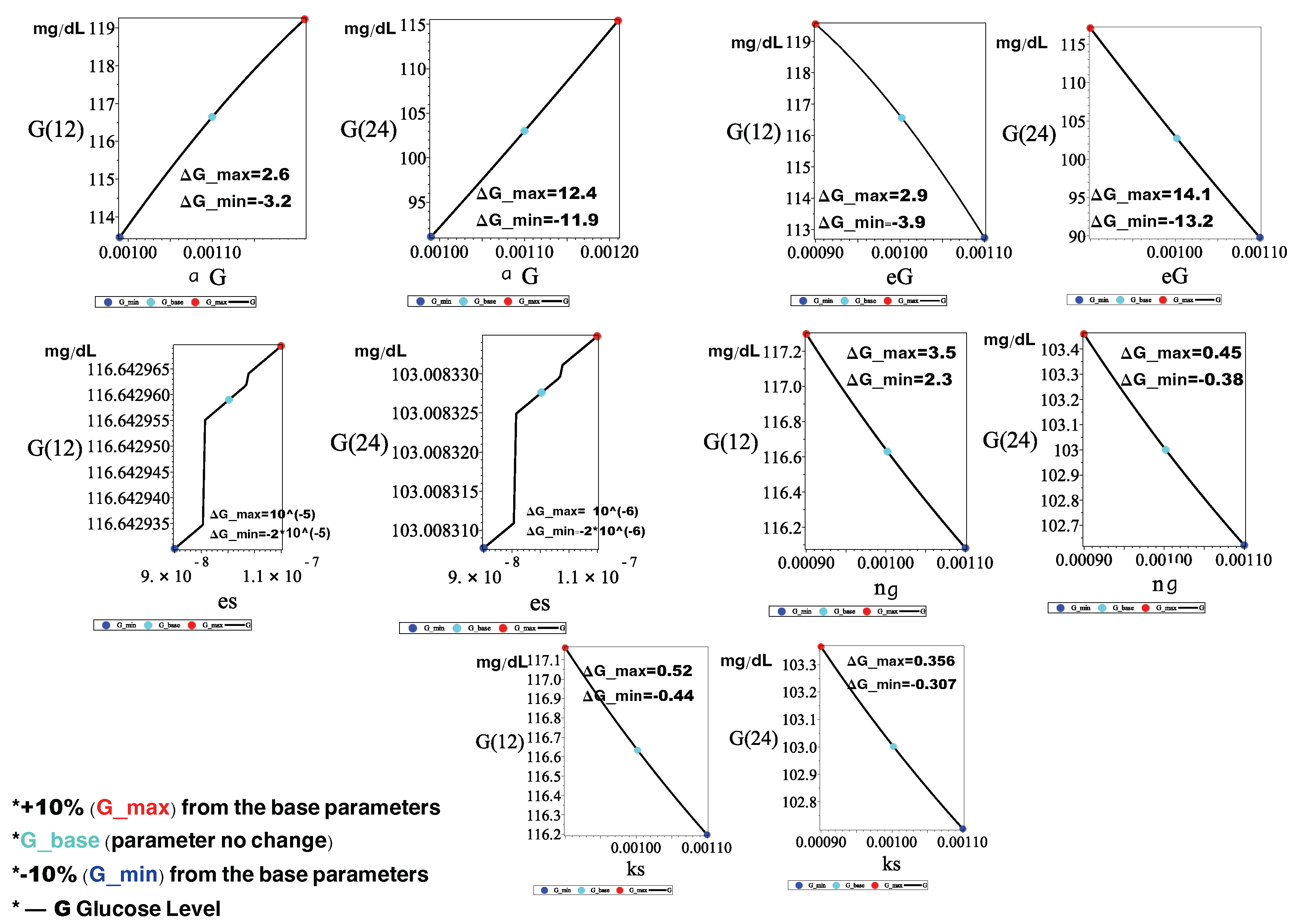
Figure 7 shows the global sensitivity analysis of model (1) after the meal, where each parameter was perturbed by ± 10% over a two-hour (12 h and 24 h). The parameters tested include the insulin release rate from the patch ( k s ), the natural decay rate of insulin in the skin ( e s ), the natural decay rate of glucose ( e G ), the glucose growth rate ( a G ), and the glucose elimination rate via insulin ( n g ).
Overall, the analysis shows that most parameters induce only minimal variation in the evaluated outputs, G ( 12 ) and G ( 24 ) . This indicates that the model is generally robust to moderate uncertainties in these parameter values. However, two parameters e G and a G display a noticeably stronger impact. Perturbing these parameters within the same ± 10% interval results in substantially larger changes in the model output compared with the other parameters, underscoring their key roles in shaping the system’s behavior. sensitivity analysis.
Figure 6. The figure shows the global sensitivity analysis before the meal, based on ± 10% perturbations of the parameters k s , e s , n g , e G , and a G .
Mca 31 00041 g006
Figure 7. The figure shows the global sensitivity analysis after the meal, based on ± 10% perturbations of the parameters k s , e s , n g , e G , and a G .
Mca 31 00041 g007
It is also worth noting that the global sensitivity profiles were almost unchanged before and after the meal. The parameter perturbations resulted in almost the same output variations at both time points (12 h and 24 h), indicating that the model’s sensitivity structure is stable across feeding conditions. This consistency further demonstrates the robustness of the model and shows that the dominant influence of e G and a G persists whether the system is evaluated in the pre-meal or post-meal state.
The multi-meal scenario involves repeated meal inputs without altering the underlying model parameters; therefore, the parameter sensitivity structure remains unchanged, and a separate sensitivity analysis is not expected to provide additional insight.

5. Conclusions

The results of our model show that the smart microneedle patch does more than simply release insulin; it behaves like a responsive system that understands when glucose begins to rise and adjusts its release accordingly. In our simulations, even before/after one or multiple meals, glucose levels returned smoothly to the normal range without sharp spikes or drops, demonstrating the patch’s ability to maintain stable control throughout realistic daily conditions.
Another important point is the strong agreement between our simulated glucose curves and the experimental data reported [19] in previous studies during both the fasting and post-meal periods. This close match suggests that the model successfully captures the essential physiological interactions between glucose, insulin, and the skin-based delivery mechanism. It also provides confidence that the assumptions made in the model are biologically reasonable.
Because some parameters are not yet well characterized experimentally, we performed a comprehensive global sensitivity analysis to test how variations in key parameters affect model behavior. The results highlight that parameters such as the insulin release rate, the natural decay of insulin in the skin, and the glucose elimination rate have a substantial influence on the system’s stability. This insight is important for real-world development: it shows which parameters must be measured more exactly and which aspects of patch design are most critical for achieving reliable glucose control.
Future work will focus on refining the mathematical structure of the model by incorporating more realistic delay terms, improving the representation of glucose appearance after meals, and exploring alternative functional forms for insulin diffusion through the skin.
Overall, this study provides a practical mathematical framework for understanding how a glucose-responsive microneedle patch behaves in real-life scenarios. It demonstrates that such a patch can, in principle, regulate glucose effectively throughout the day, while also identifying the key factors that will need careful attention in future experimental and clinical development.

Funding

This research received no external funding.

Data Availability Statement

No new data were created or analyzed in this study. Data sharing is not applicable to this article.

Conflicts of Interest

The author declares no conflicts of interest.

Appendix A. Parameter Estimation

The parameter values used in the model (1) are summarized in Table A1.
Table A1. Table summarizing the parameters that appear in the model (1).
Param.DescriptionValueUnitsRef.
k s The rate of insulin release from the patch 10 3 10 1 ( 10 3 )h−1Estimation
k m Glucose concentration producing half-maximal insulin release126–162 (120)mg/dLEstimation
a b Insulin rate moves from the skin into the bloodstream.0.05h−1[54]
mCarrying capacity of the glucose451–750 (600)mg/dL[55]
e s The nature decay rate of the insulin in skin 10 8 10 4 ( 10 7 )h−1Estimation
e b The nature decay rate of the insulin in bloodstream 10 8 10 4 ( 10 6 )h−1[54]
e G The nature decay rate of the glucose 10 4 –0.001 ( 10 3 )h−1Estimation
a G The growth rate of the glucose 10 4 –0.05 (0.0011)h−1Estimation
n g The elimination rate of the glucose via insulin 10 4 –0.05 ( 10 3 )(μU/mL)−1 h−1Estimation

Estimation of the Rate

  • Insulin release rate from the patch: We assumed the insulin release parameter from the patch within a biologically reasonable range; no single value is firmly established in the literature. Nevertheless, published studies consistently show that proteins diffuse through microneedle-treated skin at a slow to moderate rate, typically on the order of ( 10 3 10 1 ) h−1 [47].
  • Glucose concentration producing half-maximal insulin release: Although no study reports an explicit half-maximal glucose concentration for insulin release from glucose-responsive microneedle patches [21,56], published data consistently show a typical sigmoidal-like release pattern, characterized by minimal insulin release at normoglycemia and a steep rise under hyperglycemic conditions. Based on this qualitative behavior, we adopt a working assumption of (126–162) mg/dL.
  • Nature elimination rate of the insulin in skin: Since the skin does not significantly break down insulin, and most clearance occurs in the liver and kidneys [57], there are no direct measurements of insulin decay in skin tissue. For this reason, we model insulin loss in the skin using a very small decay range (10−4 10 8 ) h−1, reflecting that degradation in this compartment is minimal.
  • Natural elimination rate of glucose: In streptozotocin-induced diabetic rats, natural glucose disposal is substantially weakened, leading to impaired tissue uptake and prolonged periods of hyperglycemia [58]. To reflect this markedly diminished insulin-independent clearance in our simulations, we assume a small effective removal rate of 10 3 h−1 in the model.
  • Elimination rate of glucose via microneedle patches: The microneedle patches release insulin slowly and steadily, not like fast injections, and studies show that absorption from these patches is gradual [59]. Thus, we assume a small insulin-driven glucose elimination rate ( 10 3 ) (μU/mL)−1 h−1 to reflect this controlled delivery.
  • Growth rate of the glucose: We use a small glucose growth rate ( 10 3 ) h−1 because the body can naturally raise blood glucose even without food intake. Hormones such as glucagon and cortisol stimulate the liver to produce glucose, but this increase is slow and limited, so a small value appropriately represents this basal glucose rise in the model [48].
We will perform a sensitivity analysis because these parameters are only an estimate, not an experimentally measured value, and we want to make sure the model stays stable and does not change too much when the parameter varies.

Appendix B. Stability of Steady States

In the following, we briefly focus on the stability of the four types of steady states described in Section 3.1. The Jacobian matrix associated with the system (1) is:
J = c 11 c 12 c 13 c 14 c 21 c 22 c 23 c 24 c 31 c 32 c 33 c 34 c 41 c 42 c 43 c 44
where
c 11 = k s G * k m + G * , c 12 = 0 , c 13 = 0 , c 14 = k s S * ( k m + G * ) 2 , c 21 = k s G * k m + G * , c 22 = e s e b , c 23 = 0 , c 24 = k s S * ( k m + G * ) 2 , c 31 = 0 , c 32 = a b , c 33 = e s , c 34 = 0 , c 41 = 0 , c 42 = 0 , c 43 = n g G * , c 44 = a G 1 2 G * m e G n g I b * .
Proposition A1.
Consider the system (1). The trivial steady state ( S , I s , I b , G ) = ( 0 , 0 , 0 , G * ) is stable or unstable.
Proof. 
In ( S , I s , I b , G ) = ( 0 , 0 , 0 , G * ) the Jacobian matrix is
J ( 0 , 0 , 0 , G * ) = c 11 c 12 c 13 c 14 c 21 c 22 c 23 c 24 c 31 c 32 c 33 c 34 c 41 c 42 c 43 c 44
c 11 = k s G * k m + G * , c 12 = 0 , c 13 = 0 , c 14 = 0 , c 21 = k s G * k m + G * , c 22 = e s e b , c 23 = 0 , c 24 = 0 , c 31 = 0 , c 32 = a b , c 33 = e s , c 34 = 0 , c 41 = 0 , c 42 = 0 , c 43 = n g G * , c 44 = a G 1 2 G * m e G
λ 1 = k s G * k m + G * < 0 , λ 2 = e s e b < 0 , λ 3 = e s < 0 , λ 4 = e G a G ( 1 2 G * m ) .
Therefore, the sign of λ 4 determines the stability of the trivial steady state. The equilibrium is locally asymptotically stable if
e G < a G 1 2 G * m ,
and unstable if
e G > a G 1 2 G * m .
In the boundary case
e G = a G 1 2 G * m ,
the linearization is inconclusive, and higher-order analysis is required.
For the trivial equilibrium G * = 0 , we have 2 G * m = 0 < 1 , and thus λ 4 = e G a G , implying stability if e G < a G and instability if e G > a G . □
Proposition A2.
For any initial condition ( S ( 0 ) , I s ( 0 ) , I b ( 0 ) , G ( 0 ) ) R + 4 , system (1) admits a unique solution ( S ( t ) , I s ( t ) , I b ( t ) , G ( t ) ) defined for all t 0 . Moreover, the solution remains non-negative and bounded for all t 0 .
Proof. Step 1: Existence and uniqueness (local).
Let X ( t ) = ( S ( t ) , I s ( t ) , I b ( t ) , G ( t ) ) T and write (1) as
X ˙ = F ( X ) , X ( 0 ) = X 0 R + 4 .
Since the components of F are continuously differentiable functions of ( S , I s , I b , G ) on R + 4 (hence F is locally Lipschitz on bounded sets), the Picard–Lindelöf theorem guarantees that for each X 0 there exists a unique maximal solution X ( t ) on [ 0 , T max ) , where T max ( 0 , ] .
Step 2: Positivity (invariance of R + 4 ). Define
t 0 = inf t > 0 : S ( t ) < 0 or I s ( t ) < 0 or I b ( t ) < 0 or G ( t ) < 0 .
Assume by contradiction that t 0 < T max . Then all components are non-negative on [ 0 , t 0 ] and at least one component reaches 0 at t = t 0 .
Using (1a)–(1d) and the fact that all variables are non-negative on [ 0 , t 0 ] , we obtain the lower differential inequalities
S ˙ ( t ) E S ( t ) , I ˙ s ( t ) ( e s + a b ) I s ( t ) ,
I ˙ b ( t ) e b I b ( t ) , G ˙ ( t ) e G G ( t ) , t t 0 .
By the comparison principle,
S ( t ) S ( 0 ) e E t 0 , I s ( t ) I s ( 0 ) e ( e s + a b ) t 0 ,
I b ( t ) I b ( 0 ) e e b t 0 , G ( t ) G ( 0 ) e e G t 0 , t [ 0 , t 0 ] .
This contradicts the definition of t 0 . Hence,
S ( t ) 0 , I s ( t ) 0 , I b ( t ) 0 , G ( t ) 0 , t [ 0 , T max ) .
Step 3: Explicit upper bounds (boundedness).
Bound for S ( t ) . From (1a), using the non-negativity of the state variables and neglecting non-positive terms, we obtain
d S d t E S .
This differential inequality implies that S ( t ) is non-increasing and satisfies
0 S ( t ) S ( 0 ) e E t S ( 0 ) , t 0 .
Bound for I s ( t ) . From (1b), we have
d I s d t ( e s + a b ) I s ,
which implies
0 I s ( t ) I s ( 0 ) e ( e s + a b ) t I s ( 0 ) , t 0 .
Bound for I b ( t ) . From (1c), we obtain
d I b d t e b I b ,
and hence
0 I b ( t ) I b ( 0 ) e e b t I b ( 0 ) , t 0 .
Bound for G ( t ) . From (1d), using non-negativity, we obtain
d G d t e G G 1 G m ,
which yields
0 G ( t ) max { G ( 0 ) , m } , t 0 .
Step 4: Global existence. All components of X ( t ) remain non-negative and bounded on [ 0 , T max ) . Therefore, the solution cannot blow up in finite time; hence T max = . This proves existence for all t 0 , uniqueness, positivity, and boundedness. □
Remark A1.
The lower bounds for all state variables are given by zero, which follows from the positivity (invariance) of R + 4 . Together with the explicit upper bounds derived above, the solution remains in a compact subset of R + 4 .

References

  1. Jwad, S.; Al-Fatlawi, Y. Types of diabetes and their effect on the immune system. J. Adv. Pharm. Pract. 2022, 4, 21–30. [Google Scholar]
  2. Banday, M.; Sameer, A.; Nissar, S. Pathophysiology of diabetes: An overview. Avicenna J. Med. 2020, 10, 174–188. [Google Scholar] [CrossRef] [PubMed]
  3. Siddiqui, A.; Siddiqui, S.; Ahmad, S.; Siddiqui, S.; Ahsan, I.; Sahu, K. Diabetes: Mechanism, pathophysiology and management—A review. Int. J. Drug Dev. Res. 2013, 5, 1–23. [Google Scholar]
  4. Antar, S.; Ashour, N.; Sharaky, M.; Khattab, M.; Ashour, N.; Zaid, R.; Elkamhawy, A.; Al-Karmalawy, A. Diabetes mellitus: Classification, mediators, and complications; A gate to identify potential targets for the development of new effective treatments. Biomed. Pharmacother. 2023, 168, 115734. [Google Scholar] [CrossRef] [PubMed]
  5. Li, L.; Jiang, B.; Sun, L. Hnf1a:from monogenic diabetes to type 2 diabetes and gestational diabetes mellitus. Front. Endocrinol. 2022, 13, 829565. [Google Scholar] [CrossRef]
  6. Collares, C.; Evangelista, A.; Xavier, D.; Rassi, D.; Arns, T.; Foss-Freitas, M.; Foss, M.; Puthier, D.; Sakamoto-Hojo, E.; Passos, G.; et al. Identifying common and specific microRNAs expressed in peripheral blood mononuclear cell of type 1, type 2, and gestational diabetes mellitus patients. BMC Res. Notes 2013, 6, 491. [Google Scholar] [CrossRef]
  7. Evangelista, A.; Collares, C.; Xavier, D.; Macedo, C.; Manoel-Caetano, F.; Rassi, D.; Foss-Freitas, M.; Foss, M.; Sakamoto-Hojo, E.A.C.; Nguyen, C.; et al. Integrative analysis of the transcriptome profiles observed in type 1, type 2 and gestational diabetes mellitus reveals the role of inflammation. BMC Med. Genom. 2014, 7, 28. [Google Scholar] [CrossRef]
  8. Ghazarian, L.; Diana, J.; Simoni, Y.; Beaudoin, L.; Lehuen, A. Prevention or acceleration of type 1 diabetes by viruses. Cell. Mol. Life Sci. 2013, 70, 239–255. [Google Scholar] [CrossRef]
  9. Roep, B.O.; Thomaidou, S.; Van Tienhoven, R.; Zaldumbide, A. Type 1 diabetes mellitus as a disease of the β-cell (do not blame the immune system?). Nat. Rev. Endocrinol. 2021, 17, 150–161. [Google Scholar] [CrossRef]
  10. Gieroba, B.; Kryska, A.; Sroka-Bartnicka, A. Type 2 diabetes mellitus–conventional therapies and future perspectives in innovative treatment. Biochem. Biophys. Rep. 2025, 42, 102037. [Google Scholar] [CrossRef]
  11. Scholten, B.; Kreiner, F.; Gough, S.; Herrath, M. Current and future therapies for type 1 diabetes. Diabetologia 2021, 64, 1037–1048. [Google Scholar] [CrossRef] [PubMed]
  12. Pathak, V.; Pathak, N.; O’Neill, C.; Guduric-Fuchs, J.; Medina, R. Therapies for type 1 diabetes: Current scenario and future perspectives. Clin. Med. Insights Endocrinol. Diabetes 2019, 12, 1179551419844521. [Google Scholar] [CrossRef] [PubMed]
  13. Angiolillo, D. Antiplatelet therapy in diabetes: Efficacy and limitations of current treatment strategies and future directions. Diabetes Care 2009, 32, 531–540. [Google Scholar] [CrossRef] [PubMed]
  14. Yaturu, S. Insulin therapies: Current and future trends at dawn. World J. Diabetes 2013, 4, 1–7. [Google Scholar] [CrossRef]
  15. Chen, G.; Yu, J.; Gu, Z. Glucose-responsive microneedle patches for diabetes treatment. J. Diabetes Sci. Technol. 2019, 13, 41–48. [Google Scholar] [CrossRef]
  16. Hu, X.; Zhang, H.; Wang, Z.; Shiu, C.; Gu, Z. Microneedle array patches integrated with nanoparticles for therapy and diagnosis. Small Struct. 2021, 2, 2000097. [Google Scholar] [CrossRef]
  17. Wang, S.; Zhao, M.; Yan, Y.; Li, P.; Huang, W. Flexible monitoring, diagnosis, and therapy by microneedles with versatile materials and devices toward multifunction scope. Research 2023, 6, 0128. [Google Scholar] [CrossRef]
  18. Zhang, X.; Wang, Y.; Chi, J.; Zhao, Y. Smart microneedles for therapy and diagnosis. Research 2020, 2020, 7462915. [Google Scholar] [CrossRef]
  19. Tan, G.; Jiang, F.; Jia, T.; Qi, Z.; Xing, T.; Kundu, S.; Lu, S. Glucose-responsive silk fibroin microneedles for transdermal delivery of insulin. Biomimetics 2023, 8, 50. [Google Scholar] [CrossRef]
  20. Makvandi, P.; Jamaledin, R.; Chen, G.; Baghbantaraghdari, Z.; Zare, E.; Natale, C.; Onesto, V.; Vecchione, R.; Lee, J.; Tay, F.; et al. Stimuli-responsive transdermal microneedle patches. Mater. Today 2021, 47, 206–222. [Google Scholar] [CrossRef]
  21. Yu, J.; Zhang, Y.; Ye, Y.; DiSanto, R.; Sun, W.; Ranson, D.; Ligler, F.S.; Buse, J.B.; Gu, Z. Microneedle-array patches loaded with hypoxia-sensitive vesicles provide fast glucose-responsive insulin delivery. Proc. Natl. Acad. Sci. USA 2015, 112, 8260–8265. [Google Scholar] [CrossRef] [PubMed]
  22. Wang, Y.; Yu, H.; Wang, L.; Hu, J.; Feng, J. Progress in the preparation and evaluation of glucose-sensitive microneedle systems and their blood glucose regulation. Biomater. Sci. 2023, 11, 5410–5438. [Google Scholar] [CrossRef] [PubMed]
  23. Gaetano, A.; Hardy, T.; Beck, B.; Abu-Raddad, E.; Palumbo, P.; Bue-Valleskey, J.; Pørksen, N. Mathematical models of diabetes progression. Am. J. Physiol.-Endocrinol. Metab. 2008, 295, E1462–E1479. [Google Scholar] [CrossRef]
  24. Akinsola, V.; Oluyo, T. Mathematical analysis with numerical solutions of the mathematical model for the complications and control of diabetes mellitus. J. Stat. Manag. Syst. 2019, 22, 845–869. [Google Scholar]
  25. Gamboa, D.; Vázquez, C.; Campos, P. Nonlinear analysis for a type-1 diabetes model with focus on t-cells and pancreatic β-cells behavior. Math. Comput. Appl. 2020, 25, 23. [Google Scholar] [CrossRef]
  26. Magombedze, G.; Nduru, P.; Bhunu, C.; Mushayabasa, S. Mathematical modelling of immune regulation of type 1 diabetes. Biosystems 2010, 102, 88–98. [Google Scholar] [CrossRef]
  27. Hamam, H. Mathematical Model on Type 1 Diabetes and Healthy State: Mechanisms of β-Cells on the Interaction Between M1 and M2 Macrophages. Appl. Math. Nonlinear Sci. 2023, 8, 1081–1092. [Google Scholar] [CrossRef]
  28. Kadota, R.; Sugita, K.; Uchida, K.; Yamada, H.; Yamashita, M.; Kimura, H. A mathematical model of type 1 diabetes involving leptin effects on glucose metabolism. J. Theor. Biol. 2018, 456, 213–223. [Google Scholar] [CrossRef]
  29. Mari, A.; Tura, A.; Grespan, E.; Bizzotto, R. Mathematical modeling for the physiological and clinical investigation of glucose homeostasis and diabetes. Front. Physiol. 2020, 11, 575789. [Google Scholar] [CrossRef]
  30. Karpel’ev, V.; Filippov, Y.; Tarasov, Y.; Boyarsky, M.; Mayorov, A.; Shestakova, M.; Dedov, I. Mathematical modeling of the blood glucose regulation system in diabetes mellitus patients. Ann. Russ. Acad. Med Sci. 2015, 70, 549–560. [Google Scholar] [CrossRef]
  31. Banzi, W.; Kambutse, I.; Dusabejambo, V.; Rutaganda, E.; Minani, F.; Niyobuhungiro, J.; Mpinganzima, L.; Ntaganda, J. Mathematical Modelling of glucose–insulin System and Test of Abnormalities of Type 2 Diabetic Patients. Int. J. Math. Math. Sci. 2021, 2021, 6660177. [Google Scholar] [CrossRef]
  32. Lombarte, M.; López, J.; Viale, A.; Tabak, E. Mathematical model of glucose–insulin homeostasis in healthy rats. Math. Biosci. 2013, 245, 269–277. [Google Scholar] [CrossRef]
  33. Han, K.; Kang, H.; Kim, Y. Mathematical model of the glucose–insulin regulatory system: From the bursting electrical activity in pancreatic β-cells to the glucose dynamics in the whole body. Phys. Lett. A 2012, 376, 3150–3157. [Google Scholar] [CrossRef]
  34. Pompa, M.; Cimini, G.; Bernini, L.; Nucci, F. A comparison among three maximal mathematical models of the glucose–insulin system. PLoS ONE 2021, 16, e0257789. [Google Scholar] [CrossRef]
  35. Benbrook, N.; Zhan, W. Mathematical modelling of hollow microneedle-mediated transdermal drug delivery. Drug Delivery Transl. Res. 2025, 15, 3226–3251. [Google Scholar] [CrossRef] [PubMed]
  36. Yadav, P.; Han, T.; Olatunji, O.; Pattanayek, S.; Das, D. Mathematical modelling, simulation and optimisation of microneedles for transdermal drug delivery: Trends and progress. Pharmaceutics 2020, 12, 693. [Google Scholar] [CrossRef]
  37. Yadav, P.; Dobson, L.; Pattanayek, S.; Das, D. Swellable microneedles based transdermal drug delivery: Mathematical model development and numerical experiments. Chem. Eng. Sci. 2022, 247, 117005. [Google Scholar] [CrossRef]
  38. Wang, Z.; Yang, Y.; Xiang, X.; Zhu, Y.; Men, J.; He, M. Estimation of the normal range of blood glucose in rats. Wei Sheng Yan Jiu J. Hyg. Res. 2010, 39, 133–137. [Google Scholar]
  39. Wang, J.; Wang, Z.; Yu, J.; Kahkoska, A.; Buse, J.; Gu, Z. Glucose-responsive insulin and delivery systems: Innovation and translation. Adv. Mater. 2020, 32, e1902004. [Google Scholar] [CrossRef]
  40. PutrI, N.; Harefa, D.; Sianturi, G.; Irawati, W. Potential use of insulin patch technology as transdermal drug delivery in efforts to treat diabetes mellitus. Biotropika J. Trop. Biol. 2022, 10, 168–175. [Google Scholar] [CrossRef]
  41. Wang, Y.; Wang, H.; Zhu, X.; Guan, Y.; Zhang, Y. Smart microneedle patches for rapid, and painless transdermal insulin delivery. J. Mater. Chem. B 2020, 8, 9335–9342. [Google Scholar] [CrossRef]
  42. Lee, I.; Lin, W.; Shu, J.; Tsai, S.; Chen, C.; Tsai, M. Formulation of two-layer dissolving polymeric microneedle patches for insulin transdermal delivery in diabetic mice. J. Biomed. Mater. Res. Part A 2017, 105, 84–93. [Google Scholar] [CrossRef]
  43. Prausnitz, M. Microneedles for transdermal drug delivery. Adv. Drug Deliv. Rev. 2004, 56, 581–587. [Google Scholar] [CrossRef]
  44. Binder, C.; Lauritzen, T.; Faber, O.; Pramming, S. Insulin pharmacokinetics. Diabetes Care 1984, 7, 188–199. [Google Scholar] [CrossRef] [PubMed]
  45. Sonksen, P.; Sonksen, J. Insulin: Understanding its action in health and disease. Br. J. Anaesth. 2000, 85, 69–79. [Google Scholar] [CrossRef] [PubMed]
  46. Prausnitz, M.; Mitragotri, S.; Langer, R. Current status and future potential of transdermal drug delivery. Nat. Rev. Drug Discov. 2004, 3, 115–124. [Google Scholar] [CrossRef] [PubMed]
  47. Prausnitz, M.; Langer, R. Transdermal drug delivery. Nat. Biotechnol. 2008, 26, 1261–1268. [Google Scholar] [CrossRef]
  48. Hantzidiamantis, P.; Awosika, A.; Lappin, S. Physiology, glucose. In StatPearls [Internet]; StatPearls Publishing: Tampa, FL, USA, 2024. [Google Scholar]
  49. Tirone, T.; Brunicardi, C. Overview of glucose regulation. World J. Surg. 2001, 25, 461. [Google Scholar] [CrossRef]
  50. Hume, D.A.; Weidemann, M.J. Role and regulation of glucose metabolism in proliferating cells. JNCI J. Natl. Cancer Inst. 1979, 62, 3–8. [Google Scholar] [CrossRef]
  51. Fitzpatrick, R.; Davison, G.; Wilson, J.; McMahon, G.; McClean, C. Exercise, type 1 diabetes mellitus and blood glucose: The implications of exercise timing. Front. Endocrinol. 2022, 13, 1021800. [Google Scholar] [CrossRef]
  52. Kanaley, J.; Colberg, S.; Corcoran, M.; Malin, S.; Rodriguez, N.; Crespo, C.; Kirwan, J.; Zierath, J. Exercise/physical activity in individuals with type 2 diabetes: A consensus statement from the American College of Sports Medicine. Med. Sci. Sports Exerc. 2022, 54, 353. [Google Scholar] [CrossRef]
  53. Yu, J.; Wang, J.; Zhang, Y.; Chen, G.; Mao, W.; Ye, Y.; Kahkoska, A.; Buse, J.; Langer, R.; Gu, Z. Glucose-responsive insulin patch for the regulation of blood glucose in mice and minipigs. Nat. Biomed. Eng. 2020, 4, 499–506. [Google Scholar] [CrossRef]
  54. Lv, Y.; Liu, J.; Gao, Y.; Xu, B. Modeling of transdermal drug delivery with a microneedle array. J. Micromech. Microeng. 2006, 16, 2492. [Google Scholar] [CrossRef]
  55. Qinna, N.; Badwan, A. Impact of streptozotocin on altering normal glucose homeostasis during insulin testing in diabetic rats compared to normoglycemic rats. Drug Des. Dev. Ther. 2015, 9, 2515–2525. [Google Scholar] [CrossRef]
  56. Zong, Q.; Zhou, R.; Zhao, Z.; Wang, Y.; Liu, C.; Zhang, P. Glucose-responsive insulin microneedle patch based on phenylboronic acid for 1 diabetes treatment. Eur. Polym. J. 2022, 173, 111217. [Google Scholar] [CrossRef]
  57. Thota, S.; Akbar, A. Insulin; StatPearls [online]: Treasure Island, FL, USA, 2023. [Google Scholar]
  58. Wi, J.; Kim, J.; Youn, J. Reduced glucose clearance as the major determinant of postabsorptive hyperglycemia in diabetic rats. Am. J. Physiol.-Endocrinol. Metab. 1998, 274, E257–E264. [Google Scholar] [CrossRef]
  59. Zhao, J.; Xu, G.; Yao, X.; Zhou, H.; Lyu, B.; Pei, S.; Wen, P. Microneedle-based insulin transdermal delivery system: Current status and translation challenges. Drug Deliv. Transl. Res. 2022, 12, 2403–2427. [Google Scholar] [CrossRef]
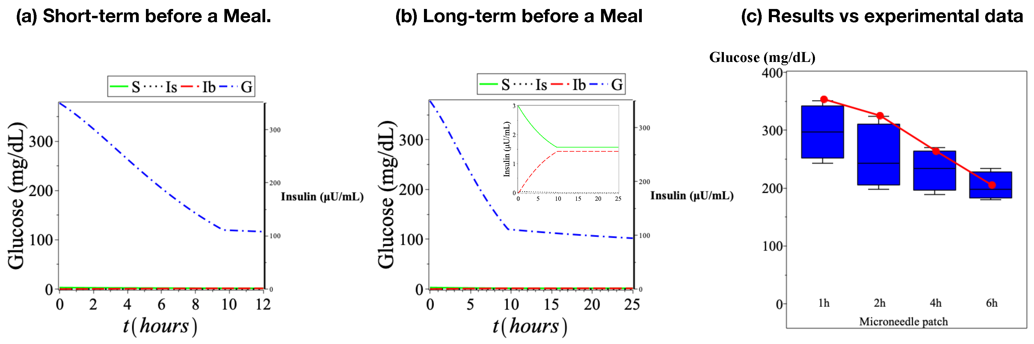
Figure 3. Thesimulation of glucose (mg/dL) and insulin (μU/mL) levels before the meal (Fast) is shown: (a) the short-term behavior over 12 h; (b) the long-term behavior over 24 h; (c) compares the numerically simulated glucose levels (mg/dL) (red curve) with experimental rat data reported in [19] over 6 h. The shaded box represents the experimentally observed blood glucose range.
Mca 31 00041 g003
Figure 4. The simulation of glucose (mg/dL) and insulin (μU/mL) levels after a single meal (20 min) is shown. Panel (a) presents the short-term behavior over 12 h; panel (b) shows the long-term behavior over 24 h; and panel (c) compares the numerically simulated glucose levels (mg/dL) (red curve) with experimental rat data reported in [19] over 6 h. The shaded box represents the experimentally observed blood glucose range.
Mca 31 00041 g004
Figure 5. Simulation of glucose (mg/dL) and insulin (μU/mL) levels after multiple meals (at 5–15 and 22 h): (a) the short-term behavior over 50 h (≈2 days) and (b) the long-term behavior over 100 h (≈4 days).
Mca 31 00041 g005
Table 1. Predicted glucose levels before a meal and after a single meal at selected time points.
Time (h)Before a Meal (mg/dL)After a Single Meal (mg/dL)
1350332
2315308
4260258
6210208
Disclaimer/Publisher’s Note: The statements, opinions and data contained in all publications are solely those of the individual author(s) and contributor(s) and not of MDPI and/or the editor(s). MDPI and/or the editor(s) disclaim responsibility for any injury to people or property resulting from any ideas, methods, instructions or products referred to in the content.