RBF-Based Meshless Collocation Method for Time-Fractional Interface Problems with Highly Discontinuous Coefficients

Abstract

Time-fractional interface problems arise in systems where interacting materials exhibit memory effects or anomalous diffusion. These models provide a more realistic description of physical processes than classical formulations and appear in heat conduction, fluid flow, porous media diffusion, and electromagnetic wave propagation. However, the presence of complex interfaces and the nonlocal nature of fractional derivatives makes their numerical treatment challenging. This article presents a numerical scheme that combines radial basis functions (RBFs) with the finite difference method (FDM) to solve time-fractional partial differential equations involving interfaces. The proposed approach applies to both linear and nonlinear models with constant or variable coefficients. Spatial derivatives are approximated using RBFs, while the Caputo definition is employed for the time-fractional term. First-order time derivatives are discretized using the FDM. Linear systems are solved via Gaussian elimination, and for nonlinear problems, two linearization strategies, a quasi-Newton method and a splitting technique, are implemented to improve efficiency and accuracy. The method’s performance is assessed using maximum absolute and root mean square errors across various grid resolutions. Numerical experiments demonstrate that the scheme effectively resolves sharp gradients and discontinuities while maintaining stability. Overall, the results confirm the robustness, accuracy, and broad applicability of the proposed technique.

1. Introduction

Many physical phenomena occupy domains that are divided into subdomains, each with its own mathematical or physical properties. This leads to the appearance of interfaces, which exist in situations such as fluid flow through heterogeneous materials or structures designed from multiple layers. Propagation of waves through composite materials (a hyperbolic problem) and heat conduction in composite materials (a parabolic problem) are examples related to such interface phenomena. Traditional numerical techniques frequently have difficulty handling interface problems effectively because analytical solutions are rarely available. The main reason is that solutions near interfaces can be discontinuous or not sufficiently smooth, which reduces the accuracy and stability of traditional approaches like the FDM and the finite element method (FEM) [1].

In recent years, researchers in the mathematical and scientific communities have worked intensively to develop improved techniques for solving interface problems. These problems arise across a wide range of fields, including environmental science, biology, materials science, and electromagnetic wave theory [2,3]. Consequently, many numerical methods have been proposed. For example, Babu?ka applied the FDM to solve elliptic interface equations [4]. Aziz et al. developed the Haar wavelet collocation method (HWCM) and meshfree approaches for elliptic and parabolic interface problems [5,6]. Asif and collaborators first applied the HWCM to hyperbolic interface problems and later extended the method to the telegraph equation with interfaces [7,8]. Similarly, Rana and co-authors used the HWCM to solve advection–diffusion–reaction problems involving parabolic and elliptic equations [9]. Ahmad and Islam adopted localized meshless schemes to solve Stokes flow and elliptic interface models [10,11]. Asif and Bilal applied the HWCM to the telegraph equation with discontinuous coefficients [12].

Fractional calculus provides a powerful framework for modeling memory-dependent and anomalous transport phenomena. Over the past decades, fractional differential equations (FDEs) have proven highly effective in describing complex physical processes, including viscoelasticity, rheology, biological systems, dielectric polarization, and turbulent flows [13,14,15,16]. Their ability to capture nonlocal behavior and long-range temporal effects makes fractional operators particularly suitable for problems where classical integer-order models fail to represent the underlying dynamics accurately.

As applications expanded, researchers developed numerous numerical methods for solving FDEs. For example, Zada et al. used the homotopy wavelet collocation method for fractional partial differential equations (FPDEs) [17]. Mehnaz et al. developed a local meshfree method for space-dependent FPDEs [18]. Manzoor and Siraj used a meshless spectral technique to treat the time-fractional Korteweg–de Vries (KdV) equation [19]. Haifa and Carlo employed Chebyshev cardinal functions to approximate time-fractional FPDEs [20]. Rehma and Banan proposed a flexible numerical method for fractional elliptic interface models [21], and Wang et al. applied a space–time FEM to time-fractional diffusion problems with interface conditions [22].

In this work, we focus on one-dimensional time-fractional interface problems where solutions may be discontinuous across interfaces. To solve these problems efficiently and accurately, we employ radial basis functions (RBFs) for spatial discretization in combination with the Caputo derivative for the temporal fractional operator. RBFs offer a meshfree framework and flexible approximation of spatial derivatives, which is particularly advantageous for handling irregular geometries and discontinuities at interfaces [23]. They have been successfully applied in diverse areas, including machine learning, fluid dynamics, biology, image processing, geostatistics, computer graphics, and finance [24]. Comprehensive treatments of RBF theory and practical implementation in MATLAB 7 are provided by Fasshauer [25] and extended by Fasshauer and McCourt [26], while theoretical studies by Franke and Schaback further established convergence and uniqueness properties [27].

In this work, we have focused on one-dimensional (1D) linear and nonlinear time-fractional interface problems, where the interface is fixed. The problem is represented in the following form:

$$D_t^{\rho }\phi (x,t)=\nabla ·(\eta \nabla \phi )+\mathsf{\Phi }, 0<\rho <1, t\ge t_0, \mathrm{in} \mathsf{\Omega },$$

(1)

and

$$D_t^{\rho }\phi (x,t)=\nabla ·(\eta \nabla \phi )+\mathcal{F}(x,t,\phi (x,t))+\mathsf{\Phi }, 0<\rho <1\hspace{1em}t\ge t_0, \mathrm{in} \mathsf{\Omega }.$$

(2)

Let $\phi (x,t)$ be an unknown function, where $\mathcal{F}(x,t,{\phi }_1(x,t))$ represents a nonlinear term. The function $\mathsf{\Phi }(x,t)$ acts as a source term, and $\eta \left(x\right)$ is a smoothly varying coefficient. This formulation is considered for $t\ge t_0$, where $t_0$ denotes the initial time, and $x\in \mathsf{\Omega }$, with $\mathsf{\Omega }\subset \mathbb{R}$ for one-dimensional problems. In this 1D case, the gradient operator reduces to $\nabla =\left({\displaystyle \frac{\partial }{\partial x}}\right)$.

The domain $\mathsf{\Omega }$ is divided into two subdomains by a single interface located at $\theta$. Consequently, the functions $\phi$, a, and $\mathsf{\Phi }$ are defined separately in each subdomain to reflect this partitioning.

$$\begin{array}{c}\hfill (\phi ,a,\mathsf{\Phi })=\left\{\begin{array}{cc}({\phi }^{-},a^{-},{\mathsf{\Phi }}^{-})\hfill & \mathrm{in} {\mathsf{\Omega }}^{-},\hfill \\ ({\phi }^{+},a^{+},{\mathsf{\Phi }}^{+})\hfill & \mathrm{in} {\mathsf{\Omega }}^{+}.\hfill \end{array}\right.\end{array}$$

(3)

The boundary and initial conditions are

$$\begin{array}{cc}\hfill \phi (x,t)& =\chi , (x,t)\in \partial \mathsf{\Omega }\times (0,T_f],\hfill \\ \hfill \phi (x,0)& ={\varpi }_1,\hspace{1em}\mathbf{x}\in \mathsf{\Omega },\hfill \\ \hfill {\phi }_t(x,0)& ={\varpi }_2,\hspace{1em}\mathbf{x}\in \mathsf{\Omega }.\hfill \end{array}$$

(4)

The subsequent interface conditions are imposed at the single interface $x=\theta$:

$$\begin{array}{ccc}\hfill {\left[\phi \right]}_{\theta }& =& {\phi }_1(\theta ,t)-{\phi }_2(\theta ,t)=\omega (\theta ,t),\hfill \end{array}$$

(5)

$$\begin{array}{ccc}\hfill {\left[\eta {\phi }_x\right]}_{\theta }& =& {\eta }^{+}(\theta ,t){\phi }_{1x}(\theta ,t)-{\eta }^{-}(\theta ,t){\phi }_{2x}(\theta ,t)=\nu (\theta ,t).\hfill \end{array}$$

(6)

To simplify the analysis, this paper considers the spatial domain $\mathsf{\Omega }$ as the interval $[0,1]$ for one-dimensional problems. Without loss of generality, the interface is placed at the point $x=\theta$, dividing the domain into two subdomains: ${\mathsf{\Omega }}^{-}=[0,\theta ]$ and ${\mathsf{\Omega }}^{+}=[\theta ,1]$.

To carry out the following analysis, we first introduce some essential definitions and notation related to fractional derivatives.

Definition 1.

The Caputo fractional derivative of order $\rho >0$ for a function $\phi \left(t\right)$, which is absolutely continuous on the interval $[0,T]$, is defined as

$${}^{C}D_t^{\rho }\phi \left(t\right)={\displaystyle \frac{1}{\mathsf{\Gamma }(m-\rho )}}{\int }_0^t{\displaystyle \frac{{\phi }^{\left(m\right)}\left(\zeta \right)}{{(t-\zeta )}^{\rho -m+1}}} d\zeta ,$$

(7)

where $m=\lceil \rho \rceil$ is the smallest integer greater than or equal to ρ, and $\mathsf{\Gamma }(·)$ denotes the Gamma function. This definition extends the concept of a derivative to non-integer (fractional) orders.

This paper is organized like this: In Section 2, we look at radial basis functions. In Section 3, we provide the temporal approximation employing the Caputo derivative for time-fractional interface problems. In Section 4, we talk about spatial discretization. In Section 5, we will discuss stability analysis. Section 6 is for numerical validation. Finally, Section 7 gives some final thoughts and suggests some possible areas for future investigation.

2. Radial Basis Functions

If there is a single-valued function $\psi :[0,\infty )\to \mathbb{R}$ such that $\varphi \left(\mathbf{x}\right)=\psi (\parallel \mathbf{x}\parallel )$, then a function $\varphi :{\mathbb{R}}^d\to \mathbb{R}$ is termed radial. Stated differently, $\varphi \left(\mathbf{x}\right)$ is solely dependent on the magnitude of $\mathbf{x}$ and not on its direction. An RBF is the function $\psi \left(r\right)$, where $r=\parallel \mathbf{x}\parallel$. It is defined with respect to the Euclidean norm for $r\ge 0$.

A positive parameter, known as the shape parameter, is a component of every RBF. The choice of the shape parameter (shown here as $ϵ$), which has a significant impact on the accuracy of the approximation and the conditioning of the final system, is a crucial component of any RBF-based numerical technique. Higher values of $ϵ$ create more peaked bases that are better conditioned but may not be as accurate. On the other hand, lower values create flatter basis functions that may be more accurate but may also lead to ill-conditioned matrices. For this reason, selecting the right form parameter is essential to striking a balance between precision and stability. Numerous research studies have addressed this problem. Cavoretto et al. [28] suggested employing univariate global optimization in conjunction with leave-one-out cross-validation to determine an ideal $ϵ$, showing better results than conventional ad hoc selections. More recently, Cavoretto et al. [29] presented a Bayesian optimization strategy for choosing the form parameter in RBF methods, emphasizing its influence on robustness and accuracy. Based on these findings, $ϵ$ is selected in the current work to guarantee a dependable and effective approximation. In this work, we employ the multiquadric radial basis function (MQ-RBF) because extensive analytical and numerical studies have shown that MQ offers higher approximation accuracy, smoother derivative reproduction, and better stability for PDE collocation compared with Gaussian, inverse multiquadric (IMQ), or thin-plate spline (TPS) kernels. MQ-RBF is one of the most popular RBFs and was first used in the interpolation method by Hardy [30]. Interpolation by using polynomials and trigonometric functions is popular but deficient in some aspects. The MQ interpolation scheme was unnoticed until 1979, but the method received much attention when Richard Franked concluded that the MQ RBF interpolation is the best among various interpolation methods to solve the scattered data interpolation problem [31]. The popularity of the method increased further when Edward Kansa [32] solved PDEs through the MQ-RBF method. An advantage of MQ-RBF is its low computational cost and high accuracy even for small shape parameters, making it especially effective for stable derivative evaluation in interface problems. The following is the mathematical form of MQ-RBFs:

$$\varphi \left(r\right)=\sqrt{1+{\left(ϵr\right)}^2},$$

where r = $\left|\right|x-x_i\left|\right|$, and x is the center point [33].

RBFs are typically used for the approximation defined on scattered data of the form

$$\phi (x,t)=\sum _{i=1}^{\mathcal{N}}{\lambda }_i\varphi \left(\right||x-x_i\left|\right|),$$

(8)

where $\phi (x,t)$ is an approximated function whose value depends upon the sum of $\mathcal{N}$ radial basis functions. Each basis function depends upon different weights ${\lambda }_i$ and centers $x_i$. The weight can be calculated by simplifying the linear equations. Let ${\phi }_i=\phi \left(x_i\right)$; the weight ${\lambda }_i$ can be solved by

$$\left[\begin{array}{ccc}{\varphi }_{1,1}& \dots & {\varphi }_{1,F}\\ ⋮& ⋮& ⋮\\ {\varphi }_{F,1}& \dots & {\varphi }_{F,F}\end{array}\right]\left[\begin{array}{c}{\alpha }_1\\ ⋮\\ {\alpha }_e\end{array}\right]=\left[\begin{array}{c}{\beta }_1\\ ⋮\\ {\beta }_m\end{array}\right]$$

(9)

Advantages and Disadvantages of the Meshless Collocation Method (MCM)

The MCM with RBFs has been extensively applied to compute numerical solutions for a broad spectrum of ODEs and PDEs. This method offers several significant advantages:

• The method is efficient, capable of delivering accurate results using only a limited number of nodes.
• The method is well-suited for PDE problems involving complicated and non-uniform domains.
• The method maintains manageable computational requirements as the dimensionality increases.
• There is no need to define nodal or element connectivity.
• Unlike many other numerical techniques, this method does not require numerical integration.

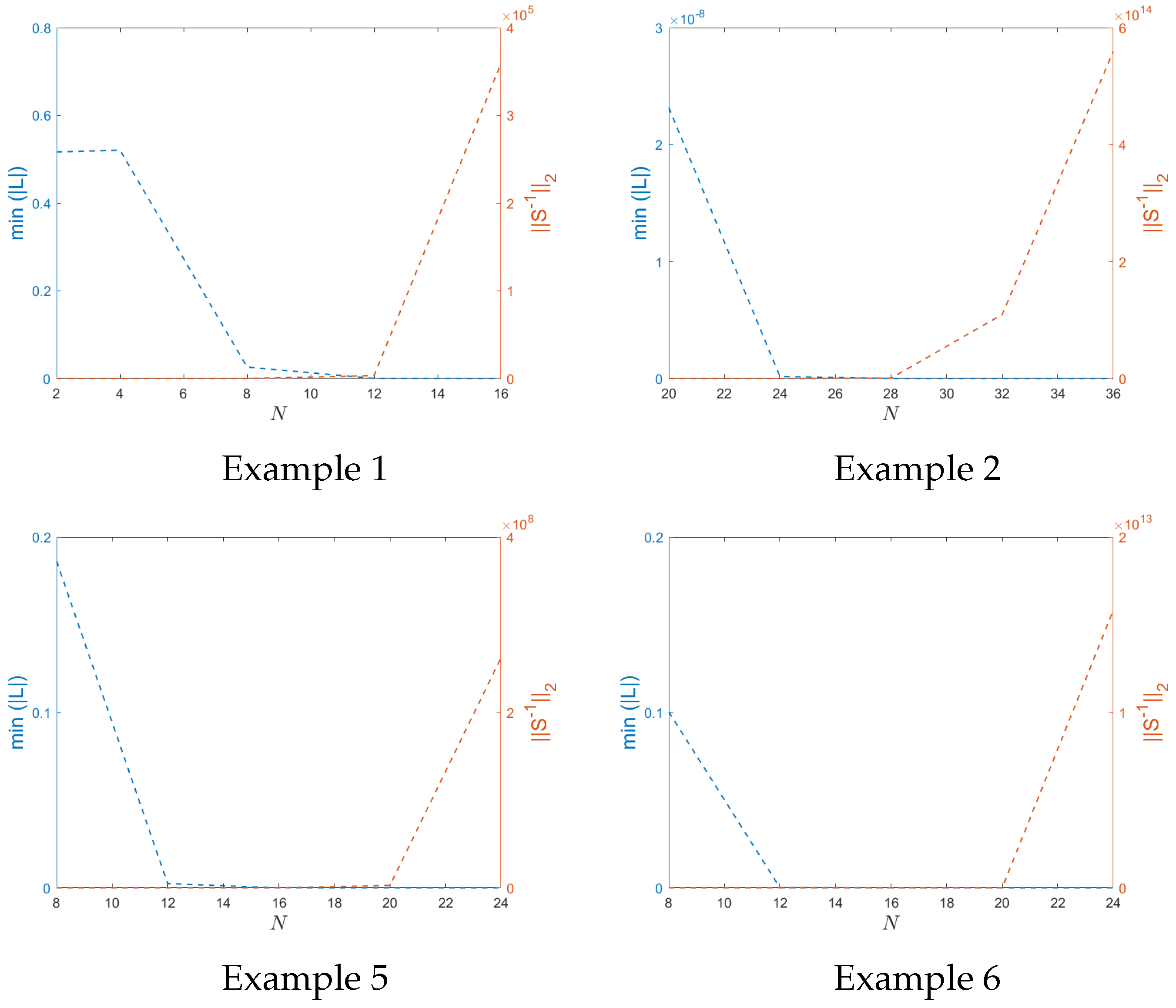
However, like any numerical method, the MCM also has some drawbacks. One limitation of applying the MCM with RBFs is the tendency for the discretized system matrices to exhibit ill-conditioning. To address this issue, regularization techniques such as truncated singular value decomposition are often employed to improve the stability of the solution.

3. Temporal Approximation Using Caputo Derivative

This section aims to derive the Caputo fractional derivative for $\rho \in (0,1)$, which is defined by

$${\displaystyle \frac{{\partial }^{\rho }\phi }{\partial t^{\rho }}}=\left\{\begin{array}{cc}{\displaystyle \frac{1}{\mathsf{\Gamma }\left(1-\rho \right)}}\underset{0}{\overset{t}{\int }}{\phi }^{\prime }\left(t\right){\left(t-\zeta \right)}^{-\rho }d\zeta ,\hfill & 0<\rho <1.\hfill \\ \hfill & \\ {\displaystyle \frac{\partial \phi }{\partial t}},\hfill & \rho =1.\hfill \end{array}\right.$$

Differentiating at $t=t^{m+1}$, we obtain

$${\displaystyle \frac{{\partial }^{\rho }\phi (\phi ,t^{m+1})}{\partial t^{\rho }}}={\displaystyle \frac{1}{\mathsf{\Gamma }(1-\rho )}}\underset{0}{\overset{t^{m+1}}{\int }}{\phi }^{\prime }\left(\zeta \right){\left(t^{m+1}-\zeta \right)}^{-\rho }d\zeta ,$$

$$\Rightarrow {\displaystyle \frac{{\partial }^{\rho }\phi )}{\partial t^{\rho }}}={\displaystyle \frac{1}{\mathsf{\Gamma }(1-\rho )}}\sum _{k=0}^m\underset{t^k}{\overset{t^{k+1}}{\int }}{\phi }^{\prime }\left(t\right){\left(t^{m+1}-\zeta \right)}^{-\rho }d\zeta$$

Now, we apply the FDM to approximate ${\displaystyle \frac{{\partial }^{m+1}\phi }{\partial t^{m+1}}}$, as follows:

$${\displaystyle \frac{\partial \phi (\phi ,{\zeta }^{k+1})}{\partial \zeta }}={\displaystyle \frac{{\phi }^{k+1}-{\phi }^k}{dt}}+o\left(dt\right).$$

Then

$${\displaystyle \frac{{\partial }^{\rho }\phi (\phi ,t^{m+1})}{\partial t^{\rho }}}\approx {\displaystyle \frac{1}{\mathsf{\Gamma }(1-\rho )}}\sum _{k=0}^m\underset{t^k}{\overset{t^{k+1}}{\int }}{\displaystyle \frac{{\phi }^{k+1}-{\phi }^k}{dt}}{\left(t^{m+1}-\zeta \right)}^{-\rho }d\zeta ,$$

$${\displaystyle \frac{{\partial }^{\rho }\phi }{\partial t^{\rho }}}=a_0\sum _{k=0}^m{b}_k\left(u^{m-k+1}-{\phi }^{m-k}\right),$$

where $b_k={(k+1)}^{1-\rho }-k^{1-\rho }$, $k=0,1,\dots ,m$ and $a_0={\displaystyle \frac{d{t}^{-\rho }}{\mathsf{\Gamma }(2-\rho )}}$.

Finally, we can express it in a more refined form as follows:

$${\displaystyle \frac{{\partial }^{\rho }\phi }{\partial t^{\rho }}}=\left\{\begin{array}{cc} \hfill & \\ a_0\left({\phi }^{m+1}-{\phi }^m\right)+a_0{\displaystyle \sum _{k=1}^m}{b}_k\left({\phi }^{m-k+1}-{\phi }^{m-k}\right),\hfill & n\ge 1,\hfill \\ \hfill & \\ a_0\left({\phi }^1-{\phi }^0\right),\hfill & m=0.\hfill \end{array}\right.$$

(10)

4. Meshless Collocation Approach for Single Interface Model

The interval $[0,1]$ is split into two subintervals: ${\mathsf{\Omega }}^{+}=[0,\theta ]$ and ${\mathsf{\Omega }}^{-}=[\theta ,1]$. The first subinterval ${\mathsf{\Omega }}^{+}$ is discretized using nodes such that $0=x_1<x_2<\cdots <x_{{\mathcal{M}}_1+1}=\alpha$. Similarly, the second subinterval ${\mathsf{\Omega }}^{-}$ is discretized as $x_{{\mathcal{M}}_1+1}=\alpha <x_{{\mathcal{M}}_1+2}<\cdots <x_{\mathcal{N}}=1$, where $\mathcal{N}={\mathcal{M}}_1+{\mathcal{M}}_2+1$ represents the total number of nodes, and ${\mathcal{M}}_1$ and ${\mathcal{M}}_2$ denote the number of divisions in ${\mathsf{\Omega }}^{+}$ and ${\mathsf{\Omega }}^{-}$, respectively. The estimation of the function ${\phi }_1(x,t)$ on the interval ${\mathsf{\Omega }}^{+}$ using the multiquadric MQ-RBF is expressed as follows.

On the interval $I=[0,\alpha )$, we approximate ${\phi }_1(x,t)$ by employing MQ-RBFs in the following manner:

$${\phi }_1(x,t)=\sum _{i=1}^{\mathcal{M}+1}{\lambda }_i \varphi (\parallel x-x_i\parallel ), x\in {\mathsf{\Omega }}^{+},$$

(11)

where ${\mathsf{\Omega }}^{+}=[0,\theta )$, and $\varphi$ is the MQ radial basis function.

Differentiating Equation (11) with respect to x, we obtain

$${\phi }_{1x}(x,t)=\sum _{i=1}^{\mathcal{M}+1}{\lambda }_i {\displaystyle \frac{d\varphi }{dx}}(\parallel x-x_i\parallel ), x\in {\mathsf{\Omega }}^{+},$$

(12)

and the second derivative is given by

$${\phi }_{1xx}(x,t)=\sum _{i=1}^{\mathcal{M}+1}{\lambda }_i {\displaystyle \frac{d^2\varphi }{d{x}^2}}(\parallel x-x_i\parallel ), x\in {\mathsf{\Omega }}^{+}.$$

(13)

Similarly, the unknown function ${\phi }_2(x,t)$ is approximated over the interval ${\mathsf{\Omega }}^{-}=[\theta ,1]$ as

$${\phi }_2(x,t)=\sum _{i=\mathcal{M}+1}^{\mathcal{N}}{\gamma }_i \varphi (\parallel x-x_i\parallel ), x\in {\mathsf{\Omega }}^{-}.$$

(14)

Differentiating Equation (14) with respect to x yields

$${\phi }_{2x}(x,t)=\sum _{i=\mathcal{M}+1}^{\mathcal{N}}{\gamma }_i {\displaystyle \frac{d\varphi }{dx}}(\parallel x-x_i\parallel ), x\in {\mathsf{\Omega }}^{-},$$

(15)

and the second derivative becomes

$${\phi }_{2xx}(x,t)=\sum _{i=\mathcal{M}+1}^{\mathcal{N}}{\gamma }_i {\displaystyle \frac{d^2\varphi }{d{x}^2}}(\parallel x-x_i\parallel ), x\in {\mathsf{\Omega }}^{-}.$$

(16)

Approximating the boundary conditions at $x=0$ and $x=1$ using Equations (11) and (14), we obtain

$$\begin{array}{cc}\hfill \sum _{i=1}^{\mathcal{M}+1}{\lambda }_i \varphi (\parallel 0-x_i\parallel )& ={\mathsf{\Theta }}_1\left(t\right),\hfill \end{array}$$

(17)

$$\begin{array}{cc}\hfill \sum _{i=\mathcal{M}+1}^{\mathcal{N}}{\gamma }_i \varphi (\parallel 1-x_i\parallel )& ={\mathsf{\Theta }}_2\left(t\right),\hfill \end{array}$$

(18)

where ${\mathsf{\Theta }}_1\left(t\right)=\phi (0,t)$ and ${\mathsf{\Theta }}_2\left(t\right)=\phi (1,t)$. The meshless approximations for the interface conditions are given by

$$\sum _{i=1}^{\mathcal{M}+1}{\lambda }_i \varphi (\parallel x-x_i\parallel )-\sum _{i=\mathcal{M}+1}^{\mathcal{N}}{\gamma }_i \varphi (\parallel x-x_i\parallel )=q_1\left(t\right),$$

(19)

$${\eta }^{+}\left(\sum _{i=1}^{\mathcal{M}+1}{\lambda }_i {\displaystyle \frac{d\varphi }{dx}}(\parallel x-x_i\parallel )\right)-{\eta }^{-}\left(\sum _{i=\mathcal{M}+1}^{\mathcal{N}}{\gamma }_i {\displaystyle \frac{d\varphi }{dx}}(\parallel x-x_i\parallel )\right)=q_2\left(t\right).$$

(20)

We will solve the above system for both linear and nonlinear cases separately.

4.1. Linear Case

For the linear time-fractional interface problems described in Equation (1), we obtain

$$\begin{array}{ccc}& & a_0\left(\sum _{i=1}^{\mathcal{M}+1}{\lambda }_i \varphi (\parallel x-x_i\parallel )-{\phi }_1(x,t_0)+\sum _{k=0}^m{b}_k({\phi }^{m-k+1}-{\phi }^{m-k})\right)={\eta }_x^{+}\left(x\right)\sum _{i=1}^{\mathcal{M}+1}{\lambda }_i {\displaystyle \frac{d\varphi }{dx}}(\parallel x-x_i\parallel )\hfill \\ & & +{\eta }^{+}\left(x\right)\sum _{i=1}^{\mathcal{M}+1}{\lambda }_i {\displaystyle \frac{d^2\varphi }{d{x}^2}}(\parallel x-x_i\parallel )+f_1(x,t), x\in {\mathsf{\Omega }}^{+}.\hfill \end{array}$$

(21)

and

$$\begin{array}{ccc}& & a_0\left(\sum _{i=\mathcal{M}+1}^{\mathcal{N}}{\gamma }_i \varphi (\parallel x-x_i\parallel )-{\phi }_2(x,t_0)+\sum _{k=0}^m{b}_k({\phi }^{m-k+1}-{\phi }^{m-k})\right)={\eta }_x^{-}\left(x\right)\sum _{i=\mathcal{M}+1}^{\mathcal{N}}{\gamma }_i {\displaystyle \frac{d\varphi }{dx}}(\parallel x-x_i\parallel )\hfill \\ & & +{\eta }^{-}\left(x\right)\sum _{i=\mathcal{M}+1}^{\mathcal{N}}{\gamma }_i {\displaystyle \frac{d^2\varphi }{d{x}^2}}(\parallel x-x_i\parallel )+f_2(x,t), x\in {\mathsf{\Omega }}^{-}.\hfill \end{array}$$

(22)

Now, discretizing the following equation, we have

$$\begin{array}{ccc}\hfill & & a_0\left(\sum _{i=1}^{\mathcal{M}+1}{\lambda }_i \varphi (\parallel x_j-x_i\parallel )\right)-{\eta }_x^{+}\left(x\right)\sum _{i=1}^{\mathcal{M}+1}{\lambda }_i {\displaystyle \frac{d\varphi }{dx}}(\parallel x_j-x_i\parallel )-{\eta }^{+}\left(x\right)\sum _{i=1}^{\mathcal{M}+1}{\lambda }_i {\displaystyle \frac{d^2\varphi }{d{x}^2}}(\parallel x_j-x_i\parallel )\hfill \\ & & ={\phi }_1(x_j,t_0)-a_0\sum _{k=0}^m{b}_k({\phi }^{m-k+1}-{\phi }^{m-k})+f_1(x,t), x\in {\mathsf{\Omega }}^{+}.\hfill \end{array}$$

(23)

and

$$\begin{array}{ccc}\hfill & & a_0\left(\sum _{i=\mathcal{M}+1}^{\mathcal{N}}{\gamma }_i \varphi (\parallel x_j-x_i\parallel )\right)-{\eta }_x^{-}\left(x\right)\sum _{i=\mathcal{M}+1}^{\mathcal{N}}{\gamma }_i {\displaystyle \frac{d\varphi }{dx}}(\parallel x_j-x_i\parallel )-{\eta }^{-}\left(x\right)\sum _{i=\mathcal{M}+1}^{\mathcal{N}}{\gamma }_i {\displaystyle \frac{d^2\varphi }{d{x}^2}}(\parallel x_j-x_i\parallel )\hfill \\ & & ={\phi }_2(x_j,t_0)-\sum _{k=0}^m{b}_k({\phi }^{m-k+1}-{\phi }^{m-k})+f_2(x,t), x\in {\mathsf{\Omega }}^{-}.\hfill \end{array}$$

(24)

A linear system consisting of $\mathcal{N}+1$ unknowns is formulated using Equations (19), (20), (23), and (24). In this system, the functions ${\lambda }_i\left(\tau \right)$ for $i=1,2,\dots ,\mathcal{M}+1$ and ${\gamma }_i\left(\tau \right)$ for $i=\mathcal{M}+1,\mathcal{M}+2,\dots ,\mathcal{N}$ appear as key components in the expression.

4.2. Nonlinear Case

4.2.1. Quasi-Newton Linearization Technique

The first step in addressing the nonlinear case involves applying the quasi-Newton linearization formula to Equation (2).

$${\left(\nu \mu \right)}^{m+1}={\nu }^m{\mu }^{m+1}+{\nu }^{m+1}{\mu }^m-{\nu }^m{\mu }^m+\mathcal{O}(\Delta {\mathtt{t}}^2).$$

(25)

The theoretical foundation and rigorous proof of the proposed approach are presented in [34].

An analogous method can be adopted to handle nonlinear time-fractional interface problems.

4.2.2. Innovative Splitting Technique

The governing equation under consideration is a nonlinear time-fractional partial differential equation:

$$D_{\mathtt{t}}^{\rho }\phi (\mathtt{x},\mathtt{t})-\nabla ·(\eta \nabla \phi )=\mathcal{F}(\mathtt{x},\mathtt{t},\phi (\mathtt{x},\mathtt{t})), 0<\rho <1, \mathtt{t}>0, \mathtt{x}\in \mathsf{\Omega },$$

(26)

where $D_{\mathtt{t}}^{\rho }$ denotes the fractional derivative of order $\rho$, and $\mathcal{F}$ is a nonlinear function of the solution $\phi$. To handle the nonlinearity, we reformulate the source term. The nonlinear operator $\mathcal{N}\left(\phi \right)$ is defined as

$$\mathcal{N}\left(\phi \right)={\displaystyle \frac{\mathcal{F}(\mathtt{x},\mathtt{t},\phi )}{\phi }},$$

(27)

provided that $\phi \ne 0$ in the domain. This allows the original equation to be rewritten as

$$D_{\mathtt{t}}^{\rho }\phi (\mathtt{x},\mathtt{t})-\nabla ·(\eta \nabla \phi )+\mathcal{N}\left(\phi \right)\phi =f(\mathtt{x},\mathtt{t}).$$

(28)

In this form, $\mathcal{N}\left(\phi \right)\phi$ constitutes the nonlinear term.

To ensure the numerical solution remains positive, thereby guaranteeing that $\mathcal{N}\left(\phi \right)$ is well-defined, we apply the transformation

$$\phi (\mathtt{x},\mathtt{t})=v(\mathtt{x},\mathtt{t})+c,$$

(29)

where c is a sufficiently large positive constant chosen such that $\phi >0$ throughout the computational domain $\mathsf{\Omega }$. Substituting this into the equation and noting that $\nabla \phi =\nabla v$ and $D_{\mathtt{t}}^{\rho }\phi =D_{\mathtt{t}}^{\rho }v$, the transformed equation for v is

$$D_{\mathtt{t}}^{\rho }v(\mathtt{x},\mathtt{t})-\nabla ·(\eta \nabla v)+\mathcal{N}(v+c)(v+c)=f(\mathtt{x},\mathtt{t}).$$

(30)

The corresponding Dirichlet boundary condition becomes

$$v(\mathtt{x},\mathtt{t})=\mu (\mathtt{x},\mathtt{t}), \mathtt{x}\in \partial \mathsf{\Omega },$$

(31)

where $\mu (\mathtt{x},\mathtt{t})$ is the prescribed boundary data. For the sake of notational simplicity in the subsequent linearization process, we will continue to use $\phi$ with the understanding that it now represents the positively shifted solution $v+c$.

Linearization Process

The nonlinear term $\mathcal{N}\left(\phi \right)\phi$ is linearized using a relaxation splitting technique, splitting the term as

$$\mathcal{N}\left(\phi \right)\phi =\omega \mathcal{N}\left(\phi \right)\phi +(1-\omega )\mathcal{N}\left(\phi \right)\phi ,$$

(32)

where $\omega \in [0,1]$ is a relaxation parameter. In an iterative solution process (denoting the current iteration as $k+1$ and the previous known iteration as k), we treat part of the term explicitly. Specifically, the term multiplied by $\omega$ is evaluated at the previous iteration ${\phi }^k$ and moved to the right-hand side as a source term. The term multiplied by $(1-\omega )$ is kept on the left-hand side and evaluated at the current unknown ${\phi }^{k+1}$. This yields the following linearized equation for the next iterative solution ${\phi }^{k+1}$:

$$D_{\mathtt{t}}^{\rho }{\phi }^{k+1}(\mathtt{x},\mathtt{t})-\nabla ·(\eta \nabla {\phi }^{k+1})+(1-\omega )\mathcal{N}\left({\phi }^{k+1}\right){\phi }^{k+1}=f(\mathtt{x},\mathtt{t})+\omega \mathcal{N}\left({\phi }^k\right){\phi }^k, \mathtt{x}\in \mathsf{\Omega }.$$

(33)

The relaxation parameter $\omega$ plays a critical role in controlling how much the previous iteration contributes to the current update, thereby ensuring a balanced and stable convergence process. In our numerical experiments, its value was selected empirically. We tested several candidate values of $\omega$ and evaluated their corresponding errors, as reported in Table 7, and then fixed the value that provided the best balance between convergence rate and stability for the considered problem configurations. More advanced strategies, such as adaptive line search techniques, may further improve efficiency [35,36].

A similar scheme can also be extended to nonlinear time-fractional interface problems.

5. Stability Analysis

We analyze the stability of the established MQ-RBFs following the basic definition described in LeVeque’s work on numerical schemes [37].

Definition 2.

In the numerical solution of the interface problem, the resulting system $\mathbf{X}a=b$ is considered stable if the matrix $\mathbf{X}$ has a bounded inverse:

$$\parallel {\mathbf{X}}^{-1}\parallel \le l_0,$$

where $l_0$ is a constant. The stability trend of the scheme is shown in Figure 1.

6. Numerical Validation

To assess the performance of the proposed MQ-RBF, numerical solutions for time-fractional interface problems are obtained, and their accuracy is determined via the following error norms:

$$\begin{array}{ccc}\hfill MAEs& =& \left|\right|{\phi }^{true}-{\phi }^{approx}{\left|\right|}_{\infty }\approx max\left(\right|{\phi }_j^{true}-{\phi }_j^{approx}\left|\right),\hfill \end{array}$$

(34)

$$\begin{array}{ccc}\hfill RMSEs& \approx & \sqrt{\left({\displaystyle \frac{1}{M}}\sum _{j=1}^M{({\phi }_j^{true}-{\phi }_j^{approx})}^2\right)}.\hfill \end{array}$$

(35)

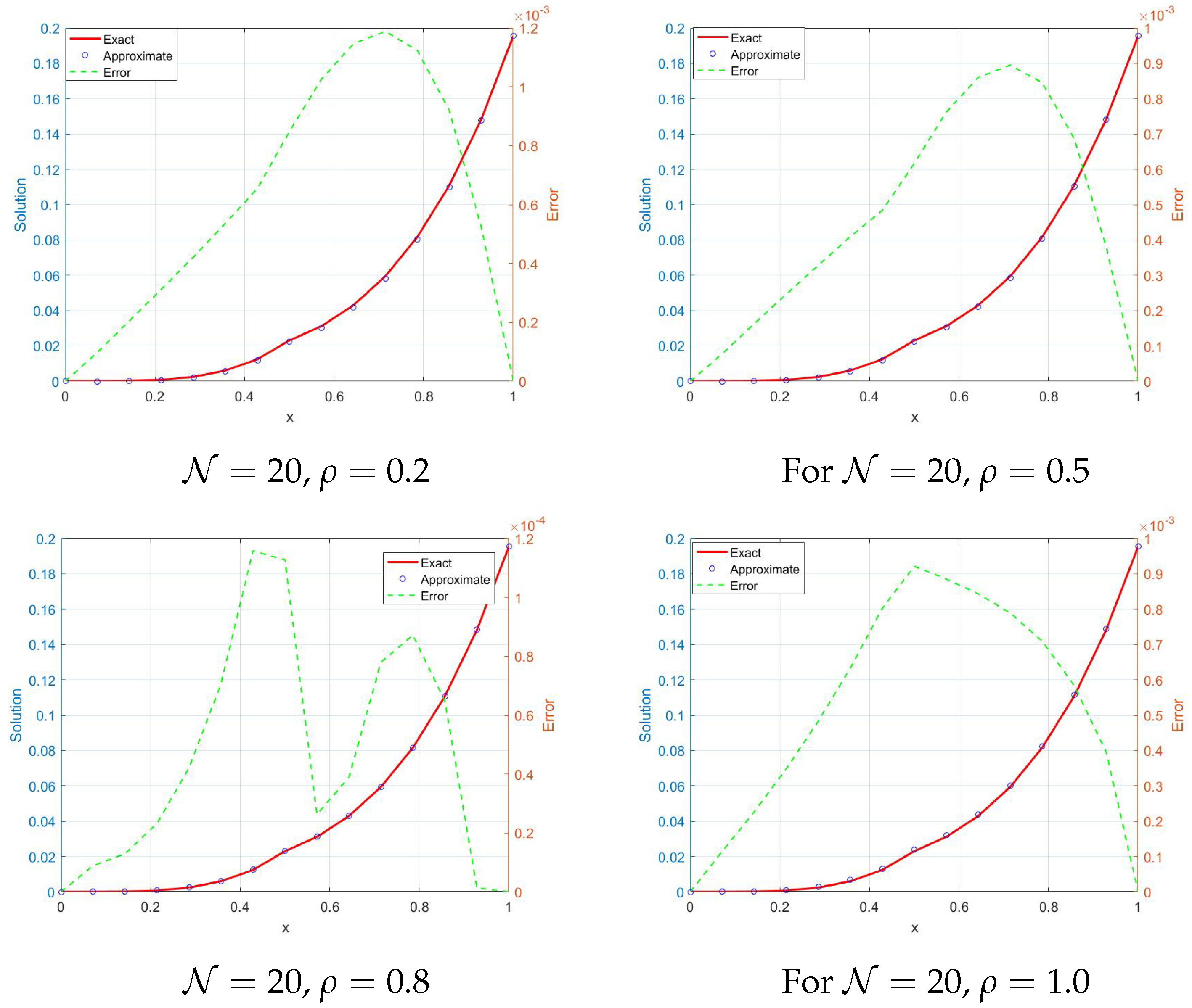
Example 1.

As the first example, linear time-fractional interface Problem (1) is considered assuming ${\eta }^{+}\left(x\right)=1$ and ${\eta }^{-}\left(x\right)=2$. Exact solutions and source functions are given by

$$\phi (x,t)=\left\{\begin{array}{cc}{\phi }_1(x,t)=x^8{e}^{-t},\hfill & 0\le x\le {\displaystyle \frac{1}{2}},\hfill \\ {\phi }_2(x,t)={\displaystyle \frac{1}{2}}\left(x^8+{\displaystyle \frac{1}{256}}\right)e^{-t},\hfill & {\displaystyle \frac{1}{2}}\le x\le 1,\hfill \end{array}\right.$$

(36)

and

$$f(x,t)=\left\{\begin{array}{cc}{f}_1(x,t)=-56x^6{e}^{-t}-t^{1-\rho }{\mathcal{M}}_{1,2-\rho }(-t)x^8,\hfill & 0\le x\le {\displaystyle \frac{1}{2}},\hfill \\ f_2(x,t)=-{\displaystyle \frac{1}{2}}{t}^{1-\rho }{\mathcal{M}}_{1,2-\rho }(-t)(x^8+{\displaystyle \frac{1}{256}})-56x^6{e}^{-t}{e}^{-t},\hfill & {\displaystyle \frac{1}{2}}\le x\le 1.\hfill \end{array}\right.$$

(37)

where ${\mathcal{M}}_{a,b}(·)$ is the Mittag–Leffler function of two parameters defined as

$${\mathcal{M}}_{a,b}\left(t\right)=\sum _{k=0}^{\infty }{\displaystyle \frac{t^k}{\mathsf{\Gamma }(ak+b)}}, \forall t\in \mathbb{C}, a,b\in {\mathbb{R}}^{+}$$

and

$${\mathcal{M}}_{1,1}\left(t\right)=exp\left(t\right), \forall t\in \mathbb{C}.$$

For this linear 1D time-fractional interface problem, the true solution calculates the interface, boundary, and initial conditions. The MQ-RBF method is applied to approximate the solution, and the corresponding numerical results are summarized in

Table 1. Error analysis for different values of $\rho$ and N with $ϵ=2$, $dt=0.5$, and $t=1$ for Example 1 using Caputo derivative.

$\mathcal{N}$	$\mathsf{\rho }=0.2$		$\mathsf{\rho }=0.5$		$\mathsf{\rho }=0.8$		$\mathsf{\rho }=1$
	MAEs	RMSEs	MAEs	RMSEs	MAEs	RMSEs	MAEs	RMSEs
4	1.9357 × 10−2	1.0229 × 10−2	1.9435 × 10−2	1.0249 × 10−2	1.9605 × 10−2	1.0261 × 10−2	1.9769 × 10−2	1.0260 × 10−2
8	1.1877 × 10−2	6.9440 × 10−3	1.2080 × 10−2	7.0897 × 10−3	1.2124 × 10−2	7.1383 × 10−3	1.2023 × 10−2	7.0880 × 10−3
12	4.6615 × 10−3	2.7498 × 10−3	4.6907 × 10−3	2.7712 × 10−3	4.5710 × 10−3	2.6904 × 10−3	4.3842 × 10−3	2.5660 × 10−3
16	1.7356 × 10−3	1.0803 × 10−3	1.6864 × 10−3	1.0395 × 10−3	1.4945 × 10−3	8.9482 × 10−4	1.2721 × 10−3	7.3903 × 10−4
20	8.2722 × 10−4	5.7592 × 10−4	7.5320 × 10−4	5.1184 × 10−4	5.3881 × 10−4	3.3914 × 10−4	3.0553 × 10−4	1.7841 × 10−4
24	6.1504 × 10−4	4.4172 × 10−4	5.1052 × 10−4	3.7034 × 10−4	2.7253 × 10−4	1.8611 × 10−4	1.2150 × 10−4	6.0137 × 10−5

. The tests conducted for different fractional orders $\rho$ and collocation points $\mathcal{N}$ demonstrate, through MAE and RMSE metrics, that the technique achieves high precision. As $\mathcal{N}$ increases, the errors decrease consistently. For example, when $\mathcal{N}=24$, the MAEs are $6.1504\times {10}^{-4}$ for $\rho =0.2$ and $1.2150\times {10}^{-4}$ for $\rho =1$. These results indicate that the accuracy improves as $\rho$ approaches the classical case of integer order. The method remains stable and convergent in all the values tested in $\rho$, although smaller fractional orders tend to produce slightly larger errors due to the stronger memory effects inherent in fractional models. To further illustrate the behavior of the solution, a surface plot 3D for $\rho =0.5$ is provided in Figure 2. Additionally, Figure 3 compares the solution profiles for several values of $\rho$, providing further insight into how fractional order influences system dynamics.

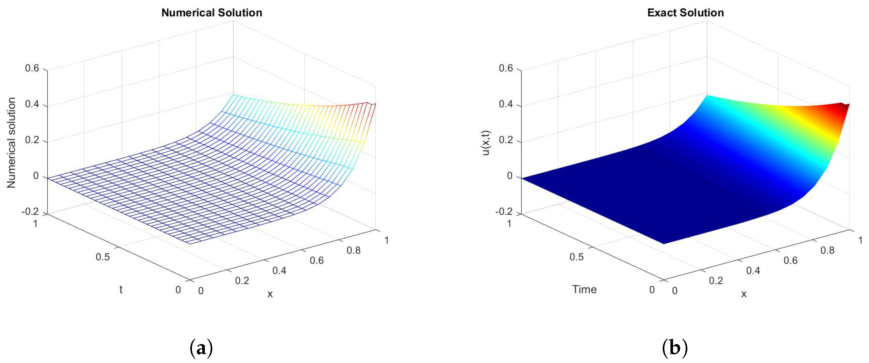
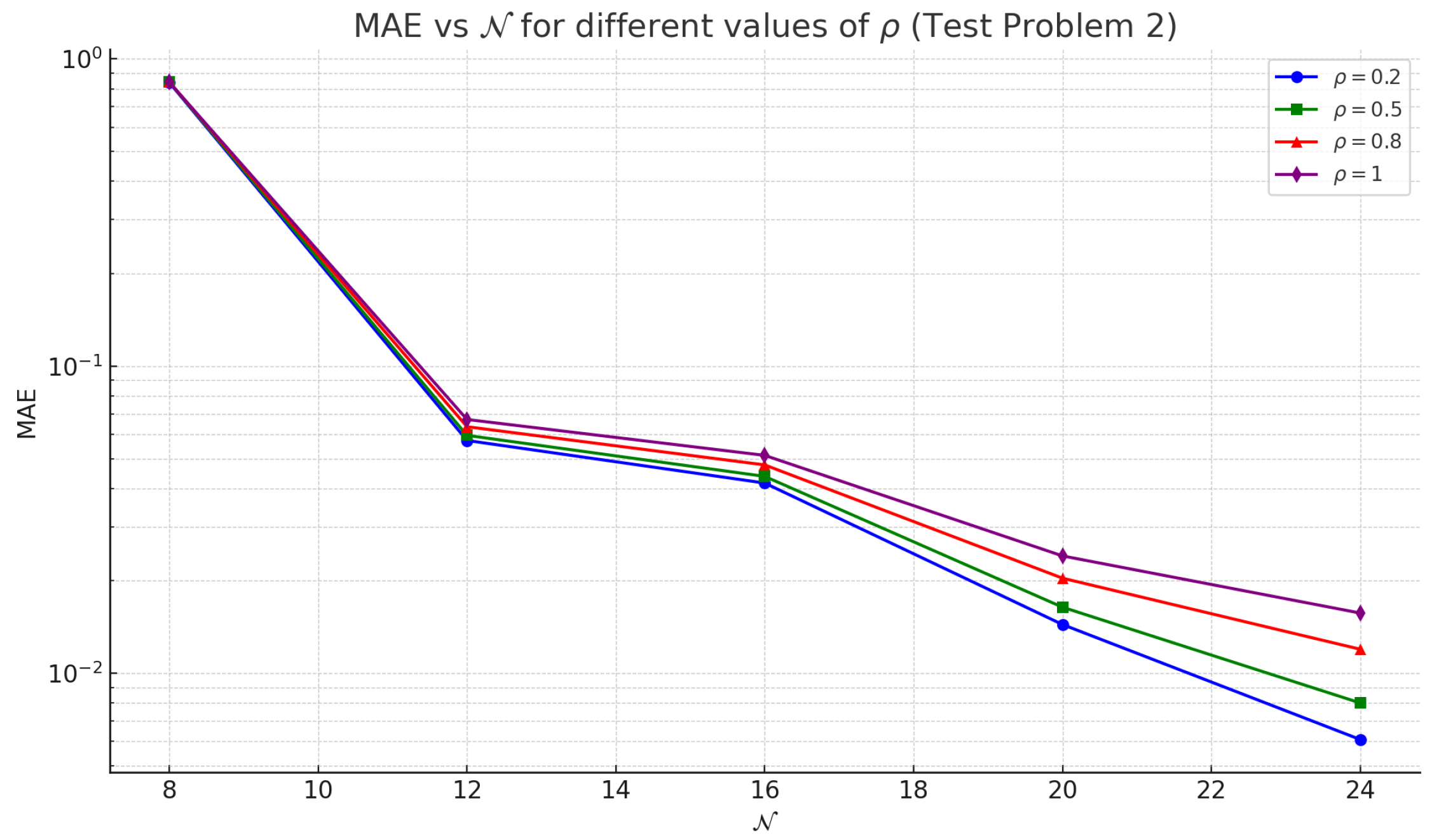
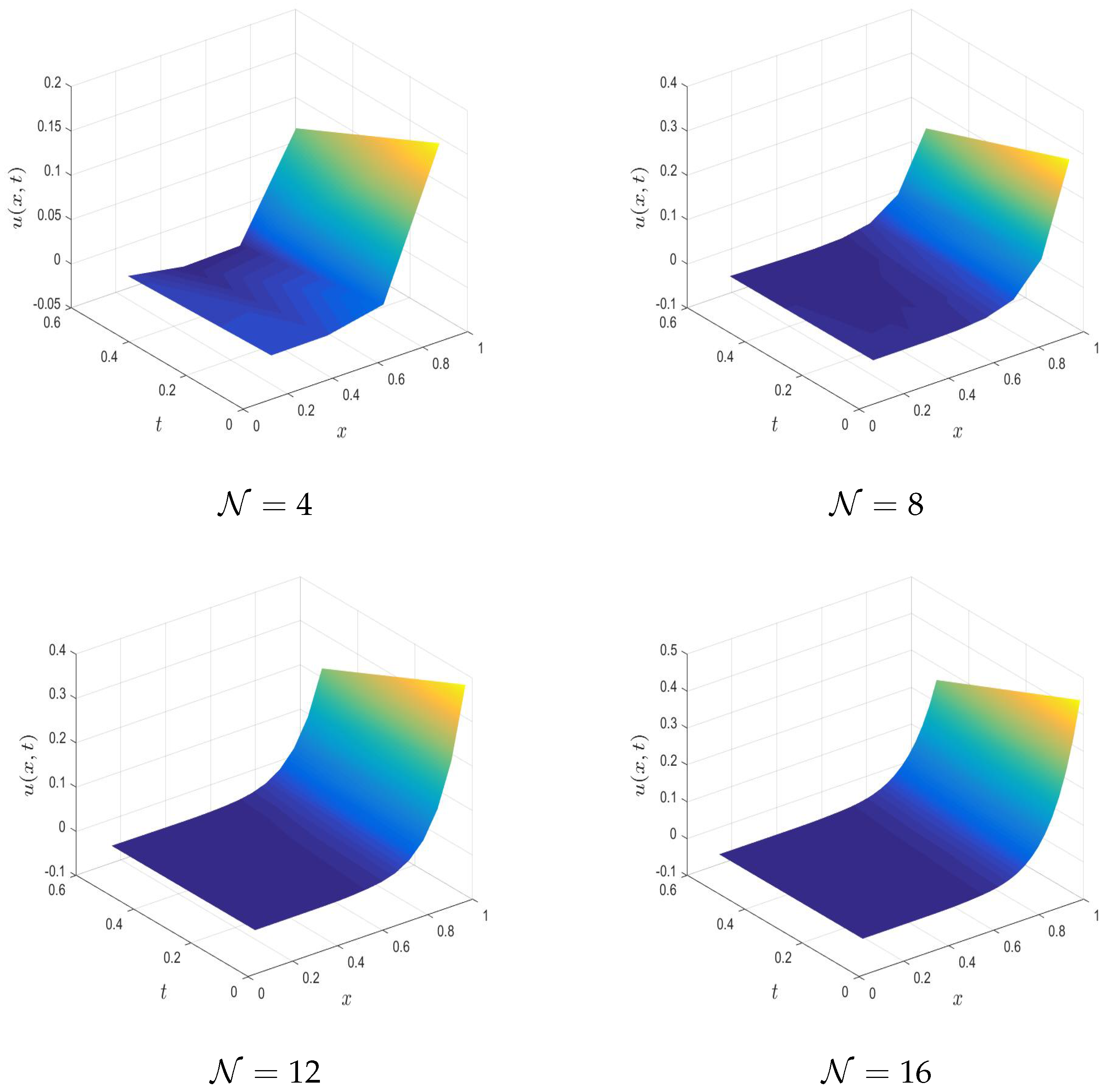
Example 2.

As the second example, linear time-fractional interface Problem (1) is considered assuming ${\eta }^{+}\left(x\right)=exp(-10{(x-0.5)}^4{x}^4)$ and ${\eta }^{-}\left(x\right)=3$. Exact solutions and source functions are given by

$$\phi (x,t)=\left\{\begin{array}{cc}{\phi }_1(x,t)=sin5\pi x{e}^{-t},\hfill & 0\le x\le {\displaystyle \frac{1}{2}},\hfill \\ {\phi }_2(x,t)=(2{(x-{\displaystyle \frac{1}{2}})}^7+1)e^{-t},\hfill & {\displaystyle \frac{1}{2}}\le x\le 1,\hfill \end{array}\right.$$

(38)

and

$$f(x,t)=\left\{\begin{array}{c}{f}_1(x,t)=-t^{1-\rho }{\mathcal{M}}_{1,2-\rho }(-t)sin\left(5\pi x\right)+15\pi e^{-t-10x^4{(x-{\displaystyle \frac{1}{2}})}^4}cos\left(5\pi x\right)(40x^3{(x-{\displaystyle \frac{1}{2}})}^4\hfill \\ +40x^4{(t-{\displaystyle \frac{1}{2}})}^3),\hfill & 0\le x\le {\displaystyle \frac{1}{2}},\hfill \\ f_2(x,t)=-t^{1-\rho }{\mathcal{M}}_{1,2-\rho }(-t)\left(2{(x-{\displaystyle \frac{1}{2}})}^7+1\right)\hfill \\ -252exp(-t){(x-{\displaystyle \frac{1}{2}})}^5,\hfill & {\displaystyle \frac{1}{2}}\le x\le 1.\hfill \end{array}\right.$$

(39)

where ${\mathcal{M}}_{a,b}(·)$ is the Mittag–Leffler function of two parameters defined as

$${\mathcal{M}}_{a,b}\left(t\right)=\sum _{k=0}^{\infty }{\displaystyle \frac{t^k}{\mathsf{\Gamma }(ak+b)}}, \forall t\in \mathbb{C}, a,b\in {\mathbb{R}}^{+}$$

and

$${\mathcal{M}}_{1,1}\left(t\right)=exp\left(t\right), \forall t\in \mathbb{C}.$$

In this linear 1D time-fractional interface problem, the exact solution is utilized to define the interface, boundary, and initial conditions. The problem is then solved using the MQ-RBF method.

Table 2. Error analysis for different values of $\rho$ and $\mathcal{N}$ with $ϵ=2.2$, $dt=0.5$, and $t=1$ for Example 2 using Caputo derivative.

$\mathcal{N}$	$\mathsf{\rho }=0.2$		$\mathsf{\rho }=0.5$		$\mathsf{\rho }=0.8$		$\mathsf{\rho }=1$
	MAEs	RMSEs	MAEs	RMSEs	MAEs	RMSEs	MAEs	RMSEs
8	8.3830 × 10−1	5.2031 × 10−1	8.4145 × 10−1	5.2249 × 10−1	8.4197 × 10−1	5.2281 × 10−1	8.4017 × 10−1	5.2152 × 10−1
12	5.7264 × 10−2	3.8383 × 10−2	5.9494 × 10−2	3.9929 × 10−2	6.3487 × 10−2	4.2708 × 10−2	6.7027 × 10−2	4.5185 × 10−2
16	4.1616 × 10−2	2.5495 × 10−2	4.3749 × 10−2	2.7006 × 10−2	4.7677 × 10−2	2.9807 × 10−2	5.1210 × 10−2	3.2339 × 10−2
20	1.4412 × 10−2	8.8707 × 10−3	1.6412 × 10−2	1.0214 × 10−2	2.0397 × 10−2	1.2897 × 10−2	2.4102 × 10−2	1.5403 × 10−2
24	6.0851 × 10−3	3.8429 × 10−3	8.0044 × 10−3	4.7906 × 10−3	1.1973 × 10−2	7.0923 × 10−3	1.5705 × 10−2	9.4346 × 10−3

reports the error analysis for Example 2, where the Caputo fractional derivative is evaluated at $t=1$ with a fixed time step of $dt=0.5$. The results are presented for several fractional orders $\rho$ and grid sizes $\mathcal{N}$, including MAEs and RMSEs. As expected, errors decrease as the grid is refined, demonstrating the precision and convergence of the proposed numerical approach. To further illustrate how fractional order $\rho$ influences the solution, Figure 4 shows the behavior of the method for a range of $\rho$ values. These visualizations provide a clearer understanding of the system response under different fractional dynamics. In addition, a 3D plot of the solution for $\rho =0.5$ is presented in Figure 5, highlighting the qualitative behavior of the solution in the domain.

Example 3.

As the third example, linear time-fractional interface Problem (1) is considered assuming ${\eta }^{+}\left(x\right)=1$ and ${\eta }^{-}\left(x\right)=2$. Exact solutions and source functions are given by

$$\phi (x,t)=\left\{\begin{array}{cc}{\phi }_1(x,t)=x^4{e}^{-t},\hfill & 0\le x\le {\displaystyle \frac{1}{2}},\hfill \\ {\phi }_2(x,t)={\displaystyle \frac{1}{2}}\left(x^4+{\displaystyle \frac{1}{16}}\right)e^{-t},\hfill & {\displaystyle \frac{1}{2}}\le x\le 1,\hfill \end{array}\right.$$

(40)

and

$$f(x,t)=\left\{\begin{array}{cc}{f}_1(x,t)=-12x^2{e}^{-t}-t^{1-\rho }{\mathcal{M}}_{1,2-\rho }(-t)x^4,\hfill & 0\le x\le {\displaystyle \frac{1}{2}},\hfill \\ f_2(x,t)=-{\displaystyle \frac{1}{2}}{t}^{1-\rho }{\mathcal{M}}_{1,2-\rho }(-t)(x^4+{\displaystyle \frac{1}{16}})-12x^2{e}^{-t}{e}^{-t},\hfill & {\displaystyle \frac{1}{2}}\le x\le 1.\hfill \end{array}\right.$$

(41)

where ${\mathcal{M}}_{a,b}(·)$ is the Mittag–Leffler function of two parameters defined as

$${\mathcal{M}}_{a,b}\left(t\right)=\sum _{k=0}^{\infty }{\displaystyle \frac{t^k}{\mathsf{\Gamma }(ak+b)}}, \forall t\in \mathbb{C}, a,b\in {\mathbb{R}}^{+}$$

and

$${\mathcal{M}}_{1,1}\left(t\right)=exp\left(t\right), \forall t\in \mathbb{C}.$$

This linear 1D time-fractional interface problem is formulated using the exact solution to define the interface, boundary, and initial conditions and is subsequently solved using the MQ-RBF method.

Table 3. Error analysis for different values of $\rho$ and $\mathcal{N}$ with $ϵ=1$, $dt=0.1$ and $t=1$ for Example 3 using Caputo derivative.

$\mathcal{N}$	$\mathsf{\rho }=0.3$		$\mathsf{\rho }=0.6$		$\mathsf{\rho }=0.9$
	MAEs	RMSEs	MAEs	RMSEs	MAEs	RMSEs
2	9.3543 × 10−2	6.6145 × 10−2	9.3543 × 10−2	6.6145 × 10−2	9.3543 × 10−2	6.6145 × 10−2
4	3.7937 × 10−3	2.1909 × 10−3	3.2265 × 10−3	1.8840 × 10−3	2.0759 × 10−3	1.4161 × 10−3
8	2.0823 × 10−3	1.3845 × 10−3	1.6665 × 10−3	1.1017 × 10−3	7.4014 × 10−4	4.4276 × 10−4
12	1.6290 × 10−3	1.1262 × 10−3	1.2117 × 10−3	8.4250 × 10−4	2.5348 × 10−4	1.7193 × 10−4
16	1.5939 × 10−3	1.0994 × 10−3	1.1647 × 10−3	8.1499 × 10−4	2.1539 × 10−4	1.4345 × 10−4

summarizes the error analysis for Example 3, where the Caputo fractional derivative is evaluated at $t=1$. The table reports results for several fractional orders $\rho$ and grid resolutions $\mathcal{N}$, including both MAE and RMSE values. As the grid is refined, both error measures consistently decrease, confirming the accuracy and convergence of the proposed numerical method. Furthermore, Figure 6 presents 2D plots for different values of $\rho$, along with their corresponding error profiles, providing additional insight into the influence of the fractional order on the solution behavior.

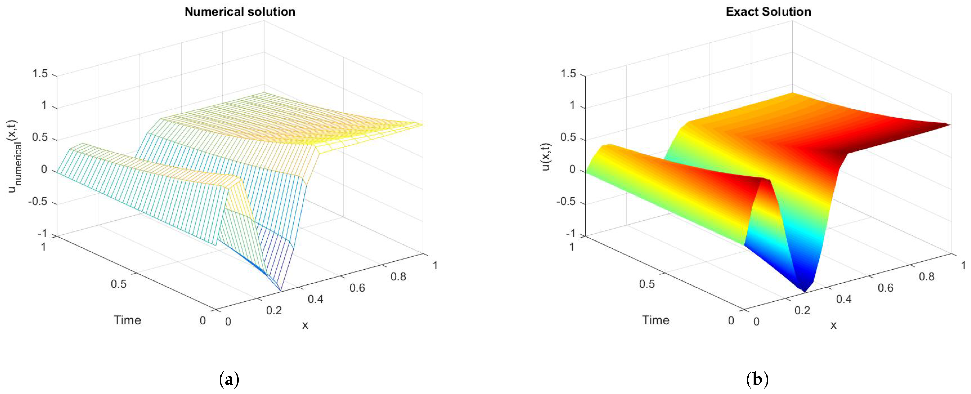
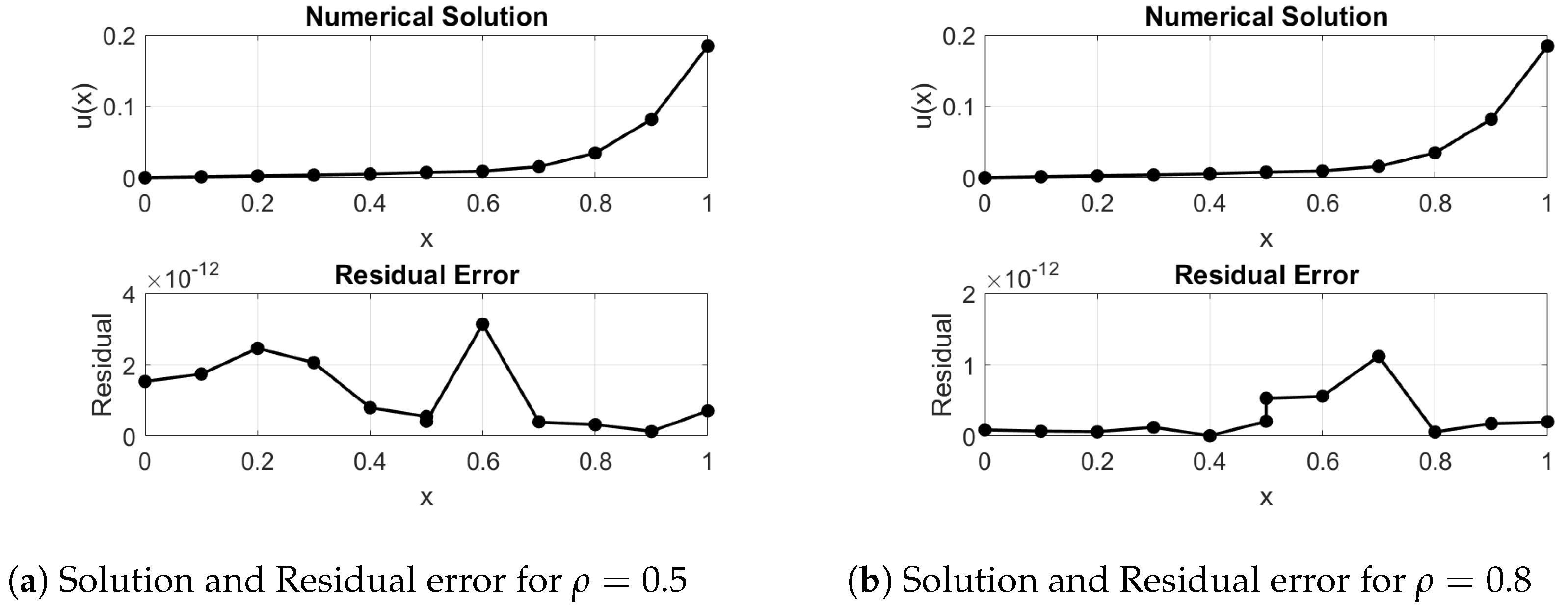
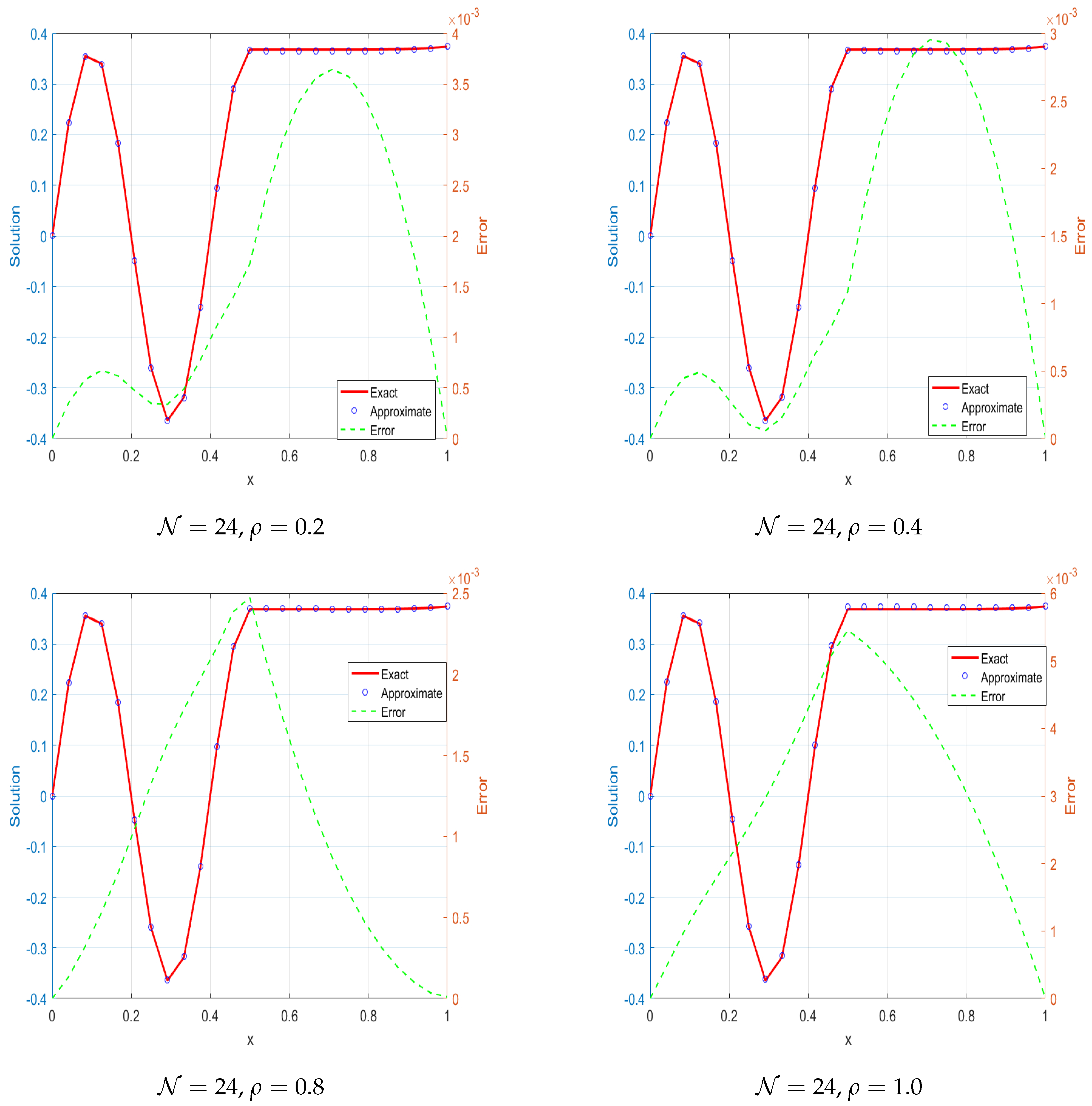
Example 4.

As the fourth example, we present the 1D time-fractional interface Problem 1 with its initial and boundary conditions, for which no exact solution is available:

$$\begin{array}{ccc}\hfill {\phi }_1(0,t)& =0, \hfill & \hfill (x,t)\in \partial \mathsf{\Omega }\times (0,T_f],\\ \hfill {\phi }_2(1,t)& ={\displaystyle \frac{257}{512}} e^{-t}, \hfill & \hfill (x,t)\in \partial \mathsf{\Omega }\times (0,T_f],\\ \hfill {\phi }_1(x,0)& =0, \hfill & \hfill x\in \mathsf{\Omega },\\ \hfill {\phi }_2(x,0)& =x^8, \hfill & \hfill x\in \mathsf{\Omega }.\end{array}$$

(42)

We use the residual error to assess the effectiveness of the suggested MQ-RBF scheme because there is no exact solution for this problem. The residual errors for various values of ρ are reported in

Table 4. Residual errors for various values of $\rho$ with $ϵ=1$, using MQ-RBFs at $d\mathsf{t}=0.5$ and $\mathsf{t}=1$ for Example 4.

$\mathsf{\rho }$	Metric	$\mathcal{N}$
		2	4	8	10
0.2	Residual error	2.6769 × 10−17	1.7494 × 10−15	5.8045 × 10−13	1.2052 × 10−11
0.5	Residual error	2.6769 × 10−17	1.1700 × 10−15	9.9245 × 10−13	5.2365 × 10−12
0.8	Residual error	2.6769 × 10−17	1.8374 × 10−15	2.3241 × 10−13	1.4119 × 10−12
1.0	Residual error	2.6769 × 10−17	2.5108 × 10−15	9.5667 × 10−13	7.5988 × 10−12

, demonstrating that the technique consistently produces modest residuals even for coarse discretizations. Plotting the numerical solution and associated residual error for $\rho =0.5$ and $\rho =0.8$ (see Figure 7) allows us to further evaluate the accuracy and validate the stability and dependability of the suggested method.

Example 5.

As the fifth example, nonlinear time-fractional interface Problem (1) is considered assuming ${\eta }^{+}\left(x\right)=1$ and ${\eta }^{-}\left(x\right)=2$. Exact solutions and source functions are given by

$$\phi (x,t)=\left\{\begin{array}{cc}{\phi }_1(x,t)=x^8{e}^{-t},\hfill & 0\le x\le {\displaystyle \frac{1}{2}},\hfill \\ {\phi }_2(x,t)={\displaystyle \frac{1}{2}}\left(x^8+{\displaystyle \frac{1}{256}}\right)e^{-t},\hfill & {\displaystyle \frac{1}{2}}\le x\le 1.\hfill \end{array}\right.$$

(43)

and

$$f(x,t)=\left\{\begin{array}{cc}{f}_1(x,t)=-2x^{16}{e}^{-2t}-56x^6{e}^{-t}-t^{1-\rho }{\mathcal{M}}_{1,2-\rho }(-t)x^8,\hfill & 0\le x\le {\displaystyle \frac{1}{2}},\hfill \\ f_2(x,t)=-{\displaystyle \frac{1}{2}}{t}^{1-\rho }{\mathcal{M}}_{1,2-\rho }(-t)(x^8+{\displaystyle \frac{1}{256}})-{\left(x^8+{\displaystyle \frac{1}{256}}\right)}^2{e}^{-2t}-56x^6{e}^{-t}{e}^{-t},\hfill & {\displaystyle \frac{1}{2}}\le x\le 1,\hfill \end{array}\right.$$

(44)

where ${\mathcal{M}}_{a,b}(·)$ is the Mittag–Leffler function of two parameters defined as

$${\mathcal{M}}_{a,b}\left(t\right)=\sum _{k=0}^{\infty }{\displaystyle \frac{t^k}{\mathsf{\Gamma }(ak+b)}}, \forall t\in \mathbb{C}, a,b\in {\mathbb{R}}^{+}$$

and

$${\mathcal{M}}_{1,1}\left(t\right)=exp\left(t\right), \forall t\in \mathbb{C}.$$

To formulate the computational problem, the exact analytical solution is used to define the initial, boundary, and interface conditions. The MQ-RBF method is then applied to the nonlinear 1D time-fractional interface model, using both quasi-Newton linearization and a new splitting technique to address the nonlinear terms.

Table 5. Error analysis for different values of $\rho$ and $\mathcal{N}$ with $ϵ=2$, $dt=0.5$, and $t=1$ for Example 5 using Caputo derivative and qausi-Newton linearization technique.

$\mathcal{N}$	$\mathsf{\rho }=0.7$		$\mathsf{\rho }=0.8$		$\mathsf{\rho }=0.9$		$\mathsf{\rho }=1$
	MAEs	RMSEs	MAEs	RMSEs	MAEs	RMSEs	MAEs	RMSEs
2	8.5612 × 10−2	6.0537 × 10−2	8.5612 × 10−2	6.0537 × 10−2	8.5612 × 10−2	6.0537 × 10−2	8.5612 × 10−2	6.0537 × 10−2
4	2.1732 × 10−2	1.0156 × 10−2	2.1817 × 10−2	1.0164 × 10−2	2.1911 × 10−2	1.0173 × 10−2	2.2013 × 10−2	1.0181 × 10−2
8	1.1155 × 10−2	6.5406 × 10−3	1.1135 × 10−2	6.5366 × 10−3	1.1086 × 10−2	6.5156 × 10−3	1.1005 × 10−2	6.4755 × 10−3
12	3.4876 × 10−3	1.9800 × 10−3	3.4103 × 10−3	1.9385 × 10−3	3.3101 × 10−3	1.8855 × 10−3>	3.1859 × 10−3	1.8215 × 10−3
16	7.8297 × 10−4	3.7803 × 10−4	8.9016 × 10−4	4.1823 × 10−4	1.0152 × 10−3	4.8017 × 10−4	1.1771 × 10−3	5.6466 × 10−4

and

Table 6. Error analysis for different values of $\rho$ and $\mathcal{N}$ with $\omega =1$, $ϵ=2$, $dt=0.5$, and $t=1$ for Example 5 using Caputo derivative and innovative splitting technique technique.

$\mathcal{N}$	$\mathsf{\rho }=0.7$		$\mathsf{\rho }=0.8$		$\mathsf{\rho }=0.9$		$\mathsf{\rho }=1$
	MAEs	RMSEs	MAEs	RMSEs	MAEs	RMSEs	MAEs	RMSEs
2	8.5612 × 10−2	6.0537 × 10−2	8.5612 × 10−2	6.0537 × 10−2	8.5612 × 10−2	6.0537 × 10−2	8.5612 × 10−2	6.0537 × 10−2
4	2.0914 × 10−2	1.0159 × 10−2	2.0992 × 10−2	1.0164 × 10−2	2.1079 × 10−2	1.0169 × 10−2	2.1174 × 10−2	1.0174 × 10−2
8	1.1478 × 10−2	6.7338 × 10−3	1.1463 × 10−2	6.7323 × 10−3	1.1419 × 10−2	6.7136 × 10−3	1.1345 × 10−2	6.6758 × 10−3
12	3.8849 × 10−3	2.2278 × 10−3	3.8149 × 10−3	2.1863 × 10−3	3.7225 × 10−3	2.1319 × 10−3	3.6061 × 10−3	2.0643 × 10−3
16	7.6333 × 10−4	4.3586 × 10−4	6.6953 × 10−4	4.0632 × 10−4	6.3176 × 10−4	3.8792 × 10−4	7.6948 × 10−4	3.9305 × 10−4

show that for various fractional orders ρ and discretization levels $\mathcal{N}$, the MAEs and RMSEs consistently decrease as $\mathcal{N}$ increases, confirming the accuracy and convergence of the scheme. Although the method performs well for all values of ρ, smaller fractional orders yield slightly higher errors due to stronger memory effects. A comparison of the two linearization strategies indicates that the proposed splitting technique is more accurate and converges faster than the quasi-Newton method. This improvement results from its better handling of nonlinearities while maintaining numerical stability. A more direct comparison can be made by selecting the cases with the largest error reduction. At $\mathcal{N}=16$ and $\rho =0.9$, the innovative splitting technique yields an MAE of $6.3176\times {10}^{-04}$, which is approximately 38% lower than the MAE $1.0152\times {10}^{-03}$ from the quasi-Newton method. Similarly, for $\mathcal{N}=16$ and $\rho =0.8$, the splitting method achieves an MAE of $6.6953\times {10}^{-04}$, showing an improvement of about 25% compared to the quasi-Newton MAE $8.9016\times {10}^{-04}$. We also computed the errors for different values of the parameter ω for the splitting method, and the results help in identifying the optimal choice of ω from

Table 7. Error analysis for various values of the relaxation parameter $\omega$ at fixed $N=20$ and $ϵ=1$ using the Caputo-based splitting technique, with $d\mathsf{t}=0.5$ and $\mathsf{t}=1$ for test Problem 5.

$\mathsf{\rho }$	Metric	$\mathsf{\omega }$
		−1	0	0.5	1	1.5
0.2	MAEs	8.3706 × 10−4	2.1501 × 10−4	8.4754 × 10−5	3.7093 × 10−4	6.5046 × 10−4
	RMSEs	5.7968 × 10−4	1.4800 × 10−4	5.8171 × 10−5	2.5718 × 10−4	4.5001 × 10−4
0.5	MAEs	9.9082 × 10−4	3.4900 × 10−4	6.3616 × 10−5	2.6409 × 10−4	5.4860 × 10−4
	RMSEs	6.8870 × 10−4	2.3895 × 10−4	2.9805 × 10−5	1.8437 × 10−4	3.8424 × 10−4
0.8	MAEs	1.3257 × 10−3	6.5940 × 10−4	3.5077 × 10−4	9.9970 × 10−5	2.9770 × 10−4
	RMSEs	9.2218 × 10−4	4.4944 × 10−4	2.2679 × 10−4	4.2454 × 10−5	2.0825 × 10−4
1	MAEs	1.6530 × 10−3	9.7078 × 10−4	6.4876 × 10−4	3.5666 × 10−4	1.3108 × 10−4
	RMSEs	1.1503 × 10−3	6.6266 × 10−4	4.3229 × 10−4	2.1356 × 10−4	6.5287 × 10−5

. Figure 8 provides a two-dimensional error comparison of the methods, and additional figures (e.g., Figure 9) show the impact of varying $\mathcal{N}$ for a fixed ρ.

Example 6.

As the sixth example, nonlinear time-fractional interface Problem (2) is considered assuming ${\eta }^{+}\left(x\right)=e^{(-10{(x-0.5)}^4{x}^4)}$ and ${\eta }^{-}\left(x\right)=3$. Exact solutions and source functions are given by

$$\phi (x,t)=\left\{\begin{array}{cc}{\phi }_1(x,t)=sin5\pi x{e}^{-t},\hfill & 0\le x\le {\displaystyle \frac{1}{2}},\hfill \\ {\phi }_2(x,t)=(2{(x-{\displaystyle \frac{1}{2}})}^7+1)e^{-t},\hfill & {\displaystyle \frac{1}{2}}\le x\le 1.\hfill \end{array}\right.$$

(45)

and

$$f(x,t)=\left\{\begin{array}{c}{f}_1(x,t)=-t^{1-\rho }{\mathcal{M}}_{1,2-\rho }(-t)sin\left(5\pi x\right)+15\pi e^{-t-10x^4{(x-{\displaystyle \frac{1}{2}})}^4}cos\left(5\pi x\right)(40x^3{(x-{\displaystyle \frac{1}{2}})}^4\hfill \\ +40x^4{(t-{\displaystyle \frac{1}{2}})}^3)-{\left(sin5\pi x e^{-t}\right)}^2-2{sin}^{2}5\pi x e^{-2t},\hfill & 0\le x\le {\displaystyle \frac{1}{2}},\hfill \\ f_2(x,t)=-t^{1-\rho }{\mathcal{M}}_{1,2-\rho }(-t)\left(2{(x-{\displaystyle \frac{1}{2}})}^7+1\right)-252e^{(-t){(x-{\displaystyle \frac{1}{2}})}^5}\hfill \\ -2{\left(2{\left(x-{\displaystyle \frac{1}{2}}\right)}^7+1\right)}^2{e}^{-2t},\hfill & {\displaystyle \frac{1}{2}}\le x\le 1,\hfill \end{array}\right.$$

(46)

where ${\mathcal{M}}_{a,b}(·)$ is the Mittag–Leffler function of two parameters defined as

$${\mathcal{M}}_{a,b}\left(t\right)=\sum _{k=0}^{\infty }{\displaystyle \frac{t^k}{\mathsf{\Gamma }(ak+b)}}, \forall t\in \mathbb{C}, a,b\in {\mathbb{R}}^{+}$$

and

$${\mathcal{M}}_{1,1}\left(t\right)=exp\left(t\right), \forall t\in \mathbb{C}.$$

To accurately define the interface, boundary, and initial conditions for this nonlinear 1D time-fractional interface problem, the exact analytical solution is employed as a reference. The MQ-RBFs, enhanced by a novel splitting approach to efficiently manage the nonlinearity, is utilized to obtain the numerical solution. Computational experiments, detailed in

Table 8. Error analysis for different values of $\rho$ and $\mathcal{N}$ with $\omega =1$, $ϵ=2$, $dt=0.5$ and $t=1$ for Example 6 using Caputo derivative and innovative splitting technique.

$\mathcal{N}$	$\mathsf{\rho }=0.2$		$\mathsf{\rho }=0.5$		$\mathsf{\rho }=0.8$
	MAEs	RMSEs	MAEs	RMSEs	MAEs	RMSEs
8	6.9074 × 10−1	4.2324 × 10−1	6.9322 × 10−1	4.2492 × 10−1	6.9317 × 10−1	4.2484 × 10−1
12	1.1365 × 10−1	7.2496 × 10−2	1.1635 × 10−1	7.4379 × 10−2	1.2075 × 10−1	7.7448 × 10−2
16	4.4815 × 10−2	2.7262 × 10−2	4.6980 × 10−2	2.8794 × 10−2	5.0937 × 10−2	3.1612 × 10−2
20	1.2059 × 10−2	7.4183 × 10−3	1.4047 × 10−2	8.7274 × 10−3	1.8119 × 10−2	1.1376 × 10−2
24	5.5964 × 10−3	3.5535 × 10−3	7.0617 × 10−3	4.3015 × 10−3	1.0958 × 10−2	6.4125 × 10−3

, explore the performance of the method across various fractional orders $\rho$ and spatial resolutions $\mathcal{N}$. The accuracy of the approach is quantitatively assessed using mean MAEs and RMSEs, both of which consistently decline as the grid becomes finer, indicating strong convergence behavior. While the method remains stable and reliable for all considered values of $\rho$, lower fractional orders tend to yield higher errors, reflecting the intensified memory effects inherent to the fractional derivative. Overall, the results affirm the precision and robustness of the MQ-RBFs in addressing nonlinear time-fractional interface problems. In Figure 10 we have plotted 2D plots for different values of $\rho$, along with the corresponding errors.

7. Conclusions

This study presents a new numerical method called MQ-RBF, developed to solve both linear and nonlinear time-fractional interface problems involving constant and variable coefficients. The method uses the Caputo definition of fractional derivatives, where the first-order time derivatives are approximated using a finite difference scheme. To effectively manage nonlinearity, an innovative splitting technique and the quasi-Newton linearization method are implemented. The innovative splitting technique produced more accurate and stable results than quasi-Newton linearization, particularly in capturing the dynamic behavior of the solution. This enhancement is due to the splitting technique’s superior capability in handling nonlinear interactions while preserving numerical accuracy. A key advantage of the MQ-RBF method is that it achieves high accuracy using only a small number of grid points, making it computationally efficient. The effectiveness of the MQ-RBF method is demonstrated through several benchmark test cases, which include both constant and variable coefficient problems. The results show that the method delivers highly accurate solutions, as measured by the MAEs and RMSEs with different fractional-order values ($\rho$). Visualizations in 2D and 3D further illustrate how the solution evolves over time and with varying $\rho$. In general, the proposed MQ-RBF method is shown to be accurate and efficient. Future work may explore extending it to two and three-dimensional time-fractional interface problems, including cases with single or multiple interfaces.