Application of Generalized Finite Difference Method and Radial Basis Function Neural Networks in Solving Inverse Problems of Surface Anomalous Diffusion

Abstract

In this study, a new hybrid method based on the generalized finite difference method (GFDM) and radial basis function (RBF) neural network technologies is developed to solve the inverse problems of surface anomalous diffusion. Specifically, the GFDM is utilized to compute the time-fractional derivative model on the surface, whereas RBF neural networks are employed to invert the diffusion coefficient, source term coefficient, and the fractional order within the anomalous diffusion equation governing the surface. The results of four examples show that for the three parameters of diffusion coefficient, source term coefficient, and fractional order, the errors of inversion results are in the order of $10^{-2}$ under different conditions. Therefore, this method can obtain the required parameters quickly and accurately under different conditions.

1. Introduction

Since the 1980s, advancements in science and technology have led to the gradual revelation of a series of physical phenomena known as anomalous diffusion [1,2,3,4]. These phenomena are complex and difficult to fully explain or accurately model using traditional integer-order diffusion systems. Anomalous diffusion has been demonstrated in various fields, including porous media mechanics [5], non-Newtonian fluid mechanics [6], viscoelastic mechanics [7], and soft matter mechanics [8,9]. The fractional diffusion model [10] is one of the most common models to describe anomalous diffusion behavior. Its advantage lies in its simpler parameters and more convenient numerical calculations. The non-local properties of fractional derivatives [11] enable them to describe complex non-Markov systems [12].

Due to the non-local characteristics and complexity of fractional differential equations [11], obtaining analytical solutions for these equations is extremely challenging. Therefore, developing efficient and accurate numerical algorithms to solve fractional differential equations is crucial. In recent years, numerous meshless methods have been proposed. These methods replace the traditional grid with nodes, thereby avoiding the complicated grid generation process. 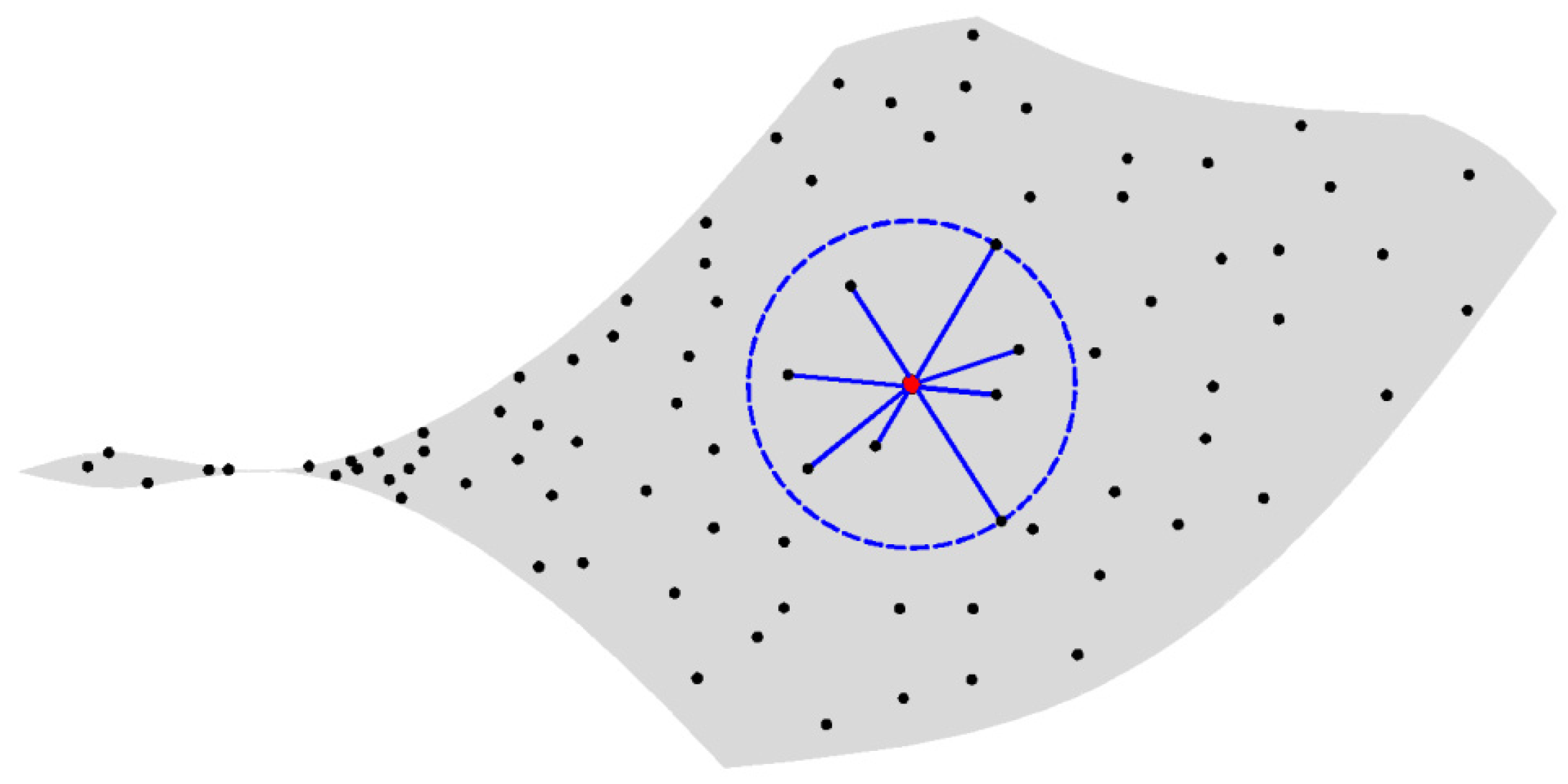Meshless methods include the fundamental solution method [13], Trefftz method [14], singular boundary method [15], generalized finite difference method [16,17], etc. The GFDM is a relatively new localized meshless method. First proposed by T. Liszka and J. Orkisz in the 1980s [18], it has been continuously improved and refined until a relatively complete version was proposed by Benito et al. in 2001 [19]. The GFDM has been successfully applied in many fields due to its ability to overcome the constraints of traditional regular grids and its capacity to handle complex boundary conditions without the need for extensive preprocessing. Moreover, its localized configuration makes it particularly suitable for dealing with large-scale problems, including obstacle problems [20], inverse problems [21], slogging phenomena [22], etc.

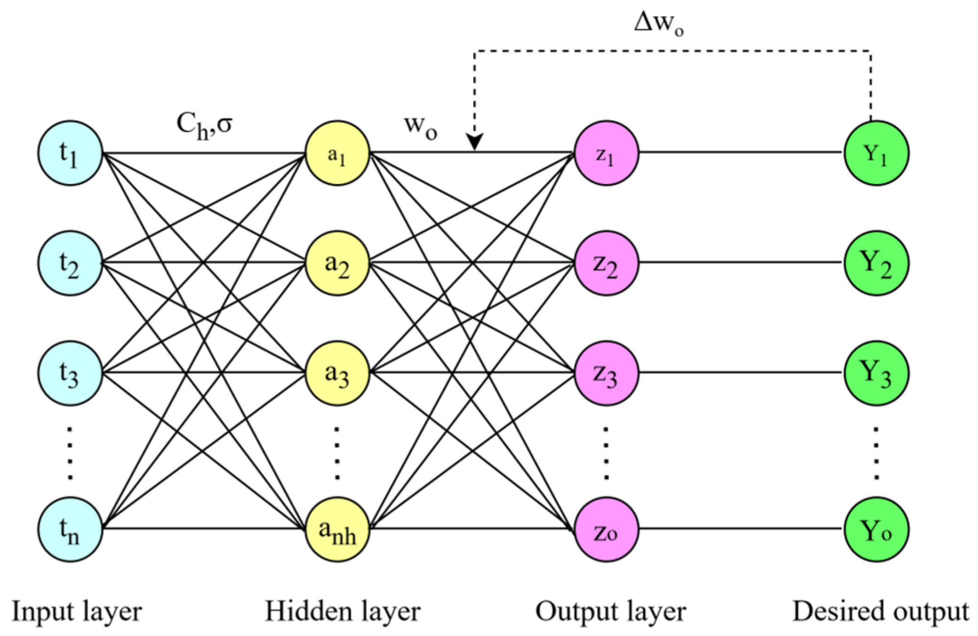
In recent years, with the rapid development of neural network technology, using neural networks to solve inverse problems of anomalous diffusion equations has become increasingly prevalent [23,24,25,26]. The RBF neural network is a relatively advanced type of three-layer feedforward neural network. Compared with back-propagation (BP) neural networks, RBF neural networks exhibit superior performance in classification accuracy, learning speed, and approximation ability [27]. An RBF neural network is a kind of neural network with local approximation performance, so an RBF neural network is faster in inversion than other neural networks. In addition, an RBF neural network can accurately invert the results when dealing with the problems in this paper, so an RBF neural network is adopted to invert the parameters.

Compared with other work, this is the first time the inverse surface diffusion problem is solved by combining GFDM and RBF neural networks. In this paper, the time-fractional derivative model is introduced to define the anomalous diffusion process on the surface. In the numerical implementation, the GFDM and the extrinsic processing technique of the surface partial differential equation are employed for the discrete solution. Subsequently, RBF neural networks are introduced into the inverse problem of inverting diffusion equation parameters to obtain the required equation parameters. Specifically, a training database is established by solving the proposed time-fractional diffusion equation using the GFDM.

2. The GFDM in Solving Anomalous Diffusion on the Surface

2.1. Time-Fractional Derivative Model on the Surface

To address the intricate issue of anomalous diffusion on a surface, the time-fractional derivative model is introduced. Given that S represents a closed and smooth surface within a three-dimensional space, the fractional diffusion equation formulated on this surface can be articulated as follows:

$${\displaystyle \frac{{𝜕}^{\alpha }u\left(\mathbf{x},t\right)}{𝜕t^{\alpha }}}=\left(D{\Delta }_s+\overrightarrow{\nu }\cdot {\nabla }_s-\lambda \right)u\left(\mathbf{x},t\right)+Q\left(\mathbf{x},t\right),0<\alpha <1,\mathbf{x}\in S,t\in \left(0,T\right),$$

(1)

and the following initial condition is given as

$$u\left(\mathbf{x},0\right)=u_0\left(\mathbf{x}\right),\mathbf{x}\in S,$$

(2)

where $D$, $\lambda$, and $\overrightarrow{\nu }$ represent diffusion coefficient, reaction coefficient, and velocity vector, respectively. $Q(\mathbf{x},t)$ and $u_0\left(\mathbf{x}\right)$ are known functions, $T$ is the total time, ${\Delta }_s$ and ${\nabla }_s$ represent the Laplace–Beltrami and surface gradient operators, respectively [28]. ${𝜕}^{\alpha }/𝜕t^{\alpha }$ is the Caputo time-fractional of order $\alpha$ with respect to $t$ [29], which is defined by the following equation:

$${\displaystyle \frac{{𝜕}^{\alpha }u\left(\mathbf{x},t\right)}{𝜕t^{\alpha }}}={\displaystyle \frac{1}{\mathsf{\Gamma }\left(1-\alpha \right)}}{\int }_0^t{\displaystyle \frac{𝜕u\left(\mathbf{x},\eta \right)}{𝜕\eta }}{\displaystyle \frac{d\eta }{{\left(t-\eta \right)}^{\alpha }}},0<\alpha <1,$$

(3)

where $\mathsf{\Gamma }$ is the Gamma function. By using the standard finite difference method, the time-fractional derivative model can be discretized as [30]

$$\begin{array}{c}D\theta {\Delta }_s{u}^{k+1}+\theta \overrightarrow{\nu }\cdot {\nabla }_s{u}^{k+1}-\left(\lambda \theta +{\alpha }_0\right)u^{k+1}=\\ \left\{\begin{array}{c}\begin{array}{c}-\theta Q^{k+1}-\left(1-\theta \right)\left(D{\Delta }_s{u}^k+\overrightarrow{\nu }\cdot {\nabla }_s{u}^k+Q^k-\lambda u^k\right)\\ -{\alpha }_0{u}^k+{\sum }_{j=1}^k{\alpha }_j{b}_j\left(u^{k-j+1}-u^{k-j}\right),k\ge 1, \end{array}\\ -\theta Q^1-\left(1-\theta \right)\left(D{\Delta }_s{u}^0+\overrightarrow{\nu }\cdot {\nabla }_s{u}^0+Q^0-\lambda u^0\right)-{\alpha }_0{u}^0,k=0.\end{array}\right.\end{array}$$

(4)

where ${\alpha }_j$ and $b_j$ are known coefficients, and $\theta$ is the time integral constant. $a_0={\displaystyle \frac{{dt}^{-\alpha }}{\mathsf{\Gamma }\left(1+\alpha \right)}}$, where $dt$ is the time step.

2.2. Surface Differential Operators

Suppose $S$ is a closed and smooth surface defined in three-dimensional space, and for an arbitrary point ${\mathbf{x}}_i={\left[x_i,y_i,z_i\right]}^T$ on this surface, the normal vector at this point is expressed as $\mathbf{n}=\mathbf{n}\left(\mathbf{x}\right)={\left[n_{x_i},n_{y_i},n_{z_i}\right]}^T$. Then, the surface gradient operator at x can be formulated as follows:

$${\nabla }_s=\mathbf{P}\nabla =\left({\mathbf{I}}_3-\mathbf{n}{\mathbf{n}}^T\right)\nabla ,$$

(5)

where ${\mathbf{I}}_d$ is a $d\times d$ identity matrix and $\mathbf{P}$ represents the projection matrix. The Laplace–Beltrami operator at $\mathbf{x}$ can be expressed as

$${\Delta }_s={\nabla }_s\cdot {\nabla }_s.$$

(6)

By introducing the extrinsic technique, the analytical relationship between the operators defined in tangent space and the operators defined in Euclidean space can be derived from the normal vector $\mathbf{n}$ corresponding to all points ${\mathbf{x}}_i$ selected on the surface [26]:

$${\nabla }_{s}u=\nabla u-\mathbf{n}{𝜕}_{\mathbf{n}}u,{\Delta }_{s}u=\Delta u-H_s{𝜕}_{\mathbf{n}}u-{𝜕}_{\mathbf{n}}^{\left(2\right)}u.$$

(7)

where ${𝜕}_{\mathbf{n}}u={\mathbf{n}}^T\nabla u$, ${𝜕}_{\mathbf{n}}^{\left(2\right)}u={\mathbf{n}}^{T}J\left(\nabla u\right)\mathbf{n}$, and $H_s\left(x\right)=trace\left(J\left(\mathbf{n}\right)\left({\mathbf{I}}_d-\mathbf{n}{\mathbf{n}}^T\right)\right)$, and $J$ represents the jacobian operators in Euclidean space.

2.3. GFDM for Time-Fractional Derivative Model on the Surface

Similar to traditional finite difference methods, the generalized finite difference method constructs numerical differential formulas to approximate partial derivative terms of partial differential equations. The general formula can be expressed as follows:

$$D_u=WU,$$

(8)

where the partial derivative vector $D_u$, the weighting matrix $W$, and the solution vector $U$ are, respectively, defined as

$$D_u={{\left[\begin{array}{ccc}{\displaystyle \frac{𝜕u_i}{𝜕x_k}},& \dots \dots & ,{\displaystyle \frac{{𝜕}^2{u}_i}{𝜕x_k𝜕x_{k^{″}}}}\end{array}\right]}_{1\times n_v}}^T,k=\mathrm{1,2},\dots \dots ,d;k^{″}=k,k+1,\dots \dots ,d,$$

(9)

$$U={\left[u_1,u_2,\dots \dots ,u_N\right]}^T,$$

(10)

$$W={\left[\begin{array}{ccc}{\omega }_1^{x_k,i}& \cdots & {\omega }_N^{x_k,i}\\ ⋮& \ddots & ⋮\\ {\omega }_1^{x_k{x}_{k^{″}},i}& \cdots & {\omega }_N^{x_k{x}_{k^{″}},i}\end{array}\right]}_{n_v\times N},k=\mathrm{1,2},\dots ,d;k^{″}=k,k+1,\dots ,d.$$

(11)

where $d$ represents the dimension, $u_i\left(i=\mathrm{1,2},\dots ,N\right)$ is the solution of the discretized node $x_i$, $x_i=\left(x_{i1},x_{i2},\dots ,x_{id}\right)\in \Xi \subset R^d$, and $n_v=2d+C_d^2$.

The GFDM, which is defined in Euclidean space, can be directly employed for approximating surface differential operators with extrinsic technology. Figure 1 shows a sketch of discrete points of the computational domain and neighborhood selection using the meshless generalized finite difference method, and the equation for the GFDM is provided as follows:

$$\left\{\begin{array}{c}\begin{array}{c}{\displaystyle \frac{𝜕u_{x^{\xi }}}{𝜕x}}=W_{x_i}{u}_i+{\sum }_{j=1}^N{W}_{x_j}{u}_j,\\ {\displaystyle \frac{𝜕u_{y^{\xi }}}{𝜕y}}=W_{y_i}{u}_i+{\sum }_{j=1}^N{W}_{y_j}{u}_j,\\ {\displaystyle \frac{𝜕u_{z^{\xi }}}{𝜕z}}=W_{z_i}{u}_i+{\sum }_{j=1}^N{W}_{z_j}{u}_j,\end{array}\\ \begin{array}{c}{\displaystyle \frac{𝜕u_{x^{\xi }}}{𝜕x^2}}=W_{x_i{x}_i}{u}_i+{\sum }_{j=1}^N{W}_{x_j{x}_j}{u}_j,\\ {\displaystyle \frac{𝜕u_{y^{\xi }}}{𝜕y^2}}=W_{y_i{y}_i}{u}_i+{\sum }_{j=1}^N{W}_{y_j{y}_j}{u}_j,\\ {\displaystyle \frac{𝜕u_{z^{\xi }}}{𝜕z^2}}=W_{z_i{z}_i}{u}_i+{\sum }_{j=1}^N{W}_{z_j{z}_j}{u}_j,\end{array}\\ \begin{array}{c}{\displaystyle \frac{𝜕u_{x^{\xi }{y}^{\xi }}}{𝜕x𝜕y}}=W_{x_i{y}_i}{u}_i+{\sum }_{j=1}^N{W}_{x_j{y}_j}{u}_j,\\ {\displaystyle \frac{𝜕u_{x^{\xi }{z}^{\xi }}}{𝜕x𝜕z}}=W_{x_i{z}_i}{u}_i+{\sum }_{j=1}^N{W}_{x_j{z}_j}{u}_j,\\ {\displaystyle \frac{𝜕u_{y^{\xi }{z}^{\xi }}}{𝜕y𝜕z}}=W_{y_i{z}_i}{u}_i+{\sum }_{j=1}^N{W}_{y_j{z}_j}{u}_j.\end{array}\end{array}\right.$$

(12)

where $x, y, z$ are the Euclidian coordinates. Thus, the unified equation can be derived as

$$Lu{|}_{x^{\xi }}=W^{\xi }{U}^{\xi },$$

(13)

where $L$ represents any differential operator, $W^{\xi }$ represents the row vector of $1\times N_s$, and $U^{\xi }$ represents the column vector of the local solution of $N_s\times 1$. If $S$ is a smooth closed surface, then ${\nabla }_{s}u$ can be expressed as

$${\nabla }_{s}u=\mathbf{P}\cdot \nabla u=\mathbf{P}\left[\begin{array}{c}{\displaystyle \frac{𝜕u}{𝜕x}}\\ {\displaystyle \frac{𝜕u}{𝜕y}}\\ {\displaystyle \frac{𝜕u}{𝜕z}}\end{array}\right]=\left[\begin{array}{c}{p}_{11}{\displaystyle \frac{𝜕u}{𝜕x}}+p_{12}{\displaystyle \frac{𝜕u}{𝜕y}}+p_{13}{\displaystyle \frac{𝜕u}{𝜕z}}\\ p_{21}{\displaystyle \frac{𝜕u}{𝜕x}}+p_{22}{\displaystyle \frac{𝜕u}{𝜕y}}+p_{23}{\displaystyle \frac{𝜕u}{𝜕z}}\\ p_{31}{\displaystyle \frac{𝜕u}{𝜕x}}+p_{32}{\displaystyle \frac{𝜕u}{𝜕y}}+p_{33}{\displaystyle \frac{𝜕u}{𝜕z}}\end{array}\right].$$

(14)

${\Delta }_{s}u$ can be expressed as

$$\begin{array}{c}\begin{array}{c}{\Delta }_{s}u{|}_{x^{\xi }}=\left(W_{x_1{x}_1}^{\xi }+W_{x_2{x}_2}^{\xi }+W_{x_3{x}_3}^{\xi }\right)U^{\xi }-H_S\left(x^{\xi }\right)\left[n_{x_1}^{\xi }{n}_{x_2}^{\xi }{n}_{x_3}^{\xi }\right]\left[\begin{array}{c}{W}_{x_1}^{\xi }\\ W_{x_2}^{\xi }\\ W_{x_3}^{\xi }\end{array}\right]U^{\xi }\\ \end{array}\\ -\left[n_{x_1}^{\xi }{n}_{x_2}^{\xi }{n}_{x_3}^{\xi }\right]\left[\begin{array}{ccc}{W}_{x_1{x}_1}^{\xi }& W_{x_1{x}_2}^{\xi }& W_{x_1{x}_3}^{\xi }\\ W_{x_2{x}_1}^{\xi }& W_{x_2{x}_2}^{\xi }& W_{x_2{x}_3}^{\xi }\\ W_{x_3{x}_1}^{\xi }& W_{x_3{x}_2}^{\xi }& W_{x_3{x}_3}^{\xi }\end{array}\right]\left[\begin{array}{c}{n}_{x_1}^{\xi }\times {{\rm I}}_N\\ n_{x_2}^{\xi }\times {{\rm I}}_N\\ n_{x_3}^{\xi }\times {{\rm I}}_N\end{array}\right]U^{\xi }.\end{array}$$

(15)

By using the GFDM and substituting Equations (14) and (15) into Equation (4), the time-fractional derivative model can be discretized as

$$\begin{array}{c}D\theta W_{\Delta s}{u}^{k+1}+\theta \overrightarrow{\nu }\cdot \left[\begin{array}{c}{W}_{\nabla s}^x{u}^{k+1}\\ W_{\nabla s}^y{u}^{k+1}\\ W_{\nabla s}^z{u}^{k+1}\end{array}\right]-\left(\lambda \theta +{\alpha }_0\right)u^{k+1}=\\ \left\{\begin{array}{c}\begin{array}{c}-\theta Q^{k+1}-\left(1-\theta \right)\left(D{W}_{\Delta s}{u}^k+\overrightarrow{\nu }\cdot \left[\begin{array}{c}{W}_{\nabla s}^x{u}^k\\ W_{\nabla s}^y{u}^k\\ W_{\nabla s}^z{u}^k\end{array}\right]+Q^k-\lambda u^k\right)\\ -{\alpha }_0{u}^k+{\sum }_{j=1}^k{\alpha }_j{b}_j\left(u^{k-j+1}-u^{k-j}\right),k\ge 1,\end{array}\\ -\theta Q^1-\left(1-\theta \right)\left(D{W}_{\Delta s}{u}^0+\overrightarrow{\nu }\cdot \left[\begin{array}{c}{W}_{\nabla s}^x{u}^0\\ W_{\nabla s}^y{u}^0\\ W_{\nabla s}^z{u}^0\end{array}\right]+Q^0-\lambda u^0\right)-{\alpha }_0{u}^0,k=0.\end{array}\right.\end{array}$$

(16)

3. RBF Neural Networks

As shown in Figure 2, RBF neural networks, consisting of an input layer, one hidden layer, and an output layer, are one of the current famous artificial neural networks.

The training process comprises two pivotal steps: initially, employing the K-means clustering algorithm to determine the centers of the basis functions from the training dataset; subsequently, optimizing the weights connecting the hidden layer to the output layer by minimizing the objective function. This training methodology enables the RBF neural networks to adapt more rapidly and accurately to diverse datasets and task requirements.

The Gaussian radial basis function is selected as the activation function, and the equation is given as follows:

$$\phi \left(r\right)=e^{-{\displaystyle \frac{r^2}{2{\sigma }^2}}},$$

(17)

The output of the $h$-th hidden neuron is given as

$$a_h=\mathit{exp}\left(-{\displaystyle \frac{1}{2{\sigma }^2}}{‖{\mathbf{C}}_h-\mathbf{t}‖}^2\right),$$

(18)

where $\mathbf{t}={\left(t_1,t_2,\cdots ,t_n\right)}^T$ is the input vector of the coefficients of the diffusion system equation from each detection point. The detection point will be selected from the GFDM nodes, and the input vector will be the spread value at that point in time. ${\mathbf{C}}_h$ and $\sigma$ are the neuron’s center and the center spread parameter, respectively.

For the $o$-th neuron, the output $z_o$ is

$$z_o={\sum }_{h=1}^{nh}{w}_o{a}_h+{\theta }_o,$$

(19)

where $nh$ is the number of neurons in the hidden layer. $w_o$ and ${\theta }_o$ are the weight and threshold connecting the neurons in the hidden layer to the neurons in the output layer.

The objective function is given as

$$J={\sum }_{o=1}^{no}{‖z_o-Y_o‖}^2,$$

(20)

The weights are modified by moving in the opposite direction to the gradient of the target function.

The adjustment formula is given as

$$\Delta w_o=-\mu {\displaystyle \frac{𝜕J}{𝜕w}}=\mu \left(z_o-Y_o\right)\mathit{exp}\left(-{\displaystyle \frac{1}{2{\sigma }^2}}{‖{\mathbf{C}}_h-\mathbf{t}‖}^2\right).$$

(21)

where $\Delta w_o$ represents the weight increments, and the constant $\mu$ represents the learning rate.

4. Numerical Results and Discussion

In this section, we combine the GFDM with the RBF neural networks to establish a parameter inversion model for the diffusion equation, based on the results of surface anomalous diffusion. Given that the RBF neural networks demonstrate higher accuracy than other artificial neural networks in parameter inversion, we verify the effectiveness and precision of the RBF neural networks in inverting diffusion coefficients based on surface anomalous diffusion results through the following examples.

In the numerical implementation, the neural network program is executed by MATLAB software R2016b through the ‘newrb’ function in the neural networks’ toolbox. The RBF neural networks iteratively create an RBF network using the function ‘newrb’, the target mean square error is set to 0.01, the radial basis function distribution coefficient is set to 1, the maximum number of neurons is set to 5000, and the number of neurons to be added between each display is set to 25. The optimization method is based on gradient descent.

In the parameter identification stage of the diffusion equation, the simulated diffusion results with an unknown diffusion coefficient at the observation point are input into the trained regression neural networks, and the corresponding parameters can be obtained. Different parameters are randomly generated in the detection domain, and the parameters are brought into the fractional diffusion equation on the surface after the GFDM. A large number of corresponding diffusion results and parameters are calculated as training samples for neural networks to learn. By constantly training and optimizing the weight parameters of the neural networks, a complex nonlinear mapping relationship between the features and labels of the training samples is constructed, and the trained neural networks can be used as a detection tool for the corresponding diffusion results and parameters.

The inversion error of diffusion equation parameters is given as

$$E={\displaystyle \frac{\left|X_{true}-X_{pred}\right|}{X_{true}}}\mathrm{\%}.$$

(22)

where $E$ is the error value, $X$ is the target parameter, $X_{true}$ is the true value of the target parameter, and $X_{pred}$ is the inversion value of the target parameter.

• Example 1.

Firstly, the inversion of the diffusion coefficient in the diffusion equation in the presence of analytical solutions is considered, and the GFDM approximation is used to invert the diffusion coefficient D. The fractional diffusion equation on a closed smooth surface in three-dimensional space is defined as Equation (1), where $D$ is the diffusion coefficient, $\alpha ={\displaystyle \frac{1}{2}}$, $Q\left(\mathit{x},t\right)=0$, and the analytical solution is given as

$$u\left(t,\mathbf{x}\right)=\mathit{sin}x\cdot \mathit{cos}y\cdot \mathit{tanh}z\cdot t,$$

(23)

In order to verify the accuracy, convergence, and stability of the GFDM for precisely capturing the anomalous diffusion phenomenon on the surface, Root Mean Square Error (RMSE) is introduced to measure it, and its equation is given as follows

$$RMSE\left(u_i\left(\mathbf{x},t\right)\right)=\sqrt{{\displaystyle \frac{1}{N}}{\sum }_{j=1}^N{\left[u\left({\mathbf{x}}_j,t\right)-\tilde{u}\left({\mathbf{x}}_j,t\right)\right]}^2}.$$

(24)

where $N$ represents the total number of discrete points of the surface, $\tilde{u}({\mathit{x}}_j,t)$ represents the numerical solution, and $u({\mathit{x}}_j,t)$ represents the analytical solution.

At the same time, RBF neural networks and BP neural networks are introduced to invert the parameters, so as to compare the advantages and disadvantages of the two methods in dealing with such problems. The hyperparameter settings are the same for both methods. There is no diffusion at the initial moment. From the initial moment, all the cloth points on the surface of the entire surface begin to diffuse at the same time. The time step is 0.01 s. Different diffusion coefficients are randomly generated in the detection domain, a point is randomly selected among the distribution points of the surface, and 30 points are randomly selected on the surface as observation points. 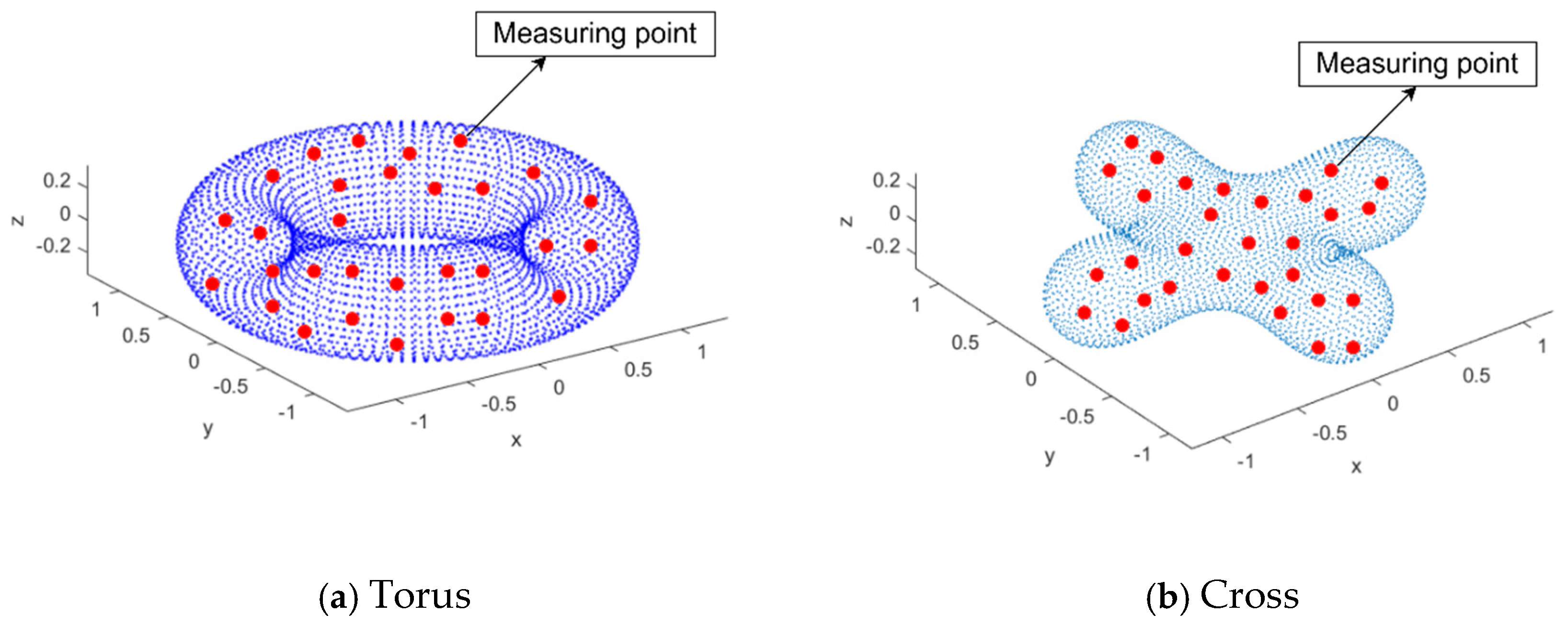The simulated diffusion results corresponding to diffusion coefficient D at the observation point of 0.1 s are taken as the input feature X of the neural networks and diffusion coefficient D is taken as the output Y, so that a sample $\left(X,Y\right)$ can be constructed. For two different shapes, torus and cross, the number of samples for each shape training is 1000 sets of data. Each set of data contains the diffusion values of thirty detection points at different times. Then, 70% of the samples are divided into a study set and 30% of the samples are divided into verification sets to evaluate the generalization ability of the neural networks. The number of samples for testing is four sets of data, and the test set is not involved in the training of the neural networks. Figure 3 shows the distribution of distribution points and measuring points when the surface is torus and ellipsoid.

Table 1. RMSE between numerical solution and analytical solution on different surfaces.

Shape	Sphere	Torus	Cross	RBC
N	2500	4000	3996	4096
RMSE	$2.73\times {10}^{-3}$	$1.16\times {10}^{-3}$	$2.50\times {10}^{-2}$	$3.46\times {10}^{-3}$

shows the RMSE between the GFDM approximation and the analytic solution on different surfaces at $t=0.1$.

Table 2. Inversion results, errors, and CPU time of RBFNN and BPNN with torus surface.

${\mathit{D}}_{\mathit{t}\mathit{r}\mathit{u}\mathit{e}}$	${\mathit{D}}_{\mathit{p}\mathit{r}\mathit{e}\mathit{d}}$		$\mathit{E}$ (%)		CPU Time (s)
	RBFNN	BPNN	RBFNN	BPNN	RBFNN	BPNN
0.2550	0.2552	0.2553	0.08	0.12	0.1	300
0.5050	0.5053	0.5054	0.06	0.08	0.1	305
0.7550	0.7526	0.7556	0.31	0.08	0.1	310
1.0050	1.0060	1.0061	0.10	0.11	0.1	306

and

Table 3. Inversion results, errors, and CPU time of RBFNN and BPNN with cross surface.

${\mathit{D}}_{\mathit{t}\mathit{r}\mathit{u}\mathit{e}}$	${\mathit{D}}_{\mathit{p}\mathit{r}\mathit{e}\mathit{d}}$		$\mathit{E}$ (%)		CPU Time (s)
	RBFNN	BPNN	RBFNN	BPNN	RBFNN	BPNN
0.2550	0.2538	0.2512	0.47	1.49	0.1	420
0.5050	0.5084	0.0535	0.67	0.51	0.1	415
0.7550	0.7536	0.7513	0.19	0.92	0.1	455
1.0050	1.0044	1.0094	0.06	0.35	0.1	435

, respectively, show the inversion results and errors of diffusion coefficients when the surface is torus and cross.

From Table 1, it can be observed that for different models, the RMSE is in the order of $10^{-2}$. The numerical results clearly demonstrate that the GFDM can precisely capture the anomalous diffusion phenomenon on the surface and accurately approximate analytical solutions. However, the limitation of GFDM is that it is difficult to obtain accurate results when it is used to deal with non-smooth, non-closed, and asymmetrical surface models. For future research, more widely used numerical methods may be needed to solve such problems, such as finite element methods.

From Table 2 and Table 3, it can be observed that for both methods, the predicted value of diffusion coefficient D is almost consistent with the actual value on different models. The error is in the order of $10^{-3}$. However, the inversion speed of an RBF neural network is significantly faster than that of a BP neural network. Therefore, the proposed model can achieve the fast and accurate inversion of diffusion coefficient D in the case of analytic solutions.

• Example 2.

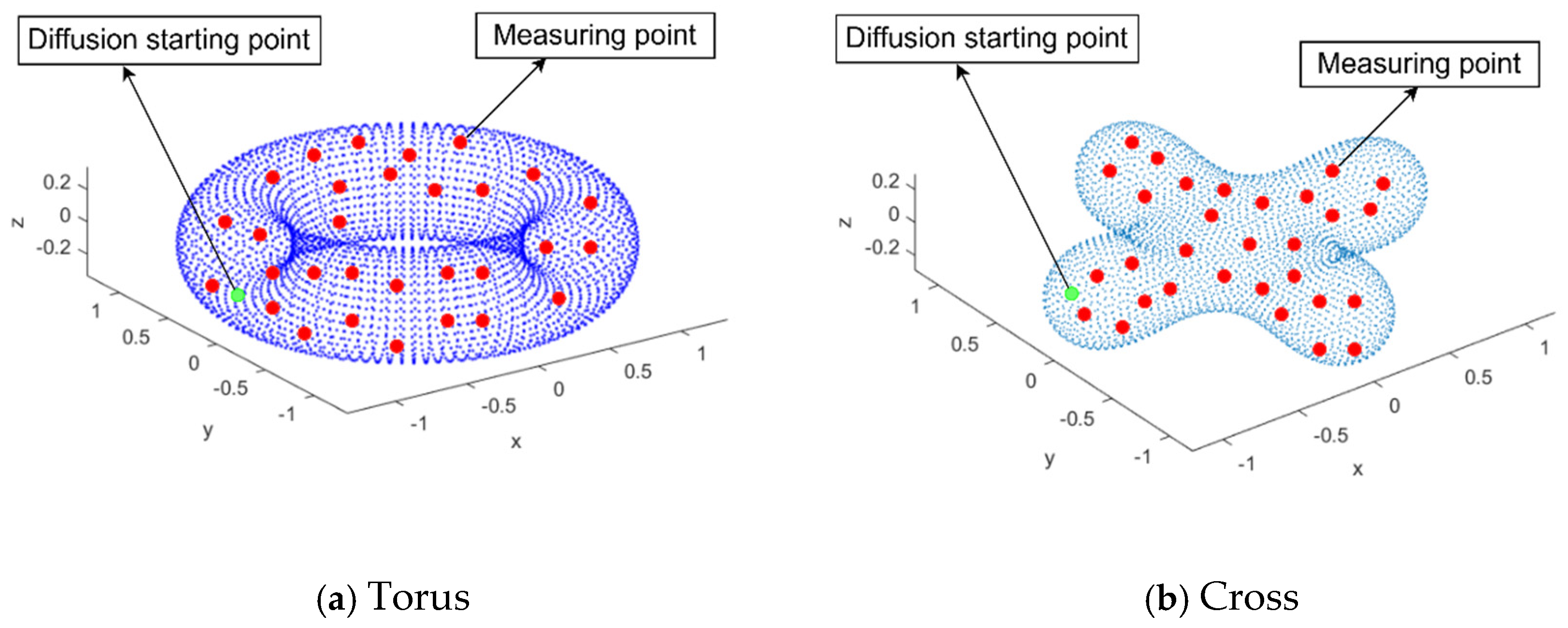
In this case, there is no analytical solution to the equation, and the GFDM approximation is used to invert diffusion coefficient D. A total of 30 points on the surface are ramdonly selected as observation points. The time step is 0.01 s. The simulated diffusion results corresponding to diffusion coefficient D at the observation point of 0.1 s is taken as the input feature X of the neural networks. Diffusion coefficient D is taken as output Y, so that a sample $\left(X,Y\right)$ can be constructed. For two different shapes, torus and cross, the number of samples for each shape training is 1000 sets of data. Each set of data contains the diffusion values of thirty detection points at different times. Then, 70% of the samples are divided into a study set and 30% of the samples are divided into verification sets to evaluate the generalization ability of the neural networks. The number of samples for testing is four sets of data, and the test set is not involved in the training of the neural networks. Figure 4 shows a schematic diagram of point sources and measuring points when the surface is torus and ellipsoid.

Table 4. Inversion results and errors of diffusion coefficients with torus surface.

${\mathit{D}}_{\mathit{t}\mathit{r}\mathit{u}\mathit{e}}$	${\mathit{D}}_{\mathit{p}\mathit{r}\mathit{e}\mathit{d}}$	$\mathit{E}$ (%)
1.5050	1.5042	0.05
2.5050	2.5181	0.66
3.5050	3.4826	0.50
4.5050	4.4961	0.20

and

Table 5. Inversion results and errors of diffusion coefficients with cross surface.

${\mathit{D}}_{\mathit{t}\mathit{r}\mathit{u}\mathit{e}}$	${\mathit{D}}_{\mathit{p}\mathit{r}\mathit{e}\mathit{d}}$	$\mathit{E}$ (%)
1.5050	1.5012	0.25
2.5050	2.4925	0.50
3.5050	3.4941	0.34
4.5050	4.5179	0.29

show the inversion results and errors of diffusion coefficients when the surface is torus and cross, respectively.

From Table 4 and Table 5, it can be observed that for different models, the predicted value of diffusion coefficient D is almost consistent with the actual value, and the error is in the order of $10^{-3}$. Therefore, the proposed model can achieve accurate inversion of diffusion coefficient D in the absence of an analytic solution.

• Example 3.

Based on the inversion of the diffusion coefficient and source term coefficient in the previous example, the diffusion coefficient and source term coefficient will be further inverted at the same time. Since the observed data in practical applications often contain noise (especially Gaussian noise), to verify the numerical performance of RBF neural networks under different noise levels, this paper adds Gaussian noise at different levels to the data, and the noise is added in the following way

$$u_{noise}=u+noise\cdot std\left(u\right)\cdot \epsilon ,\epsilon ~N\left(\mathrm{0,1}\right),$$

(25)

where $noise$ is noise level, $std\left(u\right)$ is the standard deviation of the whole observed dataset, $\epsilon$ is the probability density function, and $N\left(\mathrm{0,1}\right)$ is the standard normal distribution.

The fractional diffusion equation on a closed smooth surface in three dimensions is given as

$${\displaystyle \frac{{𝜕}^{\alpha }u\left(\mathbf{x},t\right)}{𝜕t^{\alpha }}}=D{\Delta }_{s}u\left(\mathbf{x},t\right)+Q\left(\mathbf{x},t\right),0<\alpha <1,x\in S,t\in \left(0,T\right),$$

(26)

where $D$ is the diffusion coefficient, $\alpha ={\displaystyle \frac{1}{2}}$, source term coefficient $Q\left(\mathbf{x},t\right)=d$, and the analytical solution is given as

$$u\left(t,\mathbf{x}\right)=x\cdot \left(x^4-10x^2{y}^2+5y^4\right)\cdot \left(x^2+y^2-60z^2\right)\cdot t.$$

(27)

There is no diffusion at the initial moment, and from the initial moment, all the cloth points on the surface of the entire surface begin to diffuse at the same time and the time step is 0.01 s. In the detection domain, different diffusion coefficients D and source term coefficients d are randomly generated. Then, 30 points on the surface are randomly selected as observation points. The simulated diffusion results corresponding to diffusion coefficient D and source term coefficient d at 0.1 s of the observation point are taken as the input feature X of the neural networks, and diffusion coefficient D and source term coefficient d are taken as the output Y. This allows you to construct a sample $\left(X,Y\right)$. For three different shapes, spherical surface, torus, and cross, the number of samples for each shape training is 1000 sets of data. Each set of data contains the diffusion values of thirty detection points at different times. Then, 70% of the samples are divided into a study set and 30% of the samples are divided into verification sets to evaluate the generalization ability of the neural networks. The number of samples for testing is six sets of data, and the test set is not involved in the training of the neural networks.

Table 6. Parameter coupling inversion errors when the surface is a sphere.

		Error Values at Different Noise Levels
		0%	1%	5%
Case 1	diffusion coefficient D	0.0123	0.0134	0.0144
	source term coefficient d	0.0207	0.0216	0.0225
Case 2	diffusion coefficient D	0.0231	0.0242	0.0250
	source term coefficient d	0.0247	0.0256	0.0265
Case 3	diffusion coefficient D	0.0244	0.0253	0.0260
	source term coefficient d	0.0157	0.0166	0.0175

,

Table 7. Parameter coupling inversion errors when the surface is torus.

		Error Values at Different Noise Levels
		0%	1%	5%
Case 1	diffusion coefficient D	0.0221	0.0230	0.0239
	source term coefficient d	0.0222	0.0231	0.0240
Case 2	diffusion coefficient D	0.0155	0.0164	0.0173
	source term coefficient d	0.0102	0.0111	0.0120
Case 3	diffusion coefficient D	0.0109	0.0118	0.0127
	source term coefficient d	0.0298	0.0307	0.0316

and

Table 8. Parameter coupling inversion errors when the surface is cross.

		Error Values at Different Noise Levels
		0%	1%	5%
Case 1	diffusion coefficient D	0.0179	0.0188	0.0197
	source term coefficient d	0.0182	0.0191	0.0200
Case 2	diffusion coefficient D	0.0125	0.0134	0.0143
	source term coefficient d	0.0251	0.0260	0.0269
Case 3	diffusion coefficient D	0.0262	0.0271	0.0280
	source term coefficient d	0.0287	0.0296	0.0305

show the inversion results and errors of diffusion coefficient D and source coefficient d when the surface is spherical, torus, and cross, respectively. The noise level considers interference with the inversion error at 0%, 1%, and 5%.

From Table 6, Table 7 and Table 8, it can be observed that for different models, the predicted values of the diffusion coefficient and source coefficient are almost consistent with the actual values, and the error is in the order of $10^{-2}$. Therefore, the proposed model can achieve joint inversion of the diffusion coefficient and source coefficient more accurately. At the same time, it can be noted that when the noise level increases, the inversion error will increase, but in an acceptable range.

• Example 4.

In this example, the diffusion coefficient and the fractional order will be inverted at the same time. The fractional diffusion equation on a closed smooth surface in three dimensions is defined as Equation (26), where $D$ is the diffusion coefficient, $\alpha ={\displaystyle \frac{1}{2}}$, source term coefficient $Q\left(\mathit{x},t\right)=0$, and the analytical solution is given as Equation (27).

The time step is 0.01 s. In the detection domain, different diffusion coefficients D and fractional orders $\alpha$ are randomly generated. Then, 30 points on the surface are randomly selected as observation points. The simulated diffusion results corresponding to diffusion coefficient D and fractional order $\alpha$ at 0.1 s of the observation point are taken as the input feature X of the neural networks, and diffusion coefficient D and fractional order $\alpha$ are taken as the output Y. This allows you to construct a sample $\left(X,Y\right)$. For two different shapes, spherical surface and torus, the number of samples for each shape training is 1000 sets of data. Each set of data contains the diffusion values of thirty detection points at different times. Then, 70% of the samples are divided into a study set and 30% of the samples are divided into verification sets to evaluate the generalization ability of the neural networks. The number of samples for testing is six sets of data, and the test set is not involved in the training of the neural networks.

Table 9. Parameter coupling inversion errors when the surface is a sphere.

		True Value	Predicted Value	Error Value (%)
Case 1	diffusion coefficient D	0.6500	0.6534	0.5231
	fractional order $\alpha$	0.1500	0.1528	1.8667
Case 2	diffusion coefficient D	0.7500	0.7542	0.5600
	fractional order $\alpha$	0.2500	0.2568	2.7200
Case 3	diffusion coefficient D	0.8500	0.8553	0.6235
	fractional order $\alpha$	0.3500	0.3438	1.7714

and

Table 10. Parameter coupling inversion errors when the surface is a torus.

		True Value	Predicted Value	Error Value (%)
Case 1	diffusion coefficient D	0.6500	0.6513	0.2000
	fractional order $\alpha$	0.1500	0.1571	4.7333
Case 2	diffusion coefficient D	0.7500	0.7553	0.7067
	fractional order $\alpha$	0.2500	0.2543	1.7200
Case 3	diffusion coefficient D	0.8500	0.8535	0.4118
	fractional order $\alpha$	0.3500	0.3340	4.5714

show the inversion results and errors of diffusion coefficient D and fractional order $\alpha$ when the surface is spherical and torus, respectively.

From Table 9 and Table 10, it can be observed that for different models, the predicted values of the diffusion coefficient and fractional order are almost consistent with the actual values, and the error is in the order of $10^{-2}$. Therefore, the proposed model can achieve joint inversion of the diffusion coefficient and fractional order more accurately. Furthermore, the numerical results obtained in these examples clearly demonstrate that RBF neural networks can invert the parameters of the diffusion equation with high accuracy. The hybrid method based on the GFDM and RBF neural networks can accurately invert the parameters even if there is an analytic solution of the equation.

In fact, during the input of training samples, the inversion result is relatively accurate only when the diffusion coefficient and the order increase or decrease concurrently. If the diffusion coefficient and the order change irregularly, it is very difficult to accurately invert the sought-after result. In order to obtain the result accurately when the desired parameter changes irregularly, it may be necessary to introduce a more advanced neural grid, such as PINNs.

5. Conclusions

This paper delves into the inverse problems of anomalous diffusion on the surface. For the inverse problems, RBF neural networks are primarily utilized to invert the relevant parameters of anomalous diffusion on the surface. The GFDM is primarily employed to discretely solve the fractional derivative model on the surface. The training database for RBF neural networks to inverse the desired parameters is established by solving the proposed time-fractional diffusion equation using the GFDM.

The results of the four examples show that the hybrid method can obtain the required parameters quickly and accurately under different conditions. For GFDM, RMSE results show that GFDM has the advantage of high calculation accuracy. And, because of the factors of GFDM itself, it is more simplified and the calculation time is shorter than other methods. For RBF neural networks, the inversion results show that it has high precision in the inversion of different problems. And, because of the factor of RBF neural networks itself, the inversion time of RBF neural networks is shorter than that of other methods.

For future research, there is a lack of studies on non-smooth, non-closed, and asymmetrical surface models in this field, which warrants further investigation. In this paper, we introduced the time-fractional model to define the anomalous diffusion problem on the surface. However, other models, such as the space fractional derivative model or the space-time fractional derivative model, can also be used to describe anomalous diffusion on the surface.