Article

Mathematical Modeling and Analysis of Tumor Growth Models Integrating Treatment Therapy

1
Division of Science and Technology, Department of Mathematics, University of Education Lahore, Lahore 54770, Pakistan
2
Oral & Maxillofacial Radiology, School of Dental Sciences, Health Campus, Universiti Sains Malaysia, Kota Bharu 16150, Malaysia
3
Dental Research Unit, Center for Transdisciplinary Research (CFTR), Saveetha Institute of Medical and Technical Sciences, Saveetha Dental College, Saveetha University, Chennai 602105, India
4
Biomedical Sciences Programme, School of Postgraduate, YARSI University, Jakarta 10510, Indonesia
*
Author to whom correspondence should be addressed.
Math. Comput. Appl. 2025, 30(6), 119; https://doi.org/10.3390/mca30060119
Submission received: 9 September 2025 / Revised: 22 October 2025 / Accepted: 25 October 2025 / Published: 30 October 2025
(This article belongs to the Special Issue Feature Papers in Mathematical and Computational Applications 2025)

Abstract

This study presents a comparative analysis of tumor growth models based on logistic, exponential, and Gompertz formulations. Their response to therapeutic intervention is examined to identify which model shows better behavior with minimal decline of immune cells. The framework incorporates three main cell populations as follows: natural killer cells, cytotoxic T cells, and tumor cells, along with treatment effects. Dynamical properties such as positive invariance, existence, boundedness, and equilibrium stability are investigated. Numerical simulations indicate that the logistic model gives more favorable treatment outcomes compared to the exponential and Gompertz models. The results also show a faster decline of immune cell populations in the exponential and Gompertz models than in the logistic model under varying drug flux.

1. Introduction

Cancer comes from the Greek word karkinos, meaning crab. It was first reported in the 1600s and is defined as the abnormal growth of cells that can invade and spread to other parts of the body [1]. Tumor is a fatal disease and is the second leading cause of mortality worldwide [2,3]. Tumors are classified as benign or malignant, as shown in Table 1. Figure 1 shows MRI images of a tumor.
In recent years, mathematical oncology has developed many models to study cancer dynamics. These models provide a theoretical framework for exploring immune-oncological pathways [4,5]. They allow the study of immune system dynamics, tumor behavior, treatment strategies, and the prediction of outcomes of new therapies [6,7,8,9,10]. Mathur [11] explored how mathematical models can guide treatment beyond standard regimens. Yin et al. [12] reviewed models addressing solid tumor dynamics and drug resistance. Their work supports model-based approaches for analyzing treatment response and resistance. The authors in [13] provided a model to measure the hormesis of anti-tumor drugs and identify the critical antibody dose. Lopez et al. [14] developed a model that includes tumor, healthy host cells, and immune effector cells. Abernathy [15] studied oncolytic virotherapy using a logistic growth model. Bao et al. [16] analyzed the effects of immunotherapy and chemotherapy, showing that combination therapy is necessary for complete tumor removal. Claret et al. [17] developed a tumor growth inhibition model that links drug exposure with tumor size data and survival outcomes. Unni et al. [18] proposed a model that integrates therapy and immune interactions involving dendritic cells, natural killer cells, and cytotoxic T cells. Azizi et al. [19] summarized the key applications of mathematical modeling in oncology, including immunology, heterogeneity, personalized therapy, tumor progression, and trial optimization. Magni and Lavezzi et al. [20,21] reviewed tumor progression models and their role in laboratory and animal studies. Poggesi et al. [22] developed an ODE-based model to describe cancer growth in xenograft studies. Pang et al. [6] analyzed tumor behavior using standard models and found chemotherapy to be effective in reducing tumor cells. Mishra et al. [23] used a fractional model to study chemotherapy effects on both tumor and normal cells. Their results showed that regular drug dosing can suppress tumor growth. Bunonyo et al. [24] studied exponential tumor growth with combined therapy and concluded that multi-treatment strategies are more effective. Tosca et al. [25] applied a PK–TGI model to support dose selection in early trials. Rocchetti and Simeoni et al. [26,27] proposed PK-PD models to study tumor response under cytostatic therapy. Butner et al. [28] developed a model and used it to study the tumor growth and immune response parameters to stratify patients on long-term tumor burden. Pang [29] designed an immune response model with bifurcations. Valle et al. [30] created a six-dimensional model to explain tumor evolution under therapy. Ronchi et al. [31] built a framework to estimate tumor doubling time and survival curves from xenograft data. Raeisi et al. [32] studied colon cancer spread using a mathematical model. Makhlouf et al. [33] modeled interactions between tumor cells, NK cells, CD4+, CD8+ T cells, and circulating lymphocytes under therapy.
The tumor growth law fundamentally determines model stability, tumor progression, and treatment response. Logistic, exponential, and Gompertz formulations represent distinct biological behaviors—bounded and stable growth, unrestricted and unstable proliferation, and decelerating yet parameter-sensitive expansion, respectively [14,18,24,29]. Therefore, choosing an appropriate growth model is vital for accurately predicting tumor dynamics and optimizing therapeutic strategies.
The novelty of this work is a unified framework that integrates the following three tumor growth laws: logistic, Gompertz, and exponential combined with NK and CTL immune responses under chemotherapy. Unlike studies limited to single models, this work compares therapeutic outcomes across models. The results show that the logistic model suppresses tumors while better preserving immune cells. This comparative approach provides new insights and supports the design of improved therapy strategies. The framework considers NK cells, CTLs, and tumor cells and studies their response to treatment. Dynamical properties, including stability, existence, boundedness, and invariance are analyzed. The model is solved numerically using the Runge–Kutta method Python 3.11 .
This paper has seven sections. Section 1 is the introduction. Section 2 presents tumor growth models and their formulations. Section 3 describes the combined model. Section 4 and Section 5 explain the system dynamics, including boundedness, existence, invariance, and stability. Section 6 presents the results and discussion. Section 7 presents some concluding remarks.

2. Mathematical Models of Tumor Growth

2.1. Tumor Growth Models

Several growth functions have been studied in epidemiology and ecology. First-order ordinary differential equations are widely used to predict tumor growth by describing changes in tumor volume over time. The most common formulations are exponential and logistic models [34,35].

2.1.1. Exponential Models

  • Malthusian Model: d T d t = c T ,   c > 0 , T is tumor volume in m 3 and c is growth rate in m 3 day 1 .
  • Power Law Model: d T d t = c T m ,   c > 0 ,   m > 0 , and m is a real constant.
  • Migration Model: d T d t = c T + K ,   c > 0 ,   K > 0 , where K is the migration rate.
  • Gompertz Model: d T d t = α e b t T ,   α > 0 ,   b > 0 , where α is the intrinsic growth parameter and b is the parameter of growth deceleration.

2.1.2. Generalized Logistic Model

The generalized form of the logistic equation is as follows [35]:
d T d t = p T m 1 T K δ λ ,
where m, δ , and λ are nonnegative exponents and p is the tumor growth rate in m 3 day 1 . From Equation (1), we can deduce all forms of models as follows: The above equation turns into an exponential equation for m = 1 and λ = 0 as
d T d t = p T .
The logistic model can be obtained by putting m = δ = λ = 1 in Equation (1) as,
d T d t = p T 1 T K ,
and for m = 2 / 3 , δ = 1 / 3 , and λ = 1 we have a Von Bertalanffy equation model expressed as,
d T d t = p T 2 / 3 1 T K 1 / 3 .
where p is the growth rate and q is the growth deceleration parameter. Equation (1) expresses Richard’s model for m = 1 and λ = 1 as
d T d t = p T 1 T K δ .

3. Formulation of the Mathematical Model

The key parameters and their biological interpretation are outlined as follows:
  • ℵ: Natural killer cells: provide an immediate, nonspecific anti-tumor defense.
  • Ł: Cytotoxic T lymphocytes: delayed, specific immune response that strengthens and sustains tumor clearance after activation.
  • τ : Tumor cells.
  • a 1 τ ( 1 a 2 τ ) : Tumor proliferation.
  • a 3 τ : Immune-mediated tumor killing by NK cells.
  • β 1 τ Ł : Immune-mediated tumor killing by CTL.
  • b τ τ C : Drug-induced cytotoxicity.
  • b C : Drug-related immune cell death.
  • b Ł Ł C : Drug-related immune cell death.
  • w Ł ,   ρ : Natural death of CTL and NK cells.
  • r τ : Immune cell activation.
This study considers three tumor models that involve three cell populations as follows: tumor cells τ ( t ) , natural killer (NK) cells ( t ) , and cytotoxic T cells Ł ( t ) . Their dynamics are described under the influence of chemotherapy drug concentration C ( t ) . Each cell population is modeled using an ordinary differential equation of the following form [18]:
d [ . ] d t = P ( . ) Q ( . ) K [ . ] [ . ] .
where P [ . ] and Q [ . ] represent proliferation, competition, and inhibition functions, and K [ . ] describes the effect of chemotherapy. It is assumed that natural killer cells grow logistically through the term a 4 ( 1 a 5 ) , where a 4 and a 5 express the growth rate and reciprocal of the carrying capacity, respectively. Additionally, natural killer cells are influenced by the interaction of NK cells and tumor cells [35] denoted by a 6 τ and the interaction with the drug by b C . Also, the inactivation or natural death of NK cells has been denoted by ρ . Here, the parameters a 6 , ρ , and b express death of NK cells by tumor, natural death of NK cells, and death of NK cells by the drug, respectively. Thus, the differential equation describing the dynamics of NK cells is as follows:
d ( t ) d t = a 4 ( 1 a 5 ) a 6 τ ( t ) ( t ) ρ ( t ) b ( t ) C ( t ) .
Cytotoxic (CD8+ T) cells play a crucial role in the immune system’s ability to eliminate tumor cells. Tumor-specific CD8+ T lymphocytes are active while tumor cells are present but become inactive after some encounters [36,37]. They are recruited by tumor cells in a linear fashion as r τ . The cytotoxic cell population impacted by the interactions of cytotoxic cells with the tumor and drug are expressed by the terms β 2 τ Ł and b Ł Ł C ( t ) , respectively. Moreover the natural death of cytotoxic cells is represented by the term w Ł . Here, r, β 2 , b Ł , and w represents the activation rate of CD8+ cells, death of CD8+ by the tumor, death of CD8+ by drug, and natural death of CD8+ cells, respectively. Thus the dynamical equation of CD8+ cells is as follows:
d Ł ( t ) d t = r τ ( t ) ( t ) w Ł ( t ) β 2 τ ( t ) Ł ( t ) b Ł Ł C ( t ) .
It is supposed that tumor grows through a logistic function a 1 τ ( 1 a 2 τ ) . Here, parameters a 1 and a 2 represents the per capita growth rate and the inverse of tumor capacity [38]. The tumor growth has been impacted by the interactions of natural killer cells represented by a 3 τ , cytotoxic cells β 1 τ Ł , and therapy b τ τ C ( t ) [36,39]. Where a 3 , β 1 , and b τ describe tumor death by natural killer cells, tumor death by cytotoxic cells, and tumor cell death by the drug, respectively. Thus, tumor dynamics can be expressed as
d τ ( t ) d t = a 1 τ ( 1 a 2 τ ) a 3 τ ( t ) ( t ) β 1 τ ( t ) Ł ( t ) b τ τ ( t ) C ( t ) .
The dynamical equation expressing chemotherapy drug intervention is
d C d t = κ C o C ( t ) .
where κ and C o describe chemotherapy drug influx and drug decay, respectively. Table 2 lists the parameters and their dimensions.
Thus, the complete logistic model is
d ( t ) d t = a 4 ( t ) ( 1 a 5 ( t ) ) a 6 τ ( t ) ( t ) ρ ( t ) b ( t ) C ( t ) , d Ł ( t ) d t = r τ ( t ) ( t ) w Ł ( t ) β 2 τ ( t ) Ł ( t ) b Ł Ł ( t ) C ( t ) , d τ ( t ) d t = a 1 τ ( t ) ( 1 a 2 τ ( t ) ) a 3 τ ( t ) ( t ) β 1 τ ( t ) Ł ( t ) b τ τ ( t ) C ( t ) , d C d t = κ C o C ( t ) .
with initial conditions τ ( 0 ) = τ 0 0 , ( 0 ) = 0 0 , Ł ( 0 ) = Ł 0 0 , and C ( 0 ) = c 0 0 .

4. Dynamics

4.1. Positive Invariance

We check positive invariance by analyzing the vector field on the system boundaries. Each variable is set to zero to see if the flow points inward or is tangent.
For ( t ) = 0 ,
d ( t ) d t | = 0 = a 4 ( 0 ) ( 1 a 5 ( 0 ) ) a 6 τ ( t ) ( 0 ) ρ ( 0 ) b ( 0 ) C ( t ) , = 0 at = 0 ,
Thus, no flow leaves through = 0 .
For Ł ( t ) = 0 ,
d Ł ( t ) d t | Ł = 0 = r τ ( t ) ( t ) w ( 0 ) β 2 τ ( t ) ( 0 ) b Ł ( 0 ) C ( t ) , Ł = r τ 0 ,
Since r , τ , 0 , the flow is nonnegative. No flow leaves through Ł = 0 . For τ = 0 ,
d τ ( t ) d t | τ = 0 = a 1 ( 0 ) ( 1 a 2 ( 0 ) ) a 3 ( 0 ) ( t ) β 1 ( 0 ) Ł ( t ) b τ ( 0 ) C ( t ) = 0 .
So, τ = 0 , and no flow leaves through τ = 0 .
Similarly, for C = 0 ,
d C d t | C = 0 = κ C 0 ( 0 ) = 0 , κ 0 ,
The flow is positive at C = 0 . So no outflow occurs. Since all derivatives on the boundaries are nonnegative, the vector field points inward or is tangent. Therefore, the positive orthant is invariant.

4.2. Boundedness

To show boundedness, define
V = + Ł + τ + C ,
and compute its time derivative along the system trajectories. First we will compute d V d t as follows:
d V d t = d d t + d Ł d t + d τ d t + d C d t .
Using the system (11) and Equation (8), we have
d V d t = a 4 ( t ) ( 1 a 5 ( t ) ) a 6 τ ( t ) ( t ) ρ ( t ) b ( t ) C ( t ) + r τ ( t ) ( t ) w Ł ( t ) β 2 τ ( t ) Ł ( t ) b Ł Ł ( t ) C ( t ) + a 1 τ ( t ) ( 1 a 2 τ ( t ) ) a 3 τ ( t ) ( t ) β 1 τ ( t ) Ł ( t ) b τ τ ( t ) C ( t ) + κ C o C ( t ) .
Arranging the terms by variables and signs, we have
d V d t = a 4 a 4 a 5 2 a 6 τ ρ b C + r τ w Ł β 2 τ Ł b Ł Ł C + a 1 τ a 1 a 2 τ 2 a 3 τ β 1 τ Ł b τ τ C + κ C 0 C .
By analyzing the signs of terms in the above equation, we have
  • Negative quadratic terms: a 4 a 5 2 and a 1 a 3 τ 2 help to control growth.
  • Negative linear terms: ρ ,   w Ł , and C 0 C provide damping.
  • Mixed terms are negative or zero as variables are nonnegative.
  • a 4 ,   r τ ,   a 1 τ , and κ are positive terms.
For greater values of , Ł , τ , and C , negative quadratic and linear terms dominate positive linear terms, implying that if V > M , for M > 0 , then V < 0 . Hence, solutions enter and remain in a bounded set.

4.3. Existence

Consider the system
d ( t ) d t = a 4 ( t ) ( 1 a 5 ( t ) ) a 6 τ ( t ) ( t ) ρ ( t ) b ( t ) C ( t ) , d Ł ( t ) d t = r τ ( t ) ( t ) w Ł ( t ) β 2 τ ( t ) Ł ( t ) b Ł Ł ( t ) C ( t ) , d τ ( t ) d t = a 1 τ ( t ) ( 1 a 2 τ ( t ) ) a 3 τ ( t ) ( t ) β 1 τ ( t ) Ł ( t ) b τ τ ( t ) C ( t ) , d C d t = κ C o C ( t ) .
with initial conditions τ ( 0 ) = τ 0 0 , ( 0 ) = 0 0 , Ł ( 0 ) = Ł 0 0 , and C ( 0 ) = c 0 0 .
Now define the system in vector form as follows: x ( t ) = [ ( t ) , ( t ) , τ ( t ) , C ( t ) ] T . Thus, we have,
d x d t = f ( t , x ) .
Since each component of the function is a polynomial in x, all expressions are continuous in all variables. Also, these expressions are polynomial or rational functions so they are differentiable functions.
A function is Lipschitz continuous if the following holds:
f ( t , x ) f ( t , y ) L x y ,
Now the Jacobian matrix of model (11) at a general point is
J = a 4 2 a 4 a 5 a 6 τ ρ C 0 a 6 r τ w β 2 τ C r β 2 Ł Ł a 3 τ β 1 τ a 1 2 a 1 a 2 τ a 3 β 1 Ł C τ 0 0 0 C 0 ,
From above, we can see that all partial derivatives are continuous and bounded on any compact subset. Thus, f ( t , x ) is locally Lipschitz in x. Hence, the initial value problem has a unique local solution in some interval [ 0 , T ] , for some T > 0 .

5. Stability Analysis

For nonlinear systems, stability is studied around equilibrium points. The system is first linearized, and the Jacobian matrix is computed. Eigenvalues of the Jacobian determine stability. The Routh–Hurwitz theorem is applied for higher-order cases. The Jacobian of system (11) at a general point is
J = a 4 2 a 4 a 5 a 6 τ ρ C 0 a 6 r τ w β 2 τ C r β 2 Ł Ł a 3 τ β 1 τ a 1 2 a 1 a 2 τ a 3 β 1 Ł C τ 0 0 0 C 0 ,
Equilibrium points are obtained by setting τ = Ł = = C = 0 .
a 4 ( t ) ( 1 a 5 ( t ) ) a 6 τ ( t ) ( t ) ρ ( t ) b ( t ) C ( t ) = 0 , r τ ( t ) ( t ) w Ł ( t ) β 2 τ ( t ) Ł ( t ) b Ł Ł ( t ) C ( t ) = 0 , a 1 τ ( t ) ( 1 a 2 τ ( t ) ) a 3 τ ( t ) ( t ) β 1 τ ( t ) Ł ( t ) b τ τ ( t ) C ( t ) = 0 , κ C o C ( t ) = 0 .
This implies the following:
= a 4 a 6 τ ρ C a 4 a 5 = a 4 a 6 τ ρ κ C 0 a 4 a 5 , where , C = κ C o , Ł = r τ w + C + β 2 τ
and
τ = a 1 a 3 β 1 Ł C a 1 a 2 .
Three cases are identified as follows:
  • ( I ) . (Steady State or dead state) All populations (tumor and immune cells) go to zero, i.e., = Ł = τ = 0 . This represents a biologically unrealistic outcome but mathematically corresponds to system extinction. So, the equilibrium point is E 0 ( 0 , 0 , 0 , κ C o ) .
The Jacobian matrix of Equation (11) at point E 0 is
J ( E 0 ) = a 4 ρ κ C o 0 0 0 0 w κ C o 0 0 0 0 a 1 κ C o 0 0 0 0 C o ,
The eigenvalues of J ( E 0 ) are λ 1 = a 4 ρ κ C o , λ 2 = w κ C o , λ 3 = a 1 κ C o , and λ 4 = C o , From here, we conclude that E 0 is locally asymptotically stable if λ 1 < 0 and λ 3 < 0 , i.e., κ > C o ( a 4 ρ ) or κ > a 1 C o . , and E 0 is unstable if κ = C o a 1 or κ = C o ( a 4 ρ ) and is stable for κ > m a x { a 1 C o , C o ( a 4 ρ ) } .
Thus, the following stability results can be obtained.
  • E 0 will be locally stable if κ > m a x { a 1 C o , C o ( a 4 ρ ) } .
  • E 0 is unstable if κ = C o a 1 or κ = C o ( a 4 ρ ) .
  • ( I I ) . (Tumor-free state) Tumor cells vanish, i.e., τ = 0 , while immune cells and possibly drug concentration settle at positive levels. This indicates successful therapy or immune clearance, where the body eliminates cancer and maintains immune activity. So, the equilibrium point is E 1 a 4 ρ κ C o a 4 a 5 , 0 , 0 , κ C o and the Jacobian matrix of Equation (11) at the E 1 point is
    J ( E 1 ) = a 4 ρ κ C o 0 a 6 a 4 ρ κ C o a 4 a 5 0 0 w κ C o r a 4 ρ κ C o a 4 a 5 0 0 0 a 1 a 3 a 4 ρ κ C o a 4 a 5 κ C o 0 0 0 0 C o ,
    The eigenvalues of J ( E 1 ) are λ 5 = a 4 ρ κ C o , λ 6 = w κ C o , λ 7 = a 1 a 3 a 4 ρ κ C o a 4 a 5 , and λ 8 = C o . For the tumor-free state, λ 5 and λ 7 must be negative, so from the above expressions a 4 > ρ κ C o ; thus, λ 5 < 0 , and for λ 7 < 0 we must have κ > ( a 1 a 4 a 5 a 3 a 4 + a 3 ρ ) C o a 4 a 5 a 3 .
Using the Routh–Hurwitz theorem [40] the following conditions of stability are obtained.
  • E 1 is stable if λ 5 < 0 , λ 7 < 0 , i.e., for κ > ( a 1 a 4 a 5 a 3 a 4 + a 3 ρ ) C o a 4 a 5 a 3 .
  • E 1 is unstable if κ = ( a 1 a 4 a 5 a 3 a 4 + a 3 ρ ) C o a 4 a 5 a 3 .
  • ( I I I ) . (Tumor-present state) Tumor persists at a positive equilibrium along with immune cells (NK and CTLs) and drug concentration. This reflects a chronic or controlled tumor burden, where the cancer is not eradicated but stabilized under immune and drug pressure. Thus, the equilibrium point becomes as follows: E 2 0 , 0 , a 1 κ C o a 1 a 2 , κ C o . So the Jacobian matrix of Equation (11) at E 2 is
    J ( E 2 ) = a 1 ρ κ C o a 6 Λ 0 0 0 r Λ w κ C o β 2 Λ 0 0 a 3 Λ β 1 Λ a 1 2 a 1 a 2 Λ κ C o Λ 0 0 0 C o ,
    where Λ = a 1 κ C o a 1 a 2 . The eigenvalues of J ( E 2 ) are λ 9 = a 1 ρ κ C o a 6 Λ , λ 10 = w κ C o β 2 Λ , λ 11 = a 1 2 a 1 a 2 Λ κ C o . For the tumor-present state to be locally stable, λ 9 & λ 11 should be negative. After simplifying the expressions of λ 9 and λ 11 , one can have a 1 ρ κ C o < 0 . So λ 9 < 0 . When a 1 κ C o ρ > 0 and λ 9 < 0 , we have κ > ( a 1 a 2 ( a 1 ρ ) a 1 a 6 ) C o a 1 a 2 a 6 .
The stability results indicate that when the drug influx rate κ exceeds the combined thresholds of tumor growth a 1 and immune activation parameters, the system reaches a stable tumor-free equilibrium, representing tumor elimination with preserved immune activity. Conversely, insufficient drug influx or high decay C o leads to a stable tumor-present state, corresponding to therapeutic failure or residual disease. Clinically, this reflects that optimizing chemotherapy dosage and immune-related parameters such as NK cell growth a 4 and cytotoxic activity β 1 is critical for maintaining long-term tumor control and preventing immune exhaustion.
Now, assume that the tumor and natural killer cells follow exponential growth. Thus, the mathematical model of exponential growth is expressed as follows:
d ( t ) d t = a 4 ( t ) a 6 τ ( t ) ( t ) ρ ( t ) b ( t ) C ( t ) , d Ł ( t ) d t = r τ ( t ) ( t ) w Ł ( t ) β 2 τ ( t ) Ł ( t ) b Ł Ł ( t ) C ( t ) , d τ ( t ) d t = a 1 τ ( t ) a 3 τ ( t ) ( t ) β 1 τ ( t ) Ł ( t ) b τ τ ( t ) C ( t ) , d C d t = κ C o C ( t ) .
with initial conditions τ ( 0 ) = τ 0 0 , ( 0 ) = 0 0 , Ł ( 0 ) = Ł 0 0 , and C ( 0 ) = c 0 0 .
The tumor model of Gompertz growth is expressed as follows:
d ( t ) d t = a 4 ( t ) e a 5 t a 6 τ ( t ) ( t ) ρ ( t ) b ( t ) C ( t ) , d Ł ( t ) d t = r τ ( t ) ( t ) w Ł ( t ) β 2 τ ( t ) Ł ( t ) b Ł Ł ( t ) C ( t ) , d τ ( t ) d t = a 1 τ ( t ) e a 2 t a 3 τ ( t ) ( t ) β 1 τ ( t ) Ł ( t ) b τ τ ( t ) C ( t ) , d C d t = κ C o C ( t ) .
with initial conditions τ ( 0 ) = τ 0 0 , ( 0 ) = 0 0 , Ł ( 0 ) = Ł 0 0 , and C ( 0 ) = c 0 0 . The formulation of tumor growth dynamics markedly determines the pattern and stability of equilibrium states in tumor–immune–drug systems. The logistic framework, constrained by a carrying capacity, portrays limited proliferation and typically yields stable tumor-free or controlled equilibria when treatment efficacy is adequate [14,18]. Conversely, the exponential representation implies unrestricted growth potential, often resulting in unstable or unbounded tumor expansion unless counteracted by intensive therapeutic intervention [24,29]. The Gompertz formulation, characterized by the gradual slowing of growth with tumor enlargement, exhibits intermediate stability that can fluctuate with therapeutic strength [15]. Collectively, logistic growth tends to promote more stable and biologically realistic control outcomes, whereas exponential and Gompertz laws describe faster or treatment-sensitive tumor progression.
The stability analysis of the tumor–immune–chemotherapy model reveals that its long-term dynamics are primarily governed by the chemotherapy drug influx and decay rates. Tumor-free equilibrium stability is achieved when the influx rate surpasses a threshold defined by the tumor growth and immune response parameters, leading to tumor elimination and sustained immune activity. When this condition is not satisfied, the system tends toward a tumor-present equilibrium, signifying treatment inefficacy or tumor persistence. Immune-related parameters, including natural killer cell proliferation and death rates, also affect the system’s capacity to maintain immune surveillance. Overall, the analysis underscores the necessity of optimizing treatment parameters to balance tumor suppression and immune preservation, providing a foundation for effective chemotherapy design and scheduling.

6. Results and Discussion

This section presents the numerical results of the proposed models using the Runge–Kutta method. The initial populations of tumor cells, natural killer cells, cytotoxic T cells, and the drug are assumed to be 20, 50, 30, and 5, respectively, over a time span of 100 days.
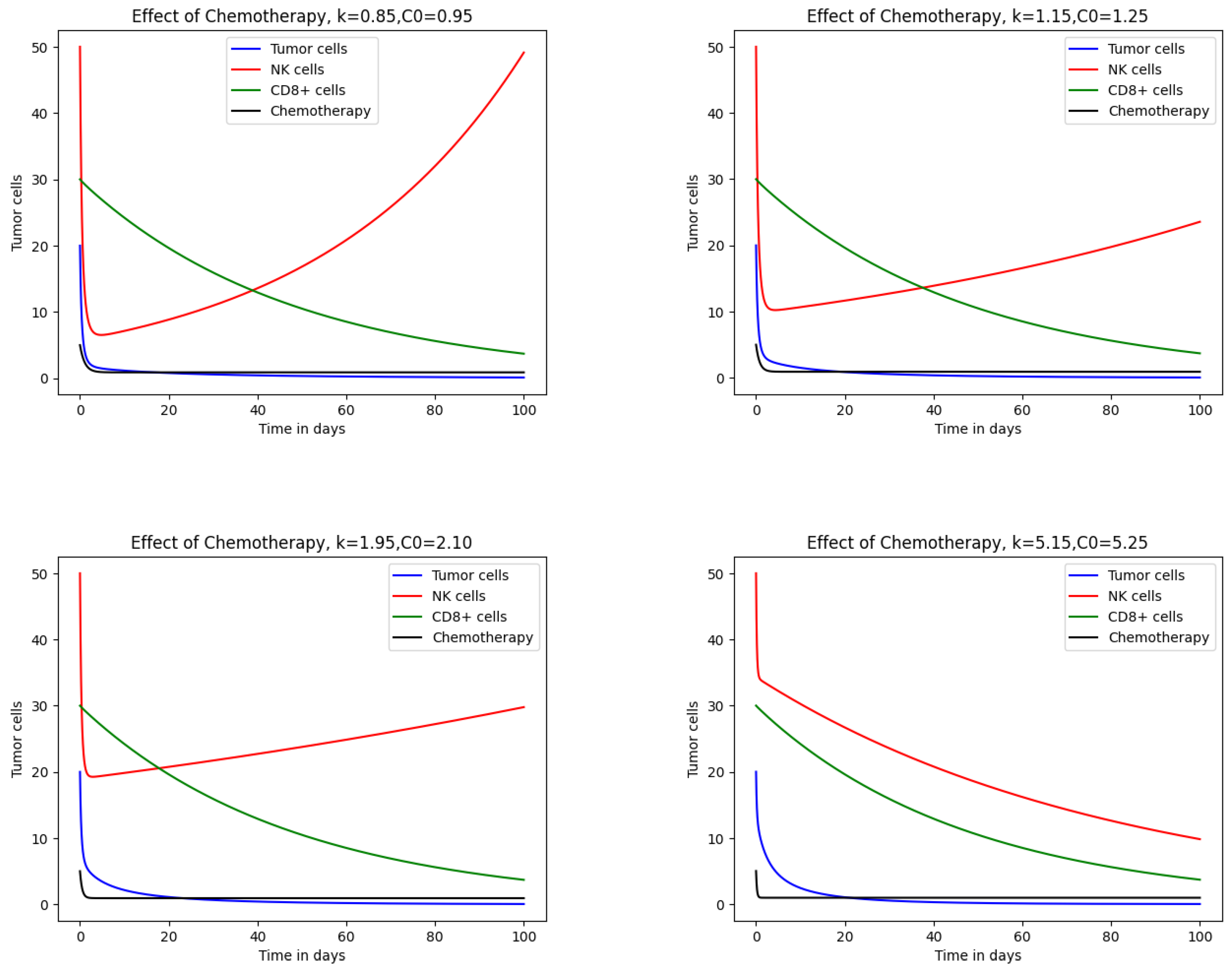
Figure 2 illustrates the effect of chemotherapy on different cell populations, including NK and tumor cells exhibiting logistic growth, keeping all other parameters fixed. In the first case, with drug concentration κ = 0.85 and decay rate C o = 0.95 , the tumor population decreases rapidly. NK cells initially decline but later recover, suggesting that the immune response is not significantly weakened and the patient has significant immune strength against the tumor. The second case, with κ increased to 1.15 and C o = 1.25 , shows further tumor reduction while healthy cells remain largely unaffected, which indicates a preserved immune system. In the third case, with κ = 1.95 and C o = 2.10 , the tumor continues to regress while only limited damage is observed in healthy cells, indicating that the immune system has been adjusted with drug concentration. When κ increases to 5.15 , the results indicate a sharp decline in the NK and CTL populations, reflecting the adverse effects of drugs on the immune system.
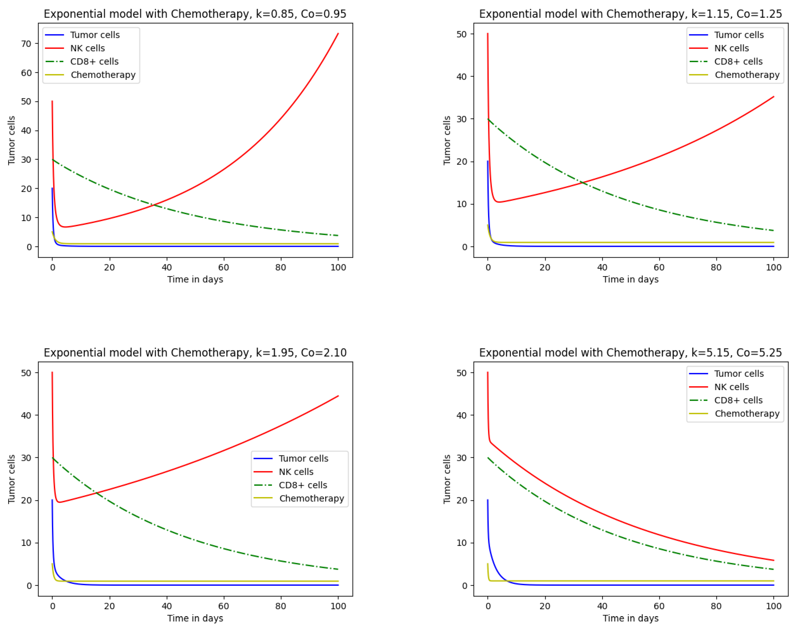
Figure 3 presents the effect of chemotherapeutic drugs on cell populations under exponential growth. Tumor and immune cell dynamics were examined for κ = 0.85 , 1.15 , 1.90 , and 5.15 with decay rates C o = 0.75 , 1.25 , 2.10 , and 5.35 , respectively. In the first case, with κ = 0.85 and C o = 0.95 , tumor cells are completely eliminated while natural cells remain unaffected. NK cells decline initially but later recover due to drug influx. Such a situation is unlikely because realistically, at the initial stage, the whole tumor has been eradicated. Although tumor cells are eliminated, the treatment also affects healthy cells. At higher values, such as κ = 5.15 , both tumor and immune cell populations decrease sharply. In severe cases, NK cells are entirely eliminated, indicating host mortality. Increasing κ from 0.85 to 1.15 , 1.90 , and 5.15 produces marked changes in tumor and immune cell behavior, as shown in Figure 2 and Figure 3, where κ = 5.15 and C 0 = 5.35 . These results demonstrate that chemotherapy consistently destroys tumor cells but also damages healthy cells. A comparison of Figure 2 and Figure 3 shows that drug effects on healthy cells are less pronounced under logistic growth, while exponential growth leads to greater impairment. Thus, the logistic growth model yields more favorable outcomes than exponential growth for the same parameter values.
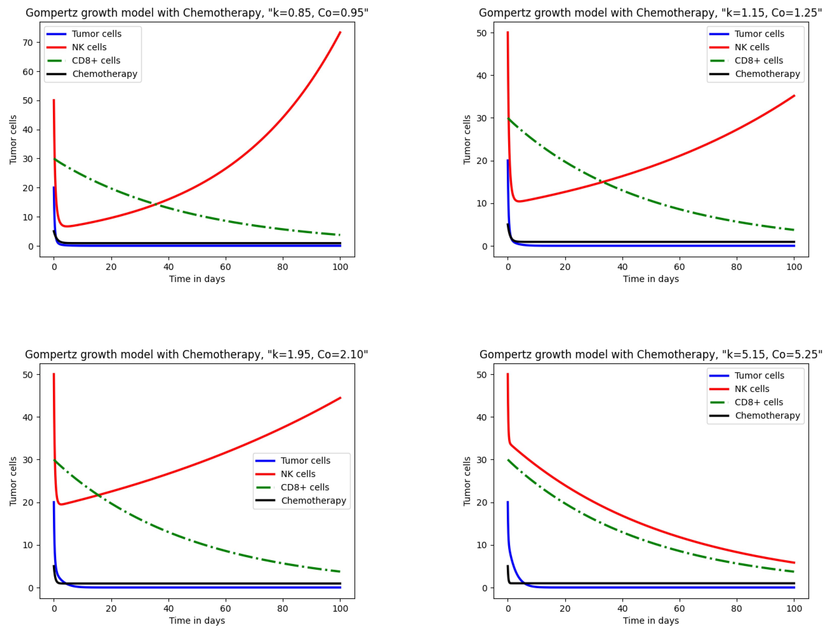
Figure 4 presents the response of tumor cells, NK cells following Gompertz growth, and CTLs described in model (18) under chemotherapy. At lower drug influx and decay rates, tumor and CTL cells show a behavior similar to that in the logistic and exponential models. As κ increases from 0.85 to 1.15 , 1.90 , and 5.15 , tumor cell elimination remains consistent with logistic and exponential results, while immune cells display distinct patterns. NK cells decline sharply at first, followed by a gradual decrease. A comparison of exponential and Gompertz models shows similar NK cell behavior, while in the logistic model, the decline of NK cells is less pronounced. Tumor reduction across all three models is comparable, but immune cell dynamics differ, reflecting variations in immune response capacity to therapy. The comparison of results extracted from these models is summarized in Table 3.
Figure 5 demonstrates the variational effect of drug killing parameters like b , b τ , and b Ł on tumor and immune cells, keeping the rest of the parameters fixed. From Figure 5b, it can be observed that, as we take b = 5 × 10 1 , the graph initially falls and then rises, indicating sustainability in NK cells with drug and NK cell interaction. While the NK cell population becomes zero for b = 0.7 , which means the patient’s death, realistically, it is unlikely that all immune cells are destroyed in the patient. Figure 5c depicts the effect of b τ on tumor cells, and from here it is observed that for smaller values of b τ , such as 0.0001 and 0.002 , the tumor cells rise drastically, indicating the intensity of tumor cells, and for the complete eradication of the tumor, drug influx should be reviewed. While for larger values of b τ = 8 × 10 1 , 3 × 10 2 , and 3 × 10 1 , the tumor cells first rise and then start declining, as shown in Figure 5a and Figure 5c, respectively. Figure 5d expresses the rapid decline in cytotoxic T lymphocytes for smaller values of b Ł = 0.0009 and 0.09 , indicating a weak immune system; for b Ł = 0.9 , CTL cells gradually decline; and for b Ł = 1 , 2 , 5 , the graph shows no extraordinary changes. Moreover, when varying the parameters β 1 , a 3 , ρ , and r from the defined values, they do not cause any major change in tumor and immune cells. Meanwhile, growth rate and decay rate parameters cause drastic changes and sometimes produce implausible outcomes.
Moreover, the graphs illustrate that initially, when drug influx is absent and the immune system is inactive, the tumor is present. And, as with the activation of the immune system and drug concentration, the tumor starts to reduce, and with the passage of time, it will be eliminated along with the decline of healthy immune cells, as shown in Figure 2, Figure 3 and Figure 4. The elimination of the tumor population and the decline of immune cells vary in each model, depicting variable immune system strengths.

7. Conclusions

Predicting tumor response to therapy is complex because tumor growth and immune interactions differ across models. Therefore, comparative analysis is important for designing effective treatment strategies. In this context, this study compared logistic, exponential, and Gompertz tumor growth models under chemotherapy. The models incorporated natural killer cells, cytotoxic T lymphocytes, and tumor cells to assess the effects of therapy. The comparison of existing works vs. the current work is presented in Table 4. Dynamical analysis confirmed the existence, boundedness, invariance, and stability of solutions. The results demonstrated that the logistic model provides better outcomes as it preserves immune cells while reducing tumor size. In contrast, the exponential and Gompertz models showed faster immune cell depletion under drug influence. Consequently, these findings suggest that the logistic model may support long-term tumor control and serve as a basis for combination therapies. Table 4 presents a summary of existing works versus the current work. Despite these contributions, the study has limitations. It does not include other immune components such as dendritic cells, cytokines, angiogenesis, and tumor heterogeneity. It also does not optimize parameters or integrate clinical datasets. To address these gaps, future work will extend the framework by adding these components, applying bifurcation analysis, using genetic algorithms for parameter optimization, and validating results with clinical data. Overall, the logistic model appears more effective for preserving immune function during chemotherapy and may provide a foundation for designing improved tumor therapy strategies.

Author Contributions

All authors contributed equally. Methodology and software were implemented by M.K. The introduction, literature review, and concluding remarks were written by A.M. and T.N. Results and graphics were elaborated by M.K., A.S.A.S., and M.G. The organization and proofreading were done by A.M. and J.Y.A. All authors have read and agreed to the published version of the manuscript.

Funding

This research received no external funding.

Data Availability Statement

Restrictions apply to the availability of these data. Data were obtained from USM Specialist Hospital and are available from the authors with the permission of USM Specialist Hospital.

Conflicts of Interest

The authors have no conflict of interest.

References

  1. Kumar, Y.; Gupta, S.; Singla, R.; Hu, Y.C. A systematic review of artificial intelligence techniques in cancer prediction and diagnosis. Arch. Comput. Methods Eng. 2022, 29, 2043–2070. [Google Scholar] [CrossRef]
  2. Biemar, F.; Foti, M. Global progress against cancer-challenges and opportunities. Cancer Biol. Med. 2013, 10, 183–186. [Google Scholar]
  3. IARC Newsletter. Available online: https://www.iarc.who.int/iarcnewsletter/ (accessed on 9 September 2025).
  4. Robertson-Tessi, M.; El-Kareh, A.; Goriely, A. A model for effects of adaptive immunity on tumor response to chemotherapy and chemoimmunotherapy. J. Theor. Biol. 2015, 380, 569–584. [Google Scholar] [CrossRef] [PubMed]
  5. Liu, Z.; Yang, C. A mathematical model of cancer treatment by radiotherapy. Math. Comput. Simulat. 2014, 7, 172923. [Google Scholar] [CrossRef]
  6. Pang, L.; Lin, S.; Zhong, Z. Mathematical modelling and analysis of the tumor treatment regimens with pulsed immunotherapy and chemotherapy. Comput. Math. Methods Med. 2016, 2016, 6260474. [Google Scholar] [CrossRef]
  7. Shu, Y.; Huang, J.; Dong, Y.; Takeuchi, Y. Mathematical modeling and bifurcation analysis of pro- and anti-tumor macrophages. Appl. Math. Mol. 2020, 88, 758–773. [Google Scholar] [CrossRef]
  8. Roesch, K.; Hasenclever, D.; Scholz, M. Modelling Lymphoma Therapy and Outcome. Bull. Math. Biol. 2014, 76, 401–430. [Google Scholar] [CrossRef] [PubMed]
  9. Dagher, O.; King, T.R.; Wellhausen, N.; Posey, A.D. Combination Therapy for Solid Tumors: Taking a Classic CAR on New Adventures. Cancer Cell 2020, 38, 621–623. [Google Scholar] [CrossRef]
  10. Song, G.; Liang, G.; Tian, T.; Zhang, X. Mathematical modeling and analysis of tumor chemotherapy. Symmetry 2022, 14, 704. [Google Scholar] [CrossRef]
  11. Mathur, D.; Barnett, E.; Scher, H.I.; Xavier, J.B. Optimizing the future: How mathematical models inform treatment schedules for cancer. Trends Cancer 2022, 8, 506–516. [Google Scholar] [CrossRef]
  12. Yin, A.; Moes, D.J.A.; van Hasselt, J.G.; Swen, J.J.; Guchelaar, H.J. A review of mathematical models for tumor dynamics and treatment resistance evolution of solid tumors. CPT Pharmacometrics Syst. Pharmacol. 2019, 8, 720–737. [Google Scholar] [CrossRef]
  13. Xiao, Y.; Shen, J.; Zou, X. Mathematical modeling and dynamical analysis of anti-tumor drug dose-response. Math. Biosci. Eng. 2022, 19, 4120–4144. [Google Scholar] [CrossRef]
  14. López, A.G.; Seoane, J.M.; Sanjuán, M.A.F. A validated mathematical model of tumor growth including tumor-host interaction, cell-mediated immune response and chemotherapy. Bull. Math. Biol. 2014, 76, 2884–2906. [Google Scholar] [CrossRef] [PubMed]
  15. Abernathy, Z.; Abernathy, K.; Stevens, J. A mathematical model for tumor growth and treatment using virotherapy. AIMS Math. 2020, 5, 4136–4150. [Google Scholar] [CrossRef]
  16. Bao, K.; Liang, G.; Tian, T.; Zhang, X. Mathematical modeling of combined therapies for treating tumor drug resistance. Math. Biosci. 2024, 371, 109170. [Google Scholar] [CrossRef]
  17. Claret, L.; Girard, P.; Hoff, P.M.; Van Cutsem, E.; Zuideveld, K.P.; Jorga, K.; Fagerberg, J.; Bruno, R. Model-based prediction of phase III overall survival in colorectal cancer on the basis of phase II tumor dynamics. J. Clin. Oncol. 2009, 27, 4103–4108. [Google Scholar] [CrossRef]
  18. Unni, P.; Seshaiyer, P. Mathematical modeling, analysis, and simulation of tumor dynamics with drug interventions. Comput. Math. Methods Med. 2019, 2019, 4079298. [Google Scholar] [CrossRef] [PubMed]
  19. Azizi, T. Mathematical Modeling of Cancer Progression. AppliedMath 2024, 4, 1065–1079. [Google Scholar] [CrossRef]
  20. Carrara, L.; Lavezzi, S.M.; Borella, E.; De Nicolao, G.; Magni, P.; Poggesi, I. Current mathematical models for cancer drug discovery. Expert Opin. Drug Discov. 2017, 12, 785–799. [Google Scholar] [CrossRef]
  21. Lavezzi, S.M.; Borella, E.; Carrara, L.; De Nicolao, G.; Magni, P.; Poggesi, I. Mathematical modeling of efficacy and safety for anticancer drugs clinical development. Expert Opin. Drug Discov. 2018, 13, 5–21. [Google Scholar] [CrossRef]
  22. Magni, P.; Simeoni, M.; Poggesi, I.; Rocchetti, M.; De Nicolao, G. A mathematical model to study the effects of drugs administration on tumor growth dynamics. Math. Biosci. 2006, 200, 127–151. [Google Scholar] [CrossRef]
  23. Mishra, M.N.; Aljohani, A.F. Mathematical modelling of growth of tumour cells with chemotherapeutic cells by using Yang–Abdel–Cattani fractional derivative operator. J. Taibah Univ. Sci. 2022, 16, 1133–1141. [Google Scholar] [CrossRef]
  24. Bunonyo, K.W.; Ebiwareme, L. Tumor growth mathematical modeling and application of chemo-immunotherapy and radiotherapy treatments. Int. J. Stat. Appl. Math. 2022, 7, 123–132. [Google Scholar] [CrossRef]
  25. Tosca, E.M.; Terranova, N.; Stuyckens, K.; Dosne, A.G.; Perera, T.; Vialard, J.; Perez-Ruixo, J.J.; Magni, P.; Poggesi, I. A translational model-based approach to inform the choice of the dose in phase 1 oncology trials: The case study of erdafitinib. Cancer Chemother. Pharmacol. 2022, 89, 117–128. [Google Scholar] [CrossRef] [PubMed]
  26. Rocchetti, M.; Germani, M.; Del Bene, F.; Poggesi, I.; Magni, P.; Pesenti, E.; De Nicolao, G. Predictive pharmacokinetic–pharmacodynamic modeling of tumor growth after administration of an anti-angiogenic agent, bevacizumab, as single-agent and combination therapy in tumor xenografts. Cancer Chemother. Pharmacol. 2013, 71, 1147–1157. [Google Scholar] [CrossRef]
  27. Simeoni, M.; Magni, P.; Cammia, C.; De Nicolao, G.; Croci, V.; Pesenti, E.; Germani, M.; Poggesi, I.; Rocchetti, M. Predictive pharmacokinetic-pharmacodynamic modeling of tumor growth kinetics in xenograft models after administration of anticancer agents. Cancer Res. 2004, 64, 1094–1101. [Google Scholar] [CrossRef]
  28. Butner, J.D.; Wang, Z.; Elganainy, D.; Al Feghali, K.A.; Plodinec, M.; Calin, G.A.; Dogra, P.; Nizzero, S.; Ruiz-Ramírez, J.; Martin, G.V.; et al. A mathematical model for the quantification of a patient’s sensitivity to checkpoint inhibitors and long-term tumour burden. Nat. Biomed. Eng. 2021, 5, 297–308. [Google Scholar] [CrossRef]
  29. Pang, L.; Liu, S.; Zhang, X.; Tian, T. Mathematical modeling and dynamic analysis of anti-tumor immune response. J. Appl. Math. Comput. 2020, 62, 473–488. [Google Scholar] [CrossRef]
  30. Valle, P.A.; Coria, L.N.; Salazar, Y. Tumor clearance analysis on a cancer chemo-immunotherapy mathematical model. Bull. Math. Biol. 2019, 81, 4144–4173. [Google Scholar] [CrossRef]
  31. Tosca, E.M.; Ronchi, D.; Rocchetti, M.; Magni, P. Predicting tumor volume doubling time and progression-free survival in untreated patients from patient-derived-xenograft (PDX) models: A translational model-based approach. AAPS J. 2024, 26, 92. [Google Scholar] [CrossRef]
  32. Raeisi, E.; Yavuz, M.; Khosravifarsani, M.; Fadaei, Y. Mathematical modeling of interactions between colon cancer and immune system with a deep learning algorithm. Eur. Phys. J. Plus 2024, 139, 345. [Google Scholar] [CrossRef]
  33. Makhlouf, A.M.; El-Shennawy, L.; Elkaranshawy, H.A. Mathematical Modelling for the Role of CD4+ T Cells in Tumor-Immune Interactions. Comput. Math. Methods Med. 2020, 2020, 7187602. [Google Scholar] [CrossRef]
  34. Wang, J. Modeling Cancer Growth with Differential Equations. In Proceedings of the SIMIODE, Denver, CO, USA, 1–4 August 2018; pp. 45–48. [Google Scholar]
  35. Ira, J.I.; Islam, M.S.; Misra, J.C.; Kamrujjaman, M. Mathematical modelling of the dynamics of tumor growth and its optimal control. Preprints 2020. [Google Scholar] [CrossRef]
  36. Adam, A.; Bellomo, N. Basic models of tumor immune system interactions-identification, analysis and predictions. In A Survey of Models for Tumor-Immune System Dynamics; Birkhauser: Basel, Switzerland, 1997. [Google Scholar]
  37. Kirschner, D.; Panetta, J.C. Modeling immunotherapy of the tumor—Immune interaction. J. Math. Biol. 1998, 37, 235–252. [Google Scholar] [CrossRef] [PubMed]
  38. de Pillis, L.G.; Radunskaya, A. A mathematical model of immune response to tumor invasion. In Computational Fluid and Solid Mechanics; Elsevier Science: Amsterdam, The Netherlands, 2003; pp. 1661–1668. [Google Scholar]
  39. Diefenbach, A.; Jensen, E.R.; Jamieson, A.M.; Raulet, D.H. Rae1 and H60 ligands of the NKG2D receptor stimulate tumour immunity. Nature 2001, 413, 165–171. [Google Scholar] [CrossRef] [PubMed]
  40. Chen, L. Mathematical Models and Methods in Ecology; Science Press: Beijing, China, 1988; pp. 174–198. [Google Scholar]
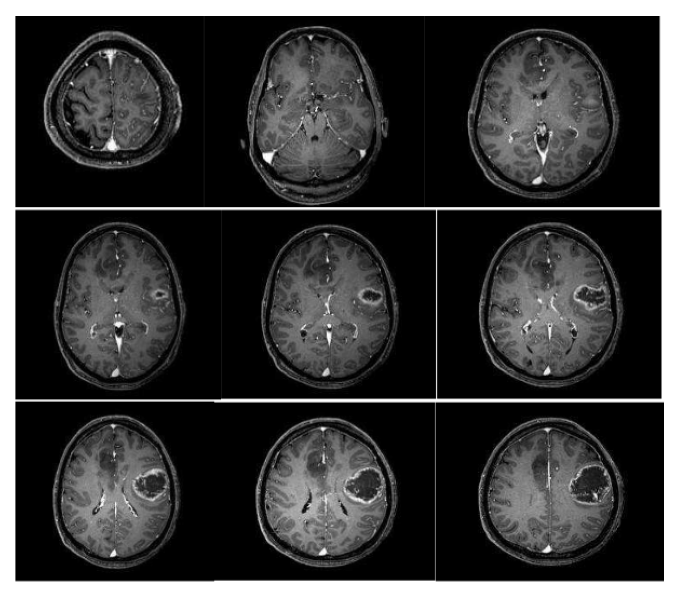
Figure 1. Tumor images.
Mca 30 00119 g001
Figure 2. Impact of chemotherapy on tumor and immune cells for the logistic growth model.
Mca 30 00119 g002
Figure 3. Impact of chemotherapy on tumor and immune cells for the exponential growth model.
Mca 30 00119 g003
Figure 4. Impact of chemotherapy on tumor and immune cells for the Gompertz growth model.
Mca 30 00119 g004
Figure 5. Effect of drug killing parameters b Ł , b , and b τ on tumor and immune cells.
Mca 30 00119 g005
Table 1. Differences between cancerous and non-cancerous tumors.
TraitBenignMalignant
Nuclear sizeSmallLarge
Ratio of nuclear size to cytoplasmic volumeLowHigh
Nuclear shapeRegularPleomorphic (irregular shape)
Mitotic indexLowHigh
Tissue organizationNormalDisorganized
DifferentiationWell differentiationPoorly differentiated
Tumor boundaryWell definedPoorly defined
Table 2. Numeric values of parameters.
ParameterDescriptionUnitValueReference
a 1 growth rate of tumor cellsday−1 4.31 × 10 1 [18]
a 2 tumor carrying capacitycell−1 5.14 × 10 1 [10]
a 3 tumor death by NK cellsday−1 3.5 × 10 6 [18]
a 4 growth rate of NK cellsday−1 5.14 × 10 1 [10]
a 5 carrying capacity of NK cellscell−1 1.0 × 10 7 [18]
a 6 NK cell death by tumorcell−1 day−1 1.0 × 10 7 [18]
β 1 tumor death by cytotoxic cellscell−1 day−1 1 × 10 4 Assumed
β 2 cytotoxic cell death by tumorcell−1 day−1 3.42 × 10 10 [10]
wnatural death of CTLsday−1 2 × 10 2 [18]
ractivation rate of CTLsday−1 1.6 × 10 7 Assumed
ρ natural death of NK cellsday−1 4.12 × 10 2 Assumed
b death rate of NK cells by drugday−1 6 × 10 1 [10]
b Ł death rate of CD8+ cells by drugday−1 0.0009 Assumed
b τ death rate of tumor cells by drugday−1 8 × 10 1 [10]
κ drug influxday−1 0.85 , 1.15 , 1.90 , 5.15 Assumed
C o drug decayday−1 0.95 , 1.25 , 2.10 , 5.25 Assumed
Table 3. Comparison of the logistic, exponential, and Gompertz models.
LogisticExponentialGompertz
Parameters: 16Parameters: 14Parameters: 16
State variables: 4State variables: 4State variables: 4
Identical behavior of tumor cells for κ = 0.85 Identical behavior of tumor cells for κ = 0.85 Identical behavior of tumor cells for κ = 0.85
Tumor and cytotoxic T cells decline rapidly for κ = 0.85 , 1.15 , and 1.90 while NK cells show variationTumor and cytotoxic T cells decline rapidly for κ = 0.85 , 1.15 , and 1.90 while NK cells show variationTumor and cytotoxic T cells decline rapidly for κ = 0.85 , 1.15 , and 1.90 while NK cells show variation
The decline of NK and CTL cells is rapid but better than exponential and Gompertz for κ = 5.15 Immune cells decrease more rapidly as compared to logistic for κ = 5.15 The decline of NK and CTL cells is more rapid than logistic but identical to exponential for κ = 5.15
Table 4. Comparison with existing works.
ReferenceState Variables/TherapyGrowth Model
[4]6, Chemotherapy and chemo-immunotherapyLogistic
[5]2, RadiotherapyLogistic
[6]3, Immunotherapy and chemotherapyLogistic
[10]4, ChemotherapyLogistic
[14]4, ChemotherapyLogistic
[15]4, VirotherapyLogistic
[16]4, Chemotherapy and immunotherapyLogistic
[18]6, Chemo-immunotherapyLogistic and Linear
[19]3, ImmunotherapyLogistic
[23]4, Chemotherapy, fractional derivative, and diffusion termLogistic
[24]4, Chemotherapy, radiotherapy, and immunotherapyExponential
[29]3, Interaction of immune cells and tumor cellsExponential
[30]6, Chemo-immunotherapyLogistic
[32]4, Fractional informed neural networkLogistic
[33]6, ChemotherapyLogistic
Current Paper4, ChemotherapyLogistic, Gompertz, and Exponential
Disclaimer/Publisher’s Note: The statements, opinions and data contained in all publications are solely those of the individual author(s) and contributor(s) and not of MDPI and/or the editor(s). MDPI and/or the editor(s) disclaim responsibility for any injury to people or property resulting from any ideas, methods, instructions or products referred to in the content.