Abstract
Kaniadakis deformed -mathematics is an area of mathematics that has found relevance in the analysis of complex systems. Specifically, the mathematical framework in the context of a first-order decay -differential equation is investigated, facilitating an in-depth examination of the -mathematical structure. This framework serves as a foundational platform, representing the simplest non-trivial setting for such inquiries which are demonstrated for the first time in the literature. Finally, additional avenues of study are discussed.
1. Introduction
In recent decades, the deformed statistics of Kaniadakis [1,2,3,4,5,6] have gained popularity as they have been applied to a wide array of disciplines such as cosmology [7,8,9,10], economics [11,12], and epidemiology [13,14], to cite but a few references. These so-called -statistics are predicated upon one parameter of a relativistically inspired generalization of the standard exponential as the -exponential (Figure 1(left)),
and the one-parameter relativistically inspired generalization of the usual logarithm as the -logarithm (Figure 1(right)),
where is a deformation parameter (sometimes also known as the entropic index), ranging in values between and 1.
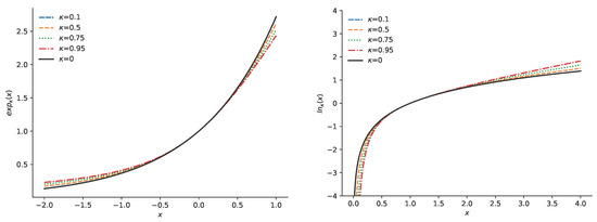
Figure 1.
Examples of -exponential (left) and -logarithm (right) for various values of the deformation parameter . Note that when , then -exponential and -logarithm approach the standard exponential and logarithm.
Kaniadakis -statistics are important because they provide a generalized statistical framework that extends the classical Boltzmann–Gibbs statistical mechanics to systems where standard assumptions—like extensivity, short-range interactions, or Markovian dynamics—may not hold. This is particularly relevant for complex systems with the following:
- Long-range interactions;
- Fractal or multifractal structure;
- Relativistic effects;
- Non-equilibrium steady states.
In these types of complex systems, power-law tails instead of exponential ones are generated. The -exponential is able to naturally generate distributions such as these.
There are some issues with -statistics. Outside the specific context of relativistic statistical mechanics (which is the inspiration for -statistics), by which the -statistics framework was originally motivated, the physical meaning of the deformation parameter is often ambiguous. Unlike physical constants (like Planck’s constant or the speed of light), is typically introduced as a phenomenological parameter without a direct derivation from first principles in many applications.
As a result, many times, it is unclear how to interpret the -parameter. In these cases, the -parameter effectively becomes a free parameter that can be adjusted in order to fit data and explore different regimes of the distribution functions.
In such cases, functions more like a modeling knob than a physically grounded variable, which may limit the predictive power and falsifiability of models that use it.
As the deformation parameter approaches zero,
the -exponential and -logarithm approach the standard exponential and natural logarithm, respectively. The -exponential and -logarithm are inverses of one another,
Probability distributions with power-law tails are ubiquitous in the natural sciences, and this makes these functions interesting. As mentioned above, some examples of phenomena described by the -statistics are the cosmic ray spectrum [15], which extends over 13 decades in energy and 33 decades in particle flux, with low-energy particles obeying an exponential distribution, whilst at high energies, the spectrum exhibits a power-law tail. The impact of loads on buildings and structures is effectively modeled [16] using -statistics. In this framework, the -exponential distribution accurately represents normal design loading conditions, while the tails of the distribution follow a power law pattern, reflecting the effects of loads that exceed the design values.
The natural question to ask within the framework of these deformed statistics is what is the physical meaning of the -deformation parameter? This deformation parameter has been introduced to describe deviations from the standard exponential behavior, especially in various probability distributions such as the exponential, Gaussian, weibull, and pareto distributions. In complicated physical systems, these deformations tend to be related to processes composed of short-range interactions, various correlations, or long-term memory effects. These deformations furthermore describe systems that are not in equilibrium or have a complex hierarchical nature, such as fractal systems.
At this point, it is appropriate to draw attention to another well-known generalized deformed statistical framework, Tsallis statistics [17,18,19], and to briefly compare it with the Kaniadakis formulation. Since the Tsallis framework is more widely recognized in the literature, such a comparison serves to place the present discussion within the broader context of deformed statistical mechanics.
Kaniadakis and Tsallis statistics represent two prominent generalizations of the Boltzmann–Gibbs framework developed to describe complex systems that deviate from classical extensivity. Both theories introduce a single deformation parameter that modifies the standard exponential and logarithmic functions, giving rise to power-law distributions capable of modeling long-range correlations, fractal structures, and non-equilibrium steady states. In Tsallis statistics, the deformation parameter q emerges from nonadditive entropy , leading to q-exponentials that break the additivity of entropy and capture nonextensive thermodynamics. In contrast, Kaniadakis statistics introduce a deformation parameter derived from relativistic symmetries, producing -exponentials that preserve additivity but deform the underlying algebra in a way that is consistent with special relativity. Consequently, while both frameworks yield heavy-tailed distributions and are reduced to the Boltzmann–Gibbs limit of or , Tsallis statistics are rooted in nonextensive entropy composition, whereas Kaniadakis statistics maintain entropy extensivity within a deformed relativistic mathematical structure.
The motivation of this work arises from the growing significance of Kaniadakis -statistics as a relativistically inspired generalization of Boltzmann–Gibbs statistical mechanics. This framework extends the classical exponential and logarithmic functions through the deformation parameter , allowing for the description of complex systems characterized by long-range interactions, fractal structures, relativistic effects, and non-equilibrium steady states. Although now applied in diverse areas, as already mentioned, such as cosmology, plasma physics, and information theory, the -formalism is often presented with few detailed explanations of its differential foundations accessible to new researchers. This study presents a systematic and accessible analytical exposition of the simplest nontrivial -deformed dynamical system, namely the first-order -deformed decay differential equation, with the goal of forming a pedagogical connection between classical and deformed calculus frameworks.
The principal result of this work is the introduction and validation of -exponential as a solution to the -deformed decay differential equation. This relationship demonstrates how deformation modifies the familiar exponential decay law within the -statistical framework. The equivalence of this solution is confirmed through a variety of independent analytical and numerical techniques, including direct substitution, separation of variables, the integrating-factor and WKBJ methods, Laplace and Lagrange–Charpit approaches, Picard’s iterative method, power-series expansion, and several numerical algorithms (Euler, Adams, and Runge–Kutta). The agreement among these approaches establishes both the internal consistency of -differential calculus and also highlights the unity of the deformed and classical frameworks, where each technique illuminates a different aspect of the same underlying structure.
The organization of this paper is as follows. Section 2 provides the motivation and mathematical preliminaries of -calculus, including the -exponential, -logarithm, and their algebraic properties. Section 3 introduces the -deformed decay equation and applies multiple analytic methods to obtain its solution. Section 4 extends the analysis to the Laplace and Lagrange–Charpit techniques, while Section 5 presents iterative and series approaches. Section 6 compares several numerical methods with the analytic solution to assess convergence and accuracy. Finally, Section 7 summarizes the findings and outlines future applications to more complex -deformed equations, such as -logistic, -advection, -wave, -diffusion, and -Fokker–Planck models.
2. Preliminaries
Much of the material presented in this section has been adapted and consolidated from established references on -mathematics and related works by Kaniadakis and others [1,2,4,5,6]. It is reproduced here for completeness and to ensure that the exposition is self-contained and accessible to readers new to the -formalism.
Arguably, the most interesting aspect of the -exponential is that it exhibits an exponential behavior at small values of x,
whilst exhibiting a power law behavior at asymptotic values of x (that is, the tail exhibits a power law structure),
(see Figure 2).
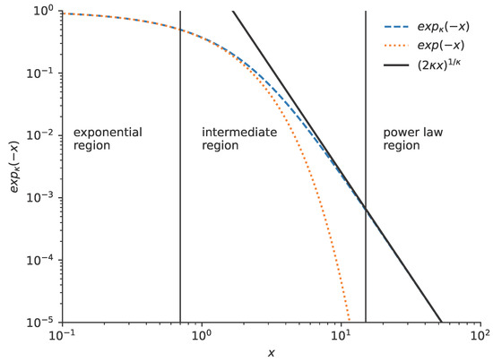
Figure 2.
The figure above shows the various regions of the -exponential (blue dashed curve), the exponential (red dashed curve), and a power-law (solid black curve). The parameter has the value of 0.75 in the above plots.
The Kaniadakis -exponential is defined by Equation (1). Expanding the square root using the first-order Taylor series for small x,
Applying the logarithm property reveals that,
Using the Taylor series expansion of for small u,
thus, the logarithm can be rewritten as
Since the last two terms cancel, this results in
Thus,
The large x approximation of the -exponential follows by taking Equation (1), and for large x, the square root term can be approximated using the expansion,
Thus, the term inside the power simplifies to
Raising both sides to the power of ,
resulting in,
Similarly, the -logarithm is similar to the usual standard logarithm as small values of x,
as it also exhibits a power law tails for the asymptotic values of x,
The low x regime result can be seen by taking the Kaniadakis -logarithm, Equation (2), and expanding for small ,
Substituting these results into the definition of the ,
The numerator can be simplified as
The Kaniadakis -logarithm for the small x approximation as regime can be approximated as
Since for leads to , resulting in
rewriting in terms of absolute value,
The approximation for Large x as ( ) can be written as
Since for large x, the dominant term in the logarithm is
Rewriting in absolute-value form,
There are two identities that are useful when working with -mathematics,
and
The algebraic structure of the -algebra for with , whose -sum composition law is defined via
forms an abelian group. The group properties are given below:
- Associativity: ,
- Identity Element: ,
- Inverse Element: , and
- Commutativity: .
The algebraic structure for the and previously described has a -product composition law defined via
and this also forms an abelian group. The group properties are given below:
- Associativity: ,
- Identity Element: ,
- Inverse Element: , and
- Commutativity: .
Often it is useful to introduce the definition of the -number via
and its dual is given as
It is easy to show that the -differential is given as
and the -integral corresponds to,
The -exponential (see Figure 1) is defined by Equation (1) and written in terms of the hyperbolic sine function,
where the Taylor series expansion of the -exponential is determined to be
with the -logarithm (see Figure 1) defined by Equation (2), and writing in terms of the hyperbolic sine function,
where the Taylor series expansion of the -logarithm is determined to be
where the deformation parameter exists on the interval , and as , Equations (1) and (2) reduce to the usual logarithm and exponential functions. Equations (1) and (2) are inverses of each other, and thus the following property holds:
One of the most ubiquitous equations in physics is the linear first-order homogeneous decay differential equation [20],
where in this work, the rate function is taken to be constant and the initial condition is . In this particular instance, the rate of decrease is a function, , that is proportional to the value of itself, which leads to the well-known standard decaying exponential function,
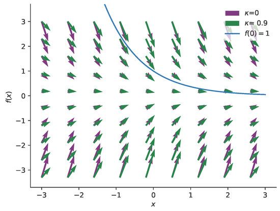
This equation describes radioactive half-lives, simple population decay, the discharge of a capacitor, and the rate law for certain first-order molecular reactions. In this work, the homogeneous first-order -differential equation (see the slope field in Figure 3),
will be studied, where again the rate function is taken to be a constant and the initial condition . The solution to this equation is analogous to the solution to Equation (45),
3. Techniques
In order to gain a deeper understanding of the -deformed framework, the deformed differential equation described in Equation (46) is solved by a variety of elementary methods to demonstrate the mathematical structure of the differential equation as well as the solution.
- Validation and verification: Validating and verifying solutions in the context of differential equations are important steps in the process of solving and understanding these equations and their solutions. These two steps ensure that the obtained solutions are accurate and consistent with the original differential equation and any initial or boundary conditions.
- Understanding: The -deformed statistics are not as well known as standard statistics or other deformed statistics (such as Tsallis statistics). This is an opportunity to investigate these statistics, in particular the deformed exponential and the deformed decay equation, from which a solution can be obtained within a familiar framework. By exploring a variety of methods for solving the same differential equation, valuable experience and insights that contribute to a deeper understanding of both the equation itself and its solutions can be acquired.
- Rigor: Solving a problem through various methods introduces rigor by subjecting the solution to different analytical approaches, verification steps, and perspectives. This multiplicity of approaches helps ensure the robustness and reliability of the solution. It allows for cross-validation and comparison.
- Computational efficiency and Applicability: This presents an opportunity to examine this deformed differential equation and corresponding solution and to determine which methods are better for handling the additional complexities introduced by the deformation aspects of both the equation and solutions.
3.1. Direct Substitution
The method of Direct Substitution is a technique used to solve certain types of ordinary differential equations. This method involves substituting a proposed solution into the differential equation to check if it satisfies the differential equation. If the substituted solution works, it is the solution to the differential equation. This method is advantageous when wanting to confirm a guessed and given solution. Assuming the solution has the form of Equation (1) and taking the derivative yields,
and rearranging leads to Equation (46). This method provides an intuitive way to understand the relationship between the differential equation and the -exponential.
3.2. Separation of Variables I
The method of Separation of Variables is one of the most straightforward techniques to determine the solution to a differential equation. This method requires that the differential equation be written in the form
which can then be manipulated into the form
where direct integration can be applied in this situation.
3.3. Separation of Variables II
Another more interesting application of the method of Separation of Variables that was described in Section 3.2 can be applied to the -decay equation utilizing the -numbers described by Equation (39).
3.4. Integrating Factor
The technique of the Integrating Factor [21,22] is a special implementation of the Separation of Variables technique with the derivative product rule. It should be noted that the integrating factor can be identified as Green’s function [23] when dealing with a non-homogenous first-order differential equation. This method requires the first-order differential equation of interest to be of the form
where this looks somewhat like the derivative of . In order to be a separable equation, the following is required:
which leads to the separable equation,
where the solution is
and the integration factor, , is
3.5. WKBJ
The Wentzel–Kramers–Brillouin-Jeffreys (WKBJ) method [24,25], though relatively specialized, can be applied to Equation (44) in order to determine the solution. It is assumed that the solution will be of the form
where A is a constant and satisfies the differential equation,
where
which leads to,
Substituting the result for the exponential’s exponent, Equation (53), into the test function, Equation (52), leads to
where in order to satisfy the initial condition that results in the solution, Equation (47).
4. Laplace and Lagrange–Charpit Techniques
4.1. Laplace Transform
Laplace transform is a technique to reduce a differential equation into an algebraic equation. The Laplace transform of the function is denoted by and is defined by,
It should be noted that, in order to ensure this integral’s convergence, while . This is in conflict with the Laplace transform that requires a non-negative domain. In order to ensure the applicability of the Laplace transform, will be restricted to the half-domain, .
Rewriting Equation (44) using the -numbers defined by Equations (37) and (38),
which can be re-written as
where the notation of the expression has been simplified using the ′-notation to describe the derivative with respect to . Applying the Laplace transform, ,
which leads to
where the Laplace transform of a sum is the sum of Laplace transforms and the Laplace transform of zero is simply zero. Applying the Laplace transform for a derivative,
to Equation (54) leads to
using the inverse Laplace transform to Equation (55) leads to
where the inverse Laplace transform is known to be
which leads to the result
and applying the initial condition that leads to the result of Equation (47).
4.2. Lagrange–Charpit Method
The Lagrange–Charpit method [26], also known as the Method of Characteristics, is a technique for solving hyperbolic differential equations.
Consider the partial differential equation of the form,
The solution surface is defined by characteristic curves that satisfy the system,
If , the system defines characteristic curves in the space. However, if , the equation is not defined, indicating that the solution depends only on x. In such cases, the system reduces to the following,
which describes single-variable characteristic curves. This method is now applied to the -deformed decay equation, Equation (46), given by
Setting and defining , the equation is rewritten as
The Lagrange–Charpit characteristic equations are then given by
Computing the necessary derivatives,
Substituting these into the characteristic equations,
Solving for , the first equation,
is separable. Integrating both sides,
Using the standard integral,
Solving for x,
Solving for from the second equation,
and integrating it,
Using , the substitution yields the following,
Defining the integration constants as a single constant, , results in
Exponentiating both sides,
Since
this simplifies to
Applying the initial condition ,
Since , it follows that ; thus,
Recognizing that,
leading to the solution, Equation (47).
5. Iterative and Series Approaches
5.1. Picard’s Iterative Method
Picard’s method [27,28], sometimes known as the Method of Successive Approximations, is a technique where one transforms a differential equation of the form
The method constructs an iterative sequence according to the integral equation,
The process begins with an initial approximation , typically chosen as the given initial condition, and refines the solution through successive iterations. If the iterations converge, the sequence approaches the exact solution of the differential equation.
Taking the -deformed decay equation, Equation (46), and rearranging it into standard form
establishes the recursive formulation,
The first iteration, (), is obtained by setting , leading to
Since the integral is evaluated to be
it follows that,
The second iteration, (), substituting into the iteration formula, is
Expanding as a Taylor series,
allows for the approximation
Thus, the integral simplifies to,
Approximating , the integration yields
Simplifying this,
The next iteration, (), is
Following the same approximation procedure, the integration leads to
The Taylor series expansion of the -exponential is given by
A comparison between the computed approximations and the exact expansion confirms that Picard’s method successfully reproduces the first three terms of for .
The series solution for various highest orders is shown in Figure 4 along with the associated errors.
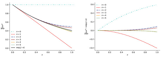
Figure 4.
The figure on the left is a comparison between the series solution (of various highest orders) from Picard’s method (see Equation (94)), the Power Series Method (see Equation (98)) and the exact solution, . The figure on the right is the difference between the power series truncated at order n and the -exponential.
5.2. Power Series Method
The Power Series Method seeks to determine a series solution by utilizing a trial power series solution [29]. The trial solution, along with its derivative, is taken to be
Substituting the ansatz into Equation (49) results in
and applying Taylor series to expand the square root,
Equating coefficients of various powers of x leads to the following relationships:
and
Using the initial condition that allows us to solve for , which then allows for the subsequent determination of the other coefficients, yielding
and
Substituting these coefficients back into Equation (96) results in
which results in the Taylor series described by the -decaying exponential, again yielding the solution, Equation (47).
6. Numerical Methods
Analytically solving the majority of ordinary differential equations, especially in physical contexts, is often challenging or even impossible. However, numerous numerical methods are available for effectively addressing and solving these types of equations. The focus of this work will be on the three commonly applied methods of Euler, Adam, and Runge–Kutta.
6.1. Euler’s Method
Euler’s method serves as an approximation to the solution with initial conditions. While this method may not be the most accurate approximation for practical situations, it stands out as the most straightforward approach for numerical calculation purposes. Rewriting Equation (46),
where depends on both the independent variable x and the dependent variable and where the initial condition is , the idea for using Euler’s method is to approximate the tangent line of the curve at equally spaced intervals . The general equation of the tangent line is
By choosing points , a better approximation can be obtained as gets closer to . As a result, the approximation can further be refined as the distance between and gets smaller, which in turn allows for an approximation of . This refinement feeds back into even subsequent approximations for .
This is written as
where is the step size. By iterating through, the approximate numerical solution to the differential equation can be determined.
Euler’s method was applied to the -deformed decay differential equation, Equation (46), and the results and numerical errors, along with the analytic solution and comparison to other numerical methods, can be seen in Figure 5.
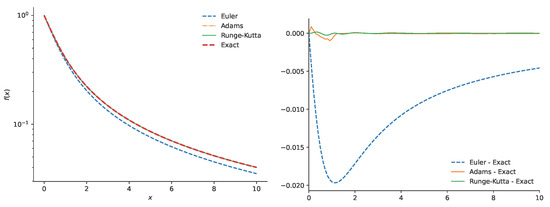
Figure 5.
The figure on the left is a comparison between the various numerical methods (Euler, Adam, and Runge–Kutta) and the exact solution to Equation (44). The figure on the right is the difference between various numerical methods and the exact solution.
6.2. Adam’s Method
Adam’s method is a multi-step algorithm to find approximate solutions to
This method is attractive due to the fact that it is typically more accurate than Euler’s method, and there is a gain in efficiency requiring only the use of the previous two approximations. Using the approximation,
where is the step size.
6.3. Runge–Kutta Method
The Runge–Kutta method is the most widely used technique for the numerical solution of general first-order differential equations and stands out as the most accurate among the numerical methods discussed here. It is employed to generate a highly accurate higher-order numerical method without the need for calculating higher-order derivatives. The general form of the Runge–Kutta method is
where the fourth-order Runge–Kutta method is given as
where is the step size and the slope estimates of the weighted average are given as
and
7. Conclusions
The objective of this study was to apply elementary methods to solving the deformed -exponential decay differential equation in order to gain experience with deformed statistics, in particular the -deformed exponential at the undergraduate level. The application of these techniques to Equation (46) has not been found in the literature, except for the method of Separation of Variables which was applied to
with the initial condition that and where is a constant. This resulted in a solution,
Any of the elementary methods that were applied in this work could be applied to Equation (99).
Now that there is experience with the deformed exponential and the deformed decay differential equation, this knowledge can be applied to studying similar differential equations such as the following:
- the -logistic differential equation would be an example of the next level of complexity,The solution to the standard logistics differential equation as well as the expected deformed solutions,where the solutions along with numerical errors have been plotted in Figure 6.
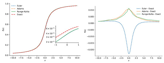 Figure 6. The figure on the left is a comparison between the various numerical methods (Euler, Adam, and Runge–Kutta) and the exact solution to the -deformed logistic equation, Equation (100). The figure on the right is the difference between various numerical methods and the exact solution.
 - analogous differential equations that are important in transport phenomena physics: differential equations such as,
- (a)
- The -advection equation,where u is the constant velocity associated with the advection,
- (b)
- -wave equation,where v is the speed of the wave,
- (c)
- -diffusion equation (and other Schrodinger-like equations),where D is the diffusion constant (the -diffusion equation has been examined for the first time by [30,31]), and
- (d)
- -Fokker–Planck equation,where D is a diffusion constant and is a drift constant. The -Fokker–Planck equation has been preliminary studied by [32,33].
- Fractional differential equations: these differential equations of non-integer order are used to more accurately model complex phenomena. They utilize fractional derivative operators such as the Caputo derivative. Preliminary work in this emerging field can be found in [34].
- Expansion of techniques: methods such as Laplace and Fourier transforms [35,36] have only begun to be investigated and there is still much work to do. In this work, the Laplace transform was performed using the -numbers. In the works cited, the authors investigated the -Laplace transform and the -Fourier transform.
Author Contributions
Conceptualization, J.A.S.; methodology, R.B., I.J. and J.A.S.; software, R.B. and I.J.; validation, R.B., I.J. and J.A.S.; formal analysis, R.B., I.J. and J.A.S.; investigation, R.B., I.J. and J.A.S.; writing—original draft preparation, R.B. and I.J.; writing—review and editing, R.B., I.J. and J.A.S.; supervision, J.A.S.; project administration, J.A.S. All authors have read and agreed to the published version of the manuscript.
Funding
This research received no external funding.
Data Availability Statement
No new data were created or analyzed in this study. Data sharing is not applicable to this article.
Acknowledgments
J. A. Secrest would like to thank J. M. Conroy at the State University of New York at Fredonia for many enlightening and stimulating conversations about the -formalism. R. Bolle and I. Jarra gratefully acknowledge the financial support of the College of Science and Mathematics at Georgia Southern University.
Conflicts of Interest
The authors declare no conflicts of interest.
References
- Kaniadakis, G. Non-linear kinetics underlying generalized statistics. Phys. A Stat. Mech. Appl. 2001, 296, 405–425. [Google Scholar] [CrossRef]
- Kaniadakis, G. Statistical mechanics in the context of special relativity. Phys. Rev. E 2002, 66, 056125. [Google Scholar] [CrossRef]
- Kaniadakis, G.; Scarfone, A.M. A new one-parameter deformation of the exponential function. Phys. A Stat. Mech. Appl. 2002, 305, 69–75. [Google Scholar] [CrossRef]
- Kaniadakis, G. Statistical mechanics in the context of special relativity. II. Phys. Rev. E 2005, 72, 036108. [Google Scholar] [CrossRef] [PubMed]
- Guha, P. Balanced gain-loss dynamics of particle in cyclotron with friction, κ-defomed logarithmic Lagrangians and fractional damped systems. Eur. Phys. Plus 2022, 137, 64. [Google Scholar] [CrossRef]
- Guha, P. The κ-deformed entropic Lagrangians, Hamiltonian dynamics and their applications. Eur. Phys. J. Plus 2022, 137, 932. [Google Scholar] [CrossRef]
- Luciano, G.G. Gravity and Cosmology in Kaniadakis Statistics: Current Status and Future Challenges. Entropy 2022, 24, 1712. [Google Scholar] [CrossRef]
- Abreu, E.M.; Neto, J.A.; Mendes, A.C.; Bonilla, A.; de Paula, R.M. Cosmological considerations in Kaniadakis statistics. Europhys. Lett. 2018, 124, 30003. [Google Scholar] [CrossRef]
- Lourek, I.; Tribeche, M. On the role of the κ-deformed Kaniadakis distribution in nonlinear plasma waves. Phys. A Stat. Mech. Appl. 2016, 441, 215–220. [Google Scholar] [CrossRef]
- Abreu, E.M.C.; Neto, J.A. Statistical approaches and the Bekenstein bound conjecture in Schwarzschild black holes. Phys. Lett. B 2022, 835, 137565. [Google Scholar] [CrossRef]
- Clementi, F. The Kaniadakis Distribution for the Analysis of Income and Wealth Data. Entropy 2023, 25, 1141. [Google Scholar] [CrossRef]
- Clementi, F.; Gallegati, M.; Kaniadakis, G. A New Model of Income Distribution: The κ-Generalized Distribution. J. Econ. 2012, 105, 63–91. [Google Scholar] [CrossRef]
- Kaniadakis, G.; Baldi, M.M.; Deisboeck, T.S.; Grisolia, G.; Hristopulos, D.T.; Scarfone, A.M.; Sparavigna, A.; Wada, T.; Lucia, U. The κ-statistics approach to epidemiology. Sci. Rep. 2020, 10, 19949. [Google Scholar] [CrossRef] [PubMed]
- Kaniadakis, G. Novel class of susceptible–infectious–recovered models involving power-law interactions. Phys. A Stat. Mech. Appl. 2024, 633, 129437. [Google Scholar] [CrossRef]
- Luciano, G.G. Kaniadakis entropy in extreme gravitational and cosmological environments: A review on the state-of-the-art and future prospects. Eur. Phys. J. B 2024, 97, 80. [Google Scholar] [CrossRef]
- Bushinskaya, A.; Timashev, S. Application of Kaniadakis κ-statistics to Load and Impact Distributions. In Proceedings of the 6th International Conference on Construction, Architecture and Technosphere Safety, Sochi, Russia, 10–16 September 2023; Springer: Cham, Switzerland, 2023. [Google Scholar]
- Tsallis, C. Possible generalization of Boltzmann–Gibbs statistics. J. Stat. Phys. 1988, 52, 479–487. [Google Scholar] [CrossRef]
- dos Santos, R.J.V. Generalization of Shannon’s theorem for Tsallis entropy. J. Math. Phys. 1997, 38, 4104–4107. [Google Scholar] [CrossRef]
- Lyra, M.L.; Tsallis, C. Nonextensivity and multifractality in low-dimensional dissipative systems. Phys. Rev. Lett. 1998, 80, 53–56. [Google Scholar] [CrossRef]
- Hobbie, R.K.; Roth, B.J. Exponential Growth and Decay. In Intermediate Physics for Medicine and Biology; Springer: New York, NY, USA, 2007. [Google Scholar]
- Krogstad, S. Generalized integrating factor methods for stiff PDEs. J. Comput. Phys. 2005, 203, 72–88. [Google Scholar] [CrossRef]
- Anco, S.C.; Bluman, G. Integrating factors and first integrals for ordinary differential equations. Eur. J. Appl. Math. 1998, 9, 245–259. [Google Scholar] [CrossRef]
- Melnikov, Y.A.; Borodin, V.N. Green’s Functions: Potential Fields on Surfaces; Springer: New York, NY, USA, 2017. [Google Scholar]
- Peters, J.M.H. Elementary but unusual methods of solving ordinary differential equations. Int. J. Math. Educ. Sci. Technol. 1982, 13, 295–297. [Google Scholar] [CrossRef]
- Keller, H.B.; Keller, J.B. Exponential-Like Solutions of Systems of Linear Ordinary Differential Equations. Rev. Soc. Ind. Appl. Math. 1962, 10, 246–259. [Google Scholar] [CrossRef]
- Delagado, M. The Lagrange–Charpit Method. Rev. Soc. Ind. Appl. Math. 1997, 39, 298–304. [Google Scholar]
- Tisdell, C.C. On Picard’s iteration method to solve differential equations and a pedagogical space for otherness. Int. J. Math. Educ. Sci. Technol. 2019, 50, 788–799. [Google Scholar] [CrossRef]
- Schelkunoff, S.A. Solution of linear and slightly nonlinear differential equations. Quart. Appl. Math. 1946, 3, 348–355. [Google Scholar] [CrossRef]
- Haarsa, P.; Pothat, S. The Frobenius Method on a Second-Order Homogeneous Linear ODEs. Adv. Stud. Theor. Phys. 2014, 3, 1145–1148. [Google Scholar] [CrossRef][Green Version]
- da Silva, M.V.; Martinez, A.S.; Gonçalves, A.C. Effective medium temperature for calculating the Doppler broadening function using Kaniadakis distribution. Ann. Nucl. Energy 2021, 161, 108500. [Google Scholar] [CrossRef]
- Wada, T.; Scarfone, A.M. On the Kaniadakis Distributions Applied in Statistical Physics and Natural Sciences. Entropy 2023, 25, 292. [Google Scholar] [CrossRef]
- Gomez, I.S.; da Costa, B.G.; dos Santos, M.A.F. Inhomogeneous Fokker–Planck equation from framework of Kaniadakis statistics. Commun. Nonlinear Sci. Numer. Simul. 2023, 119, 107131. [Google Scholar] [CrossRef]
- Hirica, I.E.; Pripoae, C.L.; Pripoae, G.T.; Preda, V. Lie Symmetries of the Nonlinear Fokker-Planck Equation Based on Weighted Kaniadakis Entropy. Mathematics 2022, 10, 2776. [Google Scholar] [CrossRef]
- Perovano, A.P.; Silva, F.S. Fractional operators with Kaniadakis logarithm kernels. Intermaths 2022, 3, 37–49. [Google Scholar] [CrossRef]
- Scarfone, A.M. κ-deformed Fourier transform. Phys. A Stat. Mech. Appl. 2017, 480, 63–78. [Google Scholar] [CrossRef]
- Kaniadakis, G. Theoretical Foundations and Mathematical Formalism of the Power-Law Tailed Statistical Distributions. Entropy 2013, 15, 3983–4010. [Google Scholar] [CrossRef]


Disclaimer/Publisher’s Note: The statements, opinions and data contained in all publications are solely those of the individual author(s) and contributor(s) and not of MDPI and/or the editor(s). MDPI and/or the editor(s) disclaim responsibility for any injury to people or property resulting from any ideas, methods, instructions or products referred to in the content. |
© 2025 by the authors. Licensee MDPI, Basel, Switzerland. This article is an open access article distributed under the terms and conditions of the Creative Commons Attribution (CC BY) license (https://creativecommons.org/licenses/by/4.0/).