Article

Regression Modeling for Cure Factors on Uterine Cancer Data Using the Reparametrized Defective Generalized Gompertz Distribution

by
Dionisio Silva-Neto
1,2,*,
Francisco Louzada-Neto
2 and
Vera Lucia Tomazella
1
1
Institute of Mathematics and Computer Sciences, University of São Paulo, São Carlos 13566-590, Brazil
2
Department of Statistics, Federal University of São Carlos, São Carlos 13565-905, Brazil
*
Author to whom correspondence should be addressed.
Math. Comput. Appl. 2025, 30(5), 93; https://doi.org/10.3390/mca30050093
Submission received: 14 July 2025 / Revised: 21 August 2025 / Accepted: 29 August 2025 / Published: 31 August 2025
(This article belongs to the Special Issue Statistical Inference in Linear Models, 2nd Edition)

Abstract

Recent advances in medical research have improved survival outcomes for patients with life-threatening diseases. As a result, the existence of long-term survivors from these illnesses is becoming common. However, conventional models in survival analysis assume that all individuals remain at risk of death after the follow-up, disregarding the presence of a cured subpopulation. An important methodological advancement in this context is the use of defective distributions. In the defective models, the survival function converges to a constant value p ( 0 , 1 ) as a function of the parameters. Among these models, the defective generalized Gompertz distribution (DGGD) has emerged as a flexible approach. In this work, we introduce a reparametrized version of the DGGD that incorporates the cure parameter and accommodates covariate effects to assess individual-level factors associated with long-term survival. A Bayesian model is presented, with parameter estimation via the Hamiltonian Monte Carlo algorithm. A simulation study demonstrates good asymptotic results of the estimation process under vague prior information. The proposed methodology is applied to a real-world dataset of patients with uterine cancer. Our results reveal statistically significant protective effects of surgical intervention, alongside elevated risk associated with age over 50 years, diagnosis at the metastatic stage, and treatment with chemotherapy.

1. Introduction

In recent years, medical studies have increasingly focused on improving the quality of life of patients with severe illnesses, such as cancer and other degenerative diseases. The study by [1] reports that the majority of patients living with HIV experience an improvement in their quality of life after initiating treatment. The authors also emphasize the relevance of psychiatric care and other complementary interventions as important contributors to enhancing and prolonging the quality of life of these patients. Ref. [2] presents a systematic review of randomized controlled trials evaluating supportive interventions aimed at improving the quality of life of prostate cancer patients. In this context, the term cancer survivor is defined as the broad experience across the cancer continuum, meaning living with, through, and beyond a cancer diagnosis. Ref. [3] reported that in 2005, around 170,000 individuals were diagnosed with primary lung cancer in the United States, with approximately 26,000 becoming long-term survivors each year, mainly due to improvements in treatment and surgery. Ref. [4] discusses studies that employ more potent, targeted therapies as an initial treatment strategy, particularly those capable of retaining effectiveness despite the development of resistance mutations or preventing such mutations from emerging. They found that such therapies can extend patient survival more effectively than delaying their use until resistance arises. The authors present a practical example of this in patients with ovarian cancer, where those who achieve a partial or complete response following platinum-based chemotherapy can experience an even more profound response with two years of maintenance therapy using olaparib. Clinical outcomes showed a 60% remission rate three years after initiating their inhibitor treatment, indicating an increase in the proportion of patients who are potentially cured.
In these contexts, although the traditional survival analysis approach remains essential, it often leads to several interpretative biases. This occurs because the vast majority of survival models assume that all individuals remain at risk of experiencing the event of interest, even after a long follow-up period. Therefore, it is crucial to account for the presence of a subgroup of patients who may become cured or immune to the event of interest, which could be, for example, death or disease recurrence. A conventional approach for modeling this phenomenon is the use of standard mixture cure models, originally proposed by [5] and further cited by [6]. These models define the population survival function as
S p ( t ) = ( 1 p ) + p S ( t ) ,
where p ( 0 , 1 ) represents the proportion of individuals who are not susceptible to the event of interest (i.e., cured or immune), and S ( t ) denotes the parametric survival function, which can be specified using distributions such as the Weibull, log-normal, log-logistic, among others. A characteristic feature of S p ( t ) is its improper behavior, as it converges to ( 1 p ) rather than zero as t . The extensions of this framework have introduced regression structures to model how covariates influence the probability of cure [7,8]. Despite its wide application, the standard mixture cure model requires the inclusion of an additional parameter (p) solely to capture the cure fraction, which may increase the complexity and burden of the inferential estimation process.
Ref. [9] introduced the concept of defective distributions as an alternative approach to model cure fractions in mixed populations. This class of distributions naturally exhibits an improper cumulative distribution function (CDF), meaning that F ( t ) does not integrate to one. This behavior arises from expanding the parameter space of one of the model’s parameters. Consequently, due to the intrinsic relationship between the survival function and the CDF, where S ( t ) = 1 F ( t ) , the survival function becomes defective naturally. This methodology offers advantages over standard mixture models by capturing the cure fraction as a function of the estimated parameters, eliminating the need to introduce an explicit additional parameter. Thus, the survival function converges to a value p ( 0 , 1 ) as t , which reflects the proportion of cured individuals. This class also offers an integrated approach, as the statistical estimation proceeds in the conventional manner when there is no evidence of cure in the population.
The main differences between standard mixture models and defective distributions in the context of cure rate models are as follows: (i) standard mixture models are structured to fit parametric (or nonparametric) models in the presence of long-term survivors, whereas defective models are naturally formulated without requiring a special structure that increases the dimension of the parameter vector; (ii) in standard mixture models, the cure fraction is treated as an additional parameter in the inference process, while in defective models, the survival function itself is used to capture the cure fraction, expressed as a function of the estimated parameters; and (iii) defective models provide an integrated approach in which one parameter always acts as an indicator of the presence of a cured fraction. In the absence of a cure fraction, inference proceeds conventionally as in a model where all individuals are susceptible to the event of interest. This third point is particularly relevant in scenarios where the cure fraction is not evident from descriptive survival curves, allowing the inferential process to serve as additional evidence in identifying situations that may involve long-term survivors.
Among defective distributions, the Gompertz distribution stands out in the literature for its natural defective behavior in scenarios involving cure fractions. Several studies have leveraged this property to propose parsimonious modeling approaches. In the work of [10], the defective Gompertz distribution was extended to the Marshall–Olkin family, where it was shown that the distribution remains defective, and an application to leukemia and colon cancer data presented a more appropriate fit in comparison with the baseline defective Gompertz model. Subsequently, ref. [11] extended the Gompertz distribution to the Kumaraswamy family, where the new defective form proved particularly relevant in the analysis of melanoma data, with the Kumaraswamy–Gompertz model outperforming its baseline counterpart according to frequentist criteria such as AIC, BIC, and CAIC. Furthermore, the extension proposed by [12] provided practical insights into breast cancer prognosis through a defective Beta–Gompertz model, offering interpretability regarding the role of clinical covariates in individual survival probabilities.
In this project, we adopt the generalized Gompertz distribution, proposed by [13], as a flexible modeling tool for continuous, non-negative random variables. We prefer to use this generalization of the defective Gompertz distribution because several studies in the literature have shown gains in statistical modeling for different probability distributions when incorporated into the Lehmann family [14,15,16]. In particular, the work of [17] highlights the defective generalized Gompertz distribution in a quantile regression framework, underscoring its potential in broader inferential settings. Our aim in this work is to provide an interpretable framework for identifying factors that may influence the probability of cure among long-term survivors. Specifically, we propose a framework over a defective survival model that allows clinical specialists to evaluate how clinical and treatment-related factors may either enhance or impair the quality of life of patients who show evidence of immunity to the disease.
The rest of this paper is organized as follows: in Section 2, we present the proposed methodology, discussing the construction of the defective regression model and the inferential process; in Section 3, we present a simulation study, describe the motivating dataset, and apply our proposed model, followed by a diagnostic evaluation; finally, in Section 5, we present the conclusions and discuss directions for future research.

2. Materials and Methods

2.1. The Defective Gompertz Distribution

In the conventional formulation, the Gompertz distribution is defined by two strictly positive parameters: α > 0 (the shape parameter) and μ > 0 (the scale parameter). The probability density function of the Gompertz distribution for a non-negative random variable and its corresponding survival function are, respectively,
f ( t ; α , μ ) = μ e α t μ α e α t 1 ,
S ( t ; α , μ ) = 1 0 f ( t ; α , μ ) d t = e μ α e α t 1 .
When the parametric space of α changes from ( 0 , ) to ( , 0 ) , the distribution becomes improper (it does not integrate 1), which is connected to the idea of a cure fraction in the data ( p 0 ), which can be easily computed as
p 0 = lim t S ( t ; α , μ ) = lim t e μ α e α t 1 = e μ α ( 0 , 1 ) .
The above expression implies that, once the values of α and μ are estimated, it is possible to obtain the proportion of the cure fraction in the data. This is a substantial advantage of this distribution compared to the traditional mixture cure model because the proportion of cure is intrinsically obtained from the survival function. This reduction of the components in the parametric vector leads to several benefits, such as improved estimation precision and simpler computations. Additionally, the model can be specified in an integrated way, where α R ; this means the cure fraction can be detected naturally depending on the value of the shape parameter.

2.2. The Defective Generalized Gompertz Distribution

To introduce greater flexibility to the defective Gompertz distribution, we work with its inclusion within the family of flexible distributions defined by [18], given by the cumulative distribution function:
G ( z ; θ , ψ ) = P ( Z z ) = F ( z ; θ ) ψ ,
where F ( z ; θ ) denotes the CDF of a random variable Z, indexed by the parameter vector θ . The parameter ψ > 0 introduces additional flexibility to the baseline distribution by modifying its shape. When ψ = 1 , the baseline model is recovered as a particular case.
We can easily derive the probability density and survival functions in Lehmann’s family, respectively.
g ( z ; θ , ψ ) = ψ f ( z ; θ ) F ( z ; θ ) ψ 1 ,
S G ( z ; θ , ψ ) = 1 F ( z ; θ ) ψ .
Based on Equations (5) and (6), applied to the probability density and survival functions of the Gompertz distribution, given in Equations (1) and (2), respectively, we obtain the following expressions for the probability density function and the survival function of the generalized Gompertz distribution:
f ( t ; α , μ , ψ ) = ψ μ e α t μ α e α t 1 1 e μ α e α t 1 ψ 1 ,
S ( t ; α , μ , ψ ) = 1 1 e μ α e α t 1 ψ ,
where α > 0 , μ > 0 , ψ > 0 , and t > 0 . This family of distributions was initially discussed by [13] and later extended into a broader class of distributions presented in [11].
A relevant question concerns whether the generalized Gompertz distribution can present a defective form and under which conditions this characteristic may occur. This distribution can be seen as a particular case of the defective distribution introduced by [11]. When one of the added parameters in the Kumaraswamy family takes the value 1, the model simplifies to the baseline structure discussed in this work. We opted not to adopt the most general version of the model, which incorporates two shape parameters, in order to achieve greater flexibility while preserving the principle of parsimony.
The generalized Gompertz distribution is defective when α < 0 (as is the case with the defective Gompertz distribution). The resulting model corresponds to the defective generalized Gompertz distribution (DGGD) as discussed by [17]. Given α < 0 , the proportion of the cure fraction can be easily computed as
p = lim t S ( t ; α , μ , ψ ) = lim t 1 1 e μ α e α t 1 ψ = 1 1 lim t e μ α e α t 1 ψ = 1 1 p 0 ψ ,
where p 0 = e μ / α is the computed cure fraction in the Gompertz defective distribution (Equation (3)).

2.3. Model with Covariates

In this section, we introduce the extension of the DGGD, which incorporates covariates and reparametrization. Our formulation aims to interpret the model in terms of the cure; we propose a reparametrized version in terms of the estimand p,
p = 1 [ 1 p 0 ] ψ = 1 1 e μ α ψ .
We propose substituting the scale parameter to maintain the identification of the cure fraction in terms of α and the flexibility in terms of ψ ,
p = 1 1 e μ α ψ μ = α ln 1 [ 1 p ] 1 ψ .
The new versions for the probability density and survival functions of the DGGD, in terms of α , ψ and p, are given as follows. To simplify the notation, consider η ( p ; ψ ) = ln 1 [ 1 p ] 1 ψ .
f ( t ; α , p , ψ ) = ψ α η ( p ; ψ ) e α t η ( p ; ψ ) e α t 1 1 e η ( p ; ψ ) e α t 1 ψ 1 ,
S ( t ; α , p , ψ ) = 1 1 e η ( p ; ψ ) e α t 1 ψ .
We include the covariate effects ( x i , i = 1 , 2 , , n ), where x i is the covariate information for the i-th observation, in the analysis of the cure parameter p to understand how clinical characteristics can influence the probability of being cured. Considering the parametric space of p, we apply the logistic link function
p ( x i ) = e x i β 1 + e x i β = 1 1 + e x i β ,
where x i = ( 1 , x i 1 , x i 2 , , x i q ) is a vector of observations from q independent variables for the i-th observation and β = ( β 0 , β 1 , , β q ) is the vector of regression coefficients.

2.4. Bayesian Inference

The Bayesian paradigm focuses on obtaining the joint posterior distribution π ( ϑ D ) , which results from combining prior knowledge (or ignorance) about the parameter vector ϑ , expressed through the prior distribution π ( ϑ ) , with the information provided by the data via the likelihood function L ( ϑ D ) . The posterior distribution is obtained by applying Bayes’ theorem,
π ( ϑ D ) = π ( ϑ ) × L ( ϑ D ) π ( D ) π ( ϑ ) × L ( ϑ D ) ,
where “∝” denotes the proportional information about ϑ .
Consider an independent sample of size n and an observed time of T i = min ( T i * , C i ) , where T i * is the true survival time and C i the censoring time, with δ i = I ( T i * C i ) being the failure indicator, let x i = ( 1 , x i 1 , x i 2 , , x i q ) be the observed variables affecting the individual cure rate for the i-th observation. Thus, the complete observed dataset is D = ( T i , δ i , x i ; i = 1 , , n ) . The vector of parameters is given by ϑ = ( α , ψ , β ) . The likelihood function for right-censored survival data can be expressed as
L ( ϑ D ) = i = 1 n f ( t i ; α , p i , ψ ) δ i × S ( t i ; α , p i , ψ ) ( 1 δ i ) = i = 1 n ψ α η ( p i ; ψ ) e α t η ( p i ; ψ ) e α t 1 1 e η ( p i ; ψ ) e α t 1 ψ 1 δ i × 1 1 e η ( p i ; ψ ) e α t 1 ψ ( 1 δ i ) .
Assuming independence among the components of the vector ϑ , the prior distribution is
π ( ϑ ) = π ( α ) π ( ψ ) k = 0 q π ( β k ) ,
where each component in the Bayesian regression defective generalized Gompertz model has the following prior specifications
β k Normal ( μ k , σ k 2 ) , k = 0 , 1 , 2 , , q .
α Normal ( m , s 2 ) ,
ψ gamma ( γ , ω ) ,
where ( μ k , σ k ) , k = 0 , 1 , 2 , , p ; m, s, γ , and ω are known hyperparameters. The choice of the priors for the coefficients associated with the covariates is based on the recommendation by [19]. The prior for the ψ parameter was chosen based on existing literature on Bayesian survival models for the Lehman family of distributions [20,21]. As for the α parameter, given the expansion of the parameter space, we required a prior over the real numbers, and the Gaussian distribution showed good results under the assumption of independence from the other parameters. Prior sensitivity studies were performed, and the configuration was deemed non-informative for the parameters of interest, as described in Section 1 in the simulation study.
However, the joint posterior density π ( ϑ D ) usually involves necessary integrals that are not easy to calculate, making it impossible to obtain a closed-form. To overcome this, the Markov Chain Monte Carlo (MCMC) method is used to obtain samples from π ( ϑ D ) , which enables inference on the parameter vector ϑ through summary statistics. Two famous algorithms to sample from the posterior distribution are Metropolis–Hastings [22,23] and Gibbs sampling [24]. However, a major challenge in these approaches lies in selecting an appropriate proposal density to ensure efficient sampling. One interesting alternative is the Hamiltonian Monte Carlo (HMC) [25,26], which is based on gradients of the objective distribution to propose samples adaptively, available in the rstan package [27].
The idea of HMC uses concepts of gradients and differential geometry on the posterior distribution. Ref. [28] provides a full description of the algorithm. We can describe ut briefly in the following steps:
(i)
The state space is augmented by momentum parameters; therefore, the parameter vector consists of the parameters of interest and the momentum parameters;
(ii)
We define the Hamiltonian function as the negative value of the logarithm of the joint distribution with all parameters;
(iii)
The momentum of all parameters is sampled from a multivariate Gaussian, typically from the current value of the parameters;
(iv)
The proposal distribution of parameters of interest is defined, conditioned on the gradients of the Hamiltonian function in the current value. Then, we consider the local geometry of the distribution.
The standard version of the HMC algorithm involves a large number of hyperparameters, which complicates the automation of the sampling process. These include the number of updates performed before the acceptance or rejection step (leapfrog steps), the step size (which follows the direction of the computed gradient), and the covariance matrix of the probability distribution for the momentum parameters. In the rstan package, an adaptive version of the leapfrog step is implemented to reduce the number of hyperparameters during tuning. The covariance matrix of momentum parameters is estimated during the warm-up period, as is the step-size, with the objective of improving the acceptance rate. The optimal number of updates is determined dynamically. The idea is to use enough updates to explore the parametric space efficiently. This occurs because the algorithm avoids retracing previously explored paths (U-turns) or halts the trajectory once a predefined maximum number of leapfrog steps is reached. The NUTS (No U-Turn Sampler) algorithm implemented in rstan employs multinomial sampling across the generated trajectory to select a sample [28,29]. If the leapfrog integration process fails, indicated by a significant deviation of the Hamiltonian value from its starting point, the trajectory is classified as divergent and is subsequently discarded.
Compared to conventional MCMC approaches, HMC demands greater computational resources per iteration, primarily due to the need for gradient evaluations. Nevertheless, this characteristic allows HMC to navigate complex posterior distributions with strong parameter correlations more efficiently than traditional MCMC methods. As a result, fewer iterations are generally required to obtain reliable parameter estimates and credible intervals, often leading to reduced overall computation time. Notably, ref. [30] showed that across various applications, HMC implemented in rstan consistently achieves a higher effective sample size per unit of computation than MCMC algorithms, such as those available in JAGS (Just Another Gibbs Sampler) software.
A key challenge with conventional MCMC algorithms is selecting proposal densities and, critically, determining the number of iterations needed to verify chain convergence. As cited by [31], this is a frequent point of criticism when Bayesian models rely on stochastic sampling for estimation. To address this challenge, we employed the Hamiltonian Monte Carlo (HMC) algorithm with the NUTS for our Bayesian model. By relying less on correlated samples during the burn-in period, due to NUTS’s ability to use automatic differentiation, we accelerated the execution of the Monte Carlo experiment in Section 3.1. We also believe that providing the code in the rstan software will facilitate peer review and replication, making it easier for others to identify the components of the log-likelihood and priors, along with their respective hyperparameters.
Computations were performed on a 12th-generation Intel Core i7 machine with 16 GB of unified RAM and a 250 GB SSD running on Linux Fedora 42. For explanatory purposes, in the simulation study presented in Section 3.1, we generated 5000 posterior samples, discarding the first 1000 as burn-in. The number of steps was set to 1 because the NUTS algorithm in HMC naturally produces low-correlation samples. Each iteration, using four CPU cores for two chains, took less than 2 min for the largest sample size considered (1000 observations) after finding good starting values in the first iteration.

2.5. Residual Analysis

In order to verify the error assumptions and the presence of outliers, we apply two types of residual analysis for our defective model for both inferences: a deviance component residual and a martingale-type residual. The martingale residuals are skewed; they have a maximum value of +1 and a minimum value of . In the parametric survival models, the martingale residuals can be expressed as
r M i = δ i + log ( S ( t i ; ϑ ) ) ,
where S ( t i ; ϑ ) is the survival function computed in sample data under the vector of parameters estimated ( ϑ ), and δ i is the indicator function for the occurrence of the event of interest.
The deviance component residual is a transformation of martingale residuals to lessen its skewness; this approach is the same for generalized linear models [32]. In particular, the deviance component residuals to a parametric regression model with explainable covariates can be expressed as
r D i = signal ( r M i ) { 2 [ r M i + δ i log ( δ i r M i ) ] } 1 / 2 ,
where r M i is the martingale residual.

3. Results

3.1. Simulation Study

We conducted a simulation study to evaluate consistency through frequentist properties of the Bayesian regression model using point and interval estimates. Let F ( t ) represent the cumulative function for the survival time associated with a specified event of interest, which can contain information about long-term survivors. Our goal is to generate the information of the observed survival time, the censoring indicator, and covariate information under a stochastic process. This procedure is clearly explained in Algorithm 1.
Algorithm 1 Dataset generation algorithm from the DGGD with covariates.
1:
Define the values of β = ( β 0 , β 1 , β 2 ) R 3 , α < 0 , and ψ > 0 ;
2:
for  i = 1 to n do
3:
    Define x i = (1, x i 1 , x i 2 ), where x i 1 Bernoulli ( 0.5 ) , x i 2 Normal ( 0 , 1 ) ;
4:
    Determine the individual cure rate
p i ( x i 1 , x i 2 ) = 1 1 + e x i β ;
5:
    Generate M i Bernoulli ( 1 p i ( x 1 , x 2 ) ) ;
6:
    if  M i = 0  then
7:
         Set t i * = ;
8:
    else
9:
        Take t i * as the root of F ( t ) = u , where u U ( 0 , 1 p i ( x i 1 , x i 2 ) ) and F ( t ) is the CDF of the defective generalized Gompertz distribution;
10:
    end if
11:
    Generate u i * U ( 0 , max ( t i * ) ) , considering only the finite values of t i * ;
12:
    Calculate t i = min ( t i * , u i * ) and δ i = 1 ( t i * u i * ) ;
13:
end for
14:
Output: The final dataset is D = { ( t i , δ i , x 1 i , x 2 i ) : i = 1 , 2 , , n } .
We evaluated four sample sizes ( n = 100 , 300 , 500 , 1000 ) over 1000 Monte Carlo replicates. In each iteration, we computed the posterior means ( ϑ ^ ) and the bias, given by B ( ϑ ^ ) = ( ϑ ^ ϑ ) , where ϑ is the vector of true values, and the function to check if each component of ϑ is covered by the 95% credible intervals. We conducted sensitivity studies of the prior distributions presented in Section 2. The model showed good estimation results with a considerable sample size ( n 300 ) when we considered the following configuration of vague priors: α Normal ( 1 , 10 2 ) , ψ Gamma ( 0.01 , 0.01 ) , and β k Normal ( 0 , 10 2 ) , k = 0 , 1 , 2 , , q . For better results in scenarios with a low number of sample observations, we recommend using more informative priors, especially for the parameters α and ψ .
For the simulation study, the vector of true values was chosen as ϑ = ( α = 0.15 , ψ = 0.70 , β 0 = 1.30 , β 1 = 1.30 , β 2 = 0.50 ) . These values were based on posterior means from the application in the Section 3.2, except for the effect β 2 , which was selected arbitrarily due to the lack of continuous covariates in the dataset. We chose to include this effect of a continuous variable in the Algorithm 1 to illustrate the capability of our regression model to handle such information. Convergence statistics ( R ^ ) based on two chains per iteration were close to 1 for all parameters across sample sizes. Figure 1 presents the values of the bias and the coverage probability across the sample sizes evaluated for the parameter vector ϑ .

3.2. Motivating Dataset

The dataset used in this study was provided by the Oncocenter Foundation of São Paulo (undação Oncocentro de São Paulo, FOSP), an institution linked to the São Paulo State Department of Health. The FOSP organizes clinical data from both public and private healthcare institutions across the state of São Paulo, which is systematically compiled within the Hospital Cancer Registry (HCR). The HCR includes information on cancer cases reported since the early 2000s, encompassing patients with or without a confirmed diagnosis, including individuals already undergoing treatment. In addition, the registry contains sociodemographic data and variables related to healthcare provision, providing a comprehensive overview of the oncology care profile. Using data from the HCR, we investigated cases of uterine cancer among women residing in the state of São Paulo between 2012 and 2020.
Uterine cancer can be broadly classified into two main subtypes: endometrial cancer and uterine sarcoma. Endometrial cancer originates in the inner lining of the uterus (the endometrium) and accounts for the vast majority of uterine cancer cases. According to [33], it is the fourth most frequently diagnosed cancer among women, following breast, colorectal, and lung cancer, and represents the seventh leading cause of cancer-related mortality in women. The highest prevalence is observed among postmenopausal, middle-aged, elderly, or obese women. The incidence of endometrial cancer is particularly high in Western countries and shows a strong association with rising obesity rates [33]. By the end of the 20th century, approximately 42,000 deaths were attributed to uterine cancer worldwide, with 27,500 occurring in developed countries and 14,400 in developing regions in 1990. For instance, in the United States, mortality rates from endometrial cancer doubled between 1988 and 1998, a trend likely driven by increased life expectancy and rising obesity rates, along with associated comorbidities [34,35]. In contrast, uterine sarcomas are rare tumors that develop in the myometrium (the muscular layer of the uterus) or in other supporting tissues. They represent approximately 1% of all female genital tract malignancies and 3–7% of uterine cancers [36]. Despite their rarity, uterine sarcomas exhibit highly aggressive behavior. Among these, carcinosarcomas are especially notable for their poor prognosis, with an estimated five-year overall survival of approximately 30%, increasing to about 50% for patients diagnosed at stage I, when the disease is confined to the uterus. The rarity and histopathological heterogeneity of uterine sarcomas have contributed to a lack of consensus regarding optimal treatment strategies and risk factors for poor outcomes [37].
In our study, we considered the failure time as the period between the date of the patient’s diagnosis of uterine cancer and the date of the last available information regarding their health status (cancer-free, living with uterine cancer, or death due to uterine cancer or other causes). The event of interest was defined based on death attributed to uterine cancer. The dataset contains 490 individuals, and the censoring proportion is approximately 0.4735. Figure 2 presents the nonparametric Kaplan–Meier estimator for the uterine cancer dataset, along with the 95% confidence interval. A plateau is observed after approximately 10 years of patient follow-up, suggesting the potential presence of cured individuals within the population.
To model the probability of cure, we included the following covariates: patient age categorized into two groups, distinguishing individuals over 50 years old (Age > 50); presence of distant recurrence, representing the occurrence of metastasis (Metastasis); whether the patient underwent surgery inside or outside the hospital (Surgery); whether the patient received chemotherapy inside or outside the hospital (Chemotherapy); and whether the patient received hormone therapy inside or outside the hospital (Hormone Therapy). We adopted vague prior distributions for the regression coefficients, as well as for the shape and power parameters of the DGGD, following the same specifications described in the simulation study in Section 3.1.
Table 1 shows that the DGGD exhibited a defective form, as evidenced by the negative estimated value of the parameter α , with statistical significance shown by the estimated 95% credibility interval.
Table 2 presents the values of the model comparison metrics DIC (deviance information criterion), PSIS-LOO (Pareto smoothed importance sampling for Leave-One-Out Cross validation), and −2*LPML (logarithm of pseudomarginal likelihood) for the regression cure models based on the Gompertz and generalized Gompertz distributions. All metrics choose the more appropriate model with the lowest value, and they are described in more detail in Appendix C.
PSIS-LOO is a powerful tool for model diagnosis that goes beyond simply estimating predictive accuracy. For a more detailed description, we strongly recommend [38]. The key diagnostic metric is the estimated Pareto shape parameter, k ^ , which assesses the reliability of the PSIS-LOO approximation for each data point. If k ^ is below 0.5, the approximation is highly stable. Values between 0.5 and 0.7 indicate a need for caution, as the approximation is less reliable. If k ^ exceeds 0.7 (and critically 1), it means that the approximation for that data point is problematic because the generalized central limit theorem of the method may not hold. In general, a high k ^ value suggests that the data point is highly influential and its removal significantly changes the posterior distribution, warranting further investigation as it may be an outlier or indicate problems with the specification of the model.
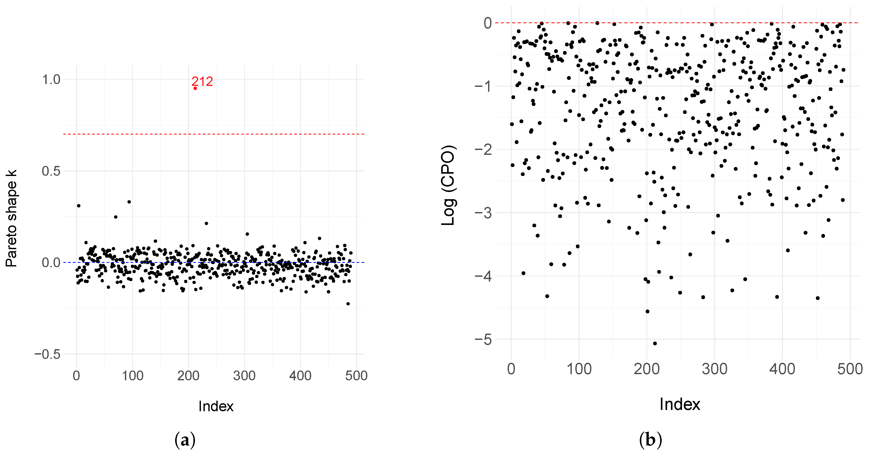
Figure 3 presents the PSIS-LOO individual values and the natural logarithm of the CPO values for identifying influential points in the estimation of the generalized Gompertz model.
Figure 4 presents the values of martingale residuals and deviance residuals, which are classical tools to identify outliers. The criteria to decide whether a parametric model contains many outliers, we pay attention to the values of deviance residuals outside the range of (−3, 3).

4. Discussion

Figure 1 shows the low bias for all parameters starting from a sample size of 300 observations. Specifically, the values are very close to zero, with differences only appearing in the third decimal place on average. Additionally, the coverage probability shows satisfactory values at the nominal level of 95% for all parameters when the sample size is equal to 300 individuals. Thus, the frequentist measures demonstrate that the defective regression model provides good asymptotic results under a vague priori scheme for sample sizes commonly found in datasets within the medical literature. In the dataset discussed in Section 3.2 about uterine colon cancer, the sample size is close to 500 observations, for which we have satisfactory results in Figure 1.
For the real-world application, based on the regression structure for the cure parameter and the estimated coefficients from the dataset, disregarding the effects of other covariates, the expected probability of cure for patients with uterine cancer, obtained from the estimated intercept applied to the logistic link function, is approximately 20%. Regarding other covariates, patients aged over 50 years exhibit, on average, a 14% reduction in the probability of cure, assuming no influence from additional treatments and factors. The positive estimated effect associated with surgery (1.8800), along with its corresponding 95% credible interval, indicates that surgical intervention has a beneficial and significant impact on increasing the probability of cure. A positive effect was also observed for hormone therapy (2.6224), although this result was not statistically significant. In contrast, the occurrence of metastasis, indicated by the presence of distant recurrence, and chemotherapy were identified as risk factors that reduce the probability of cure, given the negative estimated effects of these binary variables. The 95% credible interval of the chemotherapy highlights its statistical significance as very low in the long-term survival of female patients with uterine cancer.
When we evaluate the best proposal, based on the model selection metrics for Bayesian models, the results in Table 2 indicate that the values are substantially lower for the flexible defective version compared to the traditional form. Therefore, for the uterine cancer dataset, the most appropriate cure model is the one based on the generalized Gompertz distribution.
Figure 3 shows that the PSIS-LOO diagnostic plot for the DGGD indicated that most observations had reliable approximations, with Pareto k values below 0.7. However, one influential observation (212 data points) exceeded the threshold (k > 0.7), suggesting that the leave-one-out predictive distribution for this point is not well-approximated by importance sampling. This indicates this observation is a potential outlier with high leverage. On the other hand, the logarithmic values of the CPO for the defective generalized Gompertz model were relatively high, indicating higher CPO values and, consequently, good predictive performance. This suggests that the model provides an adequate fit in terms of prediction. In terms of outlier detection, Figure 4 shows that the martingale residuals are randomly scattered around zero, indicating that the defective regression model based on DGGD provides a reasonably good fit to the data. Only one outlier (284 data points) falls outside the range of (−3, 3) in the deviance residuals, which supports the adequacy of the model. Overall, the results provide evidence that the regression model appropriately captures the relationship underlying the cure fraction.
Appendix A presents the inferential summaries excluding observations 212 and 284, which were identified as influential and outlier points, respectively. Although the marginal standard deviations of some parameter estimates increased considerably, the statistical significance of most regression coefficients was preserved. When observation 212 was removed, the regression coefficient associated with hormonal treatment for uterine cancer remained statistically significant, while the presence of metastasis did not show a significant effect. Overall, the inferential summary without observation 212 was very similar to that obtained using the complete dataset.
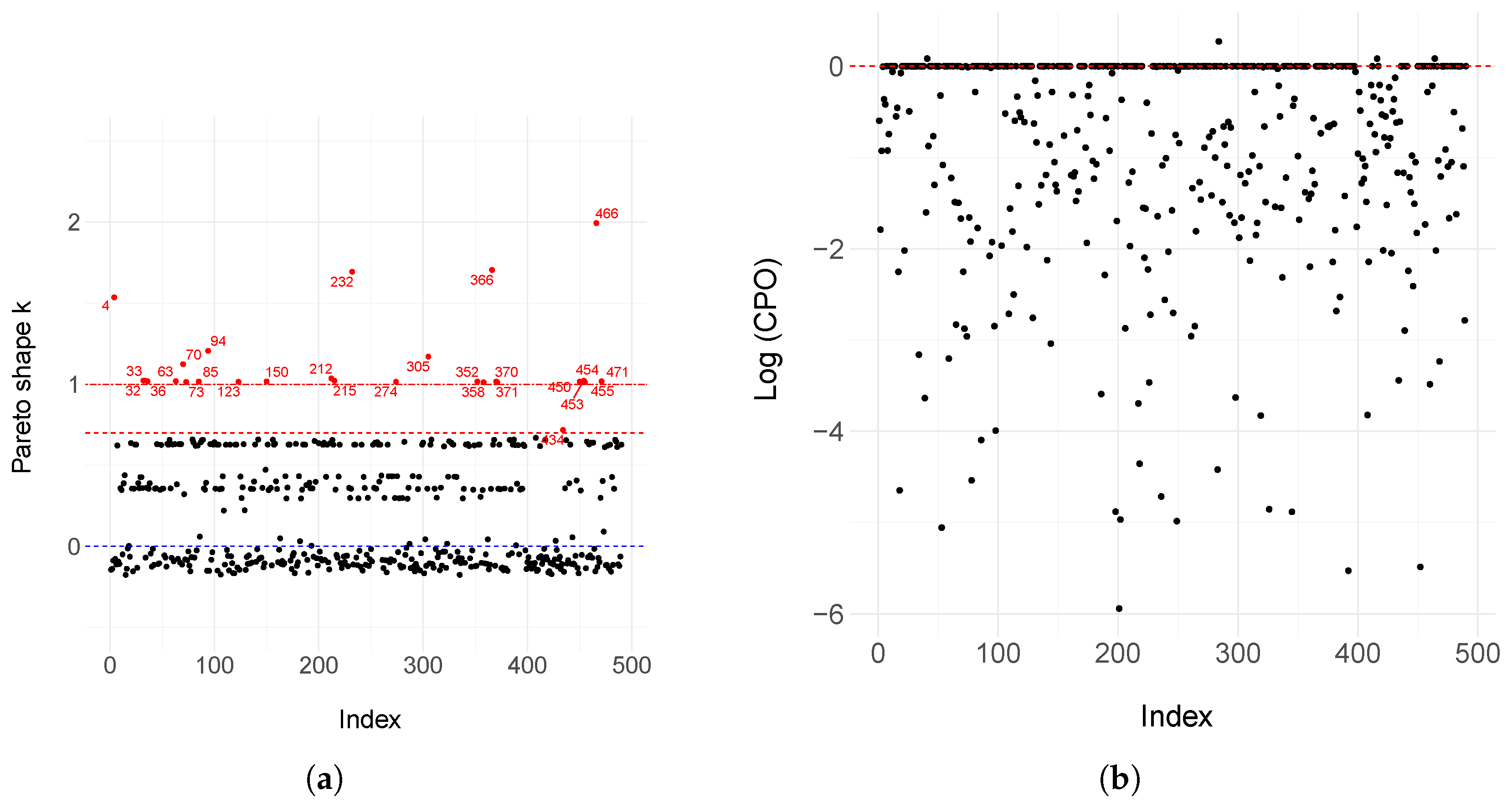
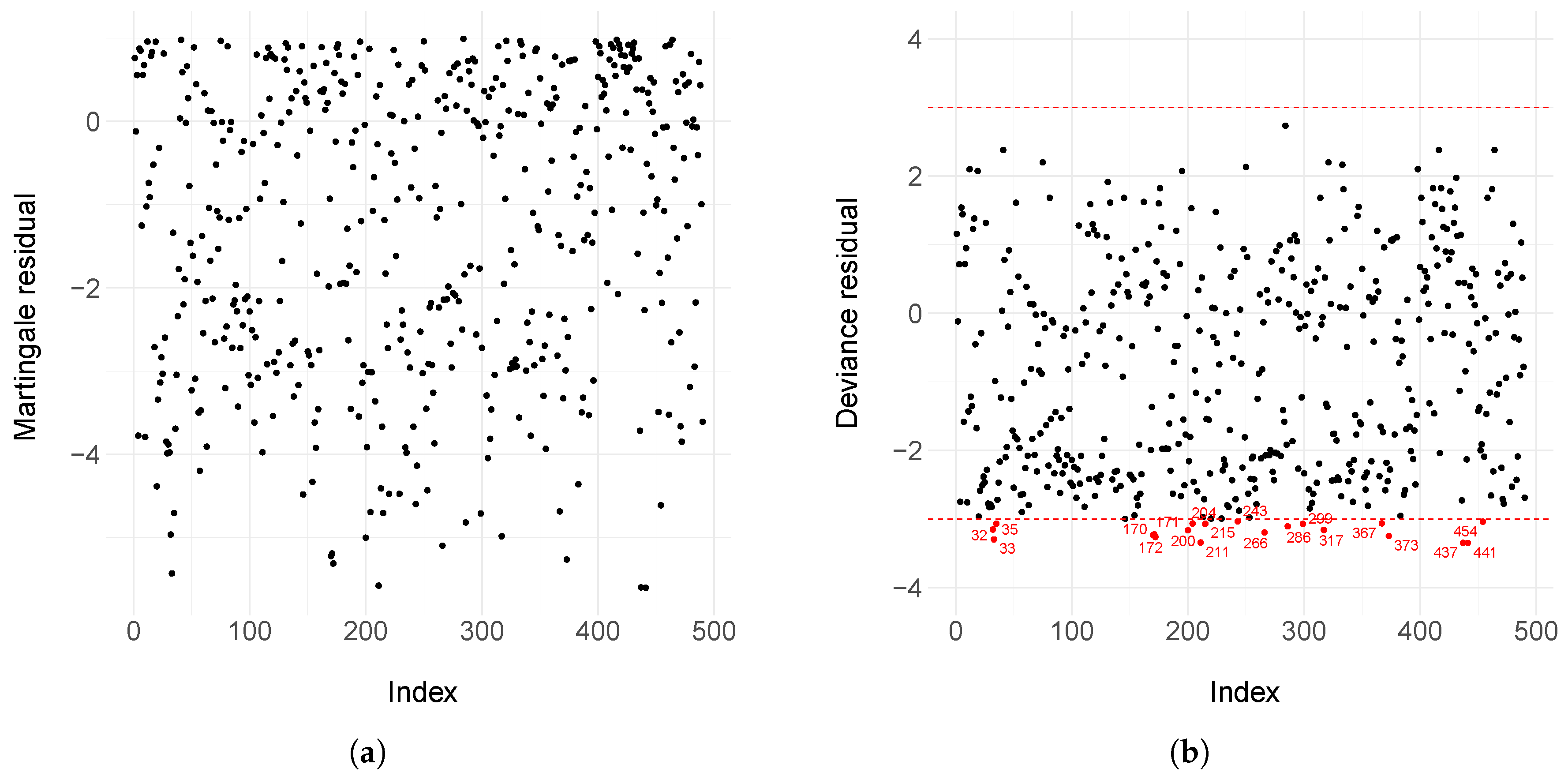
Defective models arise as alternatives to standard mixture models from a parametric perspective. A common approach in the literature is to specify the Weibull distribution for the non-cured individuals in mixed populations. In Appendix B, we present the inferential results (Table A2) and diagnostic plots (Figure A2) for the standard mixture model assuming a Weibull distribution. The model was constructed similarly to the one developed in this project, where treatments, age, and metastasis served as binary covariates to interpret the patient’s probability of cure, with regression coefficients assigned with vague priors. Upon analysis, the inferential summary revealed high standard deviations for the parameter distributions, and no statistically significant effects were observed for the factors commonly identified in the medical literature as relevant for cancer cure [39,40,41]. Additionally, the PSIS-LOO influential point diagnostics indicated high Pareto k values, with several exceeding the high (0.7) and critical (1.0) thresholds, suggesting the presence of many influential observations. Moreover, many data points showed values close to zero in terms of the logarithmic values of the CPO, indicating a loss of predictive accuracy in the standard mixture model. Finally, the deviance residuals showed that several data points had values below –3, suggesting the presence of multiple outliers in the regression model.
We believe that our Bayesian regression defective model offers substantial interpretability and practical relevance for the medical field, particularly in the context of diseases characterized by high survival rates, where advances in treatment progressively enhance patient immunity over time. Illustrative applications of this methodology include testicular cancer, prostate cancer, and thyroid cancer, among others. The regression model we propose distinguishes itself by parsimoniously employing the cure parameter to construct the survival and probability density functions that form the core of the likelihood function. Importantly, the proposed formulation is flexible and is identifiable, remains parsimonious, and provides straightforward interpretation. Our key contribution lies in integrating defective distributions into a unified framework that accommodates both cure and non-cure scenarios, thereby enabling the modeling of settings with potentially high cure probabilities and offering a novel perspective within the study of defective distributions.

5. Conclusions

In this study, we aimed to demonstrate how hospital-based intervention factors can contribute valuable information regarding the probability of cure for patients with uterine cancer in Brazil. Our Bayesian defective regression model has shown important interpretative results, pointing out age, presence of metastasis, and even chemotherapy treatment as risk factors for the probability of cure. Due to its effect and significance, surgical intervention is highly recommended to increase the probability of immunity over the years for women previously diagnosed with uterine cancer.
The statistical model discussed in this work for long-term survival data is based on a reparameterization of the defective generalized Gompertz distribution. This reparameterization was designed to provide, within studies in which the medical literature indicates a substantial probability of cured individuals, a framework for assessing risk and protective factors associated with the probability of cure among long-term survivors. While similar proposals have already been explored in standard mixture models, they often lead to unstable estimation procedures, as in well-known semiparametric versions such as the Weibull distribution, illustrated in Appendix B.
In addition, the Bayesian framework adopted here provides a coherent and flexible approach for incorporating expert medical knowledge into the modeling process, particularly through the use of informative priors on the regression coefficients associated with the cure parameter. This feature allows the model to formally integrate prior evidence on risk and protective factors related to disease progression and long-term survival.
We have also demonstrated that our estimation procedure, based on HMC-NUTS sampling, accurately recovers the true parameter values in simulation studies, while exhibiting key advantages in real-world applications by identifying statistically significant cure-related factors consistent with the medical literature. Our Bayesian model achieved a good fit to the real-world dataset and offered a more interpretable alternative compared to traditional mixture cure models commonly based on the Weibull distribution.
Additionally, the available dataset includes geographic information on patient location, which could be of particular interest for assessing whether spatial distribution influences the probability of cure. Incorporating spatial structures into the regression framework represents a promising avenue for future research. Other projects could include the defective regression model in terms of risk and protective factors on the probability of cure in scenarios such as competitive risks, multi-state, other censoring mechanisms (left or interval), and truncation.

Author Contributions

Conceptualization, D.S.-N. and V.L.T.; methodology, D.S.-N. and F.L.-N.; software, D.S.-N.; validation, D.S.-N., F.L.-N. and V.L.T.; formal analysis, D.S.-N.; investigation, D.S.-N.; resources, F.L.-N.; data curation, D.S.-N.; writing—original draft preparation, D.S.-N.; writing—review and editing, D.S.-N., F.L.-N. and V.L.T.; visualization, D.S.-N. and F.L.-N.; supervision, V.L.T. and F.L.-N.; project administration, V.L.T.; funding acquisition, V.L.T. All authors have read and agreed to the published version of the manuscript.

Funding

This research was supported by FAPESP (Fundação de Amparo à Pesquisa do Estado de São Paulo) under grant number 24/07832-6. This reseach was also carried out using the computational resources of the Center for Mathematical Sciences Applied to Industry (CeMEAI) funded by FAPESP (grant 2013/07375-0).

Data Availability Statement

The dataset provided by FOSP is available on the official website of the institution at https://fosp.saude.sp.gov.br/fosp/diretoria-adjunta-de-informacao-e-epidemiologia/rhc-registro-hospitalar-de-cancer/banco-de-dados-do-rhc/, accessed on 15 April 2025. It contains numerous clinical cases of cancer patients in the state of São Paulo. For the specific spatial and temporal scope used in this study, the processed data and analysis code can be accessed at https://github.com/Dionisioneto/Code-for-papers/tree/main/reparametrized_generalized_gompertz_for_cure_factors, accessed on 14 July 2025.

Acknowledgments

The authors thank the Fundação Oncocentro de São Paulo (FOSP) for providing the women uterine cancer dataset.

Conflicts of Interest

The authors declare no conflicts of interest.

Abbreviations

The following abbreviations are used in this manuscript:
DGGDDefective generalized Gompertz distribution
HIVHuman Immunodeficiency Virus
CDFCumulative distribution function
HMCHamiltonian Monte Carlo
MCMCMarkov Chain Monte Carlo
NUTSNo U-Turn Sampler
JAGSJust Another Gibbs Sampling
FOSPFundação Oncocentro de São Paulo
HCRHospital Cancer Registry
PSIS-LOOPareto-smoothed importance sampling - Leave one out
LPLMlogarithm pseudo marginal likelihood
DICDeviance information criterion
CPOConditional predictive ordinate

Appendix A. Model Estimation of the Defective Generalized Gompertz Distribution After Removing Influential and Outlier Observations

Table A1. Estimated values of mean, standard deviation (SD), and 95% credibility interval for uterine cancer data for the defective generalized Gompertz regression model without influential and outliers observations.
Removed DataParameterMeanSDC.I (95%)
{212}Intercept−1.39731.0447[−4.0915; −0.2253]
Age > 50−1.41420.4432[−2.5678; −0.7467]
Metastasis−1.47290.9731[−3.9467; 0.0110]
Surgery1.91750.7386[ 1.0389; 3.8880]
Chemotherapy−0.73970.4043[−1.7157; −0.1142]
Hormone therapy9.77835.0341[ 2.3046; 21.0769]
α −0.13620.0658[−0.2575; −0.0293]
ψ 0.70240.0807[ 0.5494; 0.8641]
{284}Intercept−1.39751.1653[−4.9232; −0.2421]
Age > 50−1.39990.5414[−2.9091; −0.7272]
Metastasis−1.47431.1478[−4.4371; 0.0222]
Surgery1.94700.8836[ 1.0640; 4.6306]
Chemotherapy−0.73300.4974[−2.2284; −0.0753]
Hormone therapy2.57611.6771[−0.4502; 6.2489]
α −0.14420.0666[−0.2691; −0.0240]
ψ 0.72360.0824[ 0.5736; 0.8894]
{212, 284}Intercept−1.10270.7712[−3.5164; −0.1631]
Age > 50−1.36090.3817[−2.3544; −0.7670]
Metastasis−1.32180.9824[−3.5103; 0.0167]
Surgery1.74560.5600[ 1.0238; 3.3169]
Chemotherapy−0.69670.3837[−1.7032; −0.1046]
Hormone therapy9.77215.2371[ 2.2277; 21.9298]
α −0.15440.0615[−0.2693; −0.0379]
ψ 0.73440.0794[ 0.5900; 0.8948]

Appendix B. Model Estimation and Diagnostic Assessment for the Weibull Cure Rate Model

Table A2. Estimated values of mean, standard deviation (SD), and 95% credibility interval for uterine cancer data of the Weibull mixture cure model, with shape λ and rate α parameters.
ParameterMeanSDC.I (95%)
Intercept14.41956.3232[4.6634; 28.5369]
Age > 505.16427.6398[−8.3597; 21.6942]
Metastasis2.23848.6642[−13.5450; 19.8782]
Surgery4.87697.6505[−8.8583; 21.2047]
Chemotherapy4.64167.7020[−9.3570; 20.9949]
Hormone therapy2.70958.3540[−12.0451; 20.5551]
λ 1.58330.1250[1.3493; 1.8399]
α 0.83360.0399[0.7560; 0.9142]
Figure A1. Diagnostic plot of the Pareto shape parameters k obtained from the PSIS-LOO approximation (a), and logarithm of conditional predictive ordinate (CPO) values (b), based on the Weibull mixture cure model fitted to the uterine cancer dataset.
Mca 30 00093 g0a1
Figure A2. Martingale residuals (a) and deviance residuals (b) based on the Weibull mixture cure model fitted to the uterine cancer dataset.
Mca 30 00093 g0a2

Appendix C. Model Selection Criteria in Bayesian Models

Let y i denote the complete dataset except for the i -observation ( i = 1 , , n ), the CPO for the i -th observation ( CPO i ) emerges as the posterior harmonic mean of the i -th observed likelihood:
CPO i = p ( y i y ( i ) ) = p ( y i ϑ ) p ( ϑ y ( i ) ) d ϑ = p ( y i ϑ ) j i p ( y j ϑ ) p ( ϑ ) j i p ( y j ϑ ) p ( ϑ ) d ϑ d ϑ = p ( y ) j i p ( y j ϑ ) p ( ϑ ) d ϑ p ( y ϑ ) p ( ϑ ) d ϑ = j i p ( y j ϑ ) p ( ϑ ) p ( y ) d ϑ 1 = p ( y i ϑ ) j i p ( y j ϑ ) p ( ϑ ) p ( y i ϑ ) p ( y ( i ) ) d ϑ 1 = 1 p ( y i ϑ ) p ( ϑ y ) d ϑ 1 .
The Equation (A1) shows that it is possible to perform cross validation without a separate analyses. Using MCMC samples, we can estimate the individual CPO as
CPO i ^ = 1 n k = 1 n 1 p ( y i ϑ k ) 1 ,
where ϑ k is the k -th sampled parameter vector from an MCMC analysis from the sampled posterior distribution ( k = 1 , , K ) [42]. The quantity p ( y i ϑ k ) is generally only available on the log scale, therefore, we have the convenient formula
log CPO i ^ = log ( n ) + l i , m i n log k = 1 n exp { l i , m i n l i , k } ,
where l i , k = log ( p ( y i ϑ k ) ) is the observed likelihood for the i -th observation using the k -th sampled parameter vector, and l i , m i n = m i n { l i , k : k = 1 , , n } .
The logarithm of pseudomarginal likelihood (LPML) is estimated by sum of the individual CPO values:
LPML = i = 1 n log CPO i ^ .
The Deviance Information Criterion (DIC) is another measure to compare Bayesian models, which penalizes the model fitting based on complexity [43]. The DIC can be expressed as
D ( ϑ ) = 2 i = 1 n log f ( y i ϑ ) ,
where f ( . ) is the probability density function of the defective model under evaluation. The posterior mean of D ( ϑ ) can be estimated from samples of posterior distribution. Indeed, D ¯ = k = 1 K D ( ϑ k ) , where the ϑ k is the k -th posterior sample. According to [43], the DIC is estimated as
D I C ^ = D ¯ + 1 2 p D ,
where p D = D ¯ D ( ϑ ¯ ) is the effective parameters numbers, and D ( ϑ ¯ ) = 2 log ( p ( y ϑ ¯ ) ) is the deviance evaluated at the posterior mean of the parameters, where ϑ ¯ is typically the posterior mean vector of parameters.
To improve the accuracy and stability of leave-one-out (LOO) cross-validation estimates, we employ Pareto Smoothed Importance Sampling (PSIS) as proposed by [44]. This method regularizes the distribution of importance sampling weights by smoothing extreme values that often arise in Bayesian models, particularly when importance ratios exhibit heavy-tailed behavior.
Importance sampling is known to be sensitive to extreme weights, which can result in unstable and high-variance estimates. PSIS mitigates this issue by fitting a generalized Pareto distribution (GPD) to the upper tail of the distribution, specifically, the top 20% of the importance ratios. The fitted shape parameter k ^ serves as a diagnostic measure for assessing the reliability of the estimates. This approach builds on and extends earlier diagnostic tools developed by [45,46].
To obtain the PSIS values for each individual, we follows the steps:
(i)
For each data point i, i = 1 , , n , a GPD is fitted to the largest 20% of the importance weights
r i s = 1 p ( y i ϑ s ) p ( ϑ s y i ) p ( ϑ s y ) .
This is done independently for each observation using empirical Bayes estimation;
(ii)
The M largest weights are replaced by their expected order statistics from the fitted GPD, using the inverse cumulative distribution function
F 1 z 1 / 2 M , z = 1 , , M .
where M is the number of simulation draws used to fit the Pareto (in this case, M = 0.2 S ). This results in a smoothed set of weights w ˜ s i , indexed by simulation draws s and data points i;
(iii)
To guarantee finite variance of the estimate, the stabilized weights are truncated at S 3 / 4 w ¯ i , where w ¯ i is the average of the smoothed weights for observation i. The final truncated weights are denoted by w s i .
The above steps are repeated for each observation ( i = 1 , , n ), to get the vector of weights w i s , s = 1 , , S , for each i = 1 , , n . The weights should present a better behavior than the raw importance rations r i s .
The results can then be combined to compute the desired LOO estimates. The PSIS is based on the −2 times the value of the expected log pointwise predictive density given by
elpd ^ psis-loo = i = 1 n log s = 1 S w i s p ( y i θ s ) s = 1 S w i s .
For the individual values of k ^ of the generalized Pareto distribution, ref. [44] guarantee reliable estimates under the central limit theorem for k ^ . If the estimated tail shape parameter k ^ exceeds 0.5 but is less than 0.7, the estimation the generalized central limit theorem for stable distributions holds. If k ^ > 0.7 , the approximation is not reliable and it is an evidence of influential data point in the Bayesian model. If k ^ > 1.0 , the variance and the mean of the raw ratios distribution do not exist and it affects directly the estimation of PSIS-LOO, indicating poor predictive performance [44].

References

  1. Campos, L.N.; César, C.C.; Guimarães, M.D.C. Quality of life among HIV-infected patients in Brazil after initiation of treatment. Clinics 2009, 64, 867–875. [Google Scholar] [CrossRef] [PubMed]
  2. Bourke, L.; Boorjian, S.A.; Briganti, A.; Klotz, L.; Mucci, L.; Resnick, M.J.; Rosario, D.J.; Skolarus, T.A.; Penson, D.F. Survivorship and improving quality of life in men with prostate cancer. Eur. Urol. 2015, 68, 374–383. [Google Scholar] [CrossRef] [PubMed]
  3. Sugimura, H.; Yang, P. Long-term survivorship in lung cancer: A review. Chest 2006, 129, 1088–1097. [Google Scholar] [CrossRef] [PubMed]
  4. Vasan, N.; Baselga, J.; Hyman, D.M. A view on drug resistance in cancer. Nature 2019, 575, 299–309. [Google Scholar] [CrossRef]
  5. Boag, J.W. Maximum likelihood estimates of the proportion of patients cured by cancer therapy. J. R. Stat. Soc. Ser. B (Methodol.) 1949, 11, 15–53. [Google Scholar] [CrossRef]
  6. Berkson, J.; Gage, R.P. Survival curve for cancer patients following treatment. J. Am. Stat. Assoc. 1952, 47, 501–515. [Google Scholar] [CrossRef]
  7. Lambert, P.C. Modeling of the cure fraction in survival studies. Stata J. 2007, 7, 351–375. [Google Scholar] [CrossRef]
  8. Mazucheli, J.; Coelho-Barros, E.A.; Achcar, J.A. The exponentiated exponential mixture and non-mixture cure rate model in the presence of covariates. Comput. Methods Programs Biomed. 2013, 112, 114–124. [Google Scholar] [CrossRef]
  9. Balka, J.; Desmond, A.F.; McNicholas, P.D. Review and implementation of cure models based on first hitting times for Wiener processes. Lifetime Data Anal. 2009, 15, 147–176. [Google Scholar] [CrossRef]
  10. Rocha, R.; Nadarajah, S.; Tomazella, V.; Louzada, F. Two new defective distributions based on the Marshall–Olkin extension. Lifetime Data Anal. 2016, 22, 216–240. [Google Scholar] [CrossRef]
  11. Rocha, R.; Nadarajah, S.; Tomazella, V.; Louzada, F.; Eudes, A. New defective models based on the Kumaraswamy family of distributions with application to cancer data sets. Stat. Methods Med. Res. 2017, 26, 1737–1755. [Google Scholar] [CrossRef]
  12. Vieira Tojeiro, C.A.; Tomazella, V.; Jerez-Lillo, N.; Ramos, P.L. The Defective Beta-Gompertz Distribution for Cure Rate Regression Models. J. Stat. Theory Pract. 2025, 19, 19. [Google Scholar] [CrossRef]
  13. El-Gohary, A.; Alshamrani, A.; Al-Otaibi, A.N. The generalized Gompertz distribution. Appl. Math. Model. 2013, 37, 13–24. [Google Scholar] [CrossRef]
  14. Mudholkar, G.S.; Srivastava, D.K.; Freimer, M. The exponentiated Weibull family: A reanalysis of the bus-motor-failure data. Technometrics 1995, 37, 436–445. [Google Scholar] [CrossRef]
  15. Nadarajah, S.; Gupta, A.K. The exponentiated gamma distribution with application to drought data. Calcutta Stat. Assoc. Bull. 2007, 59, 29–54. [Google Scholar] [CrossRef]
  16. Gupta, R.D.; Kundu, D. Theory & methods: Generalized exponential distributions. Aust. New Zealand J. Stat. 1999, 41, 173–188. [Google Scholar] [CrossRef]
  17. Rodrigues, A.; Borges, P.; Santos, B. A defective cure rate quantile regression model for male breast cancer data. J. Appl. Stat. 2024, 52, 1485–1512. [Google Scholar] [CrossRef]
  18. Lehmann, E.L. The Power of Rank Tests. Ann. Math. Stat. 1953, 24, 23–43. [Google Scholar] [CrossRef]
  19. Gelman, A.; Carlin, J.B.; Stern, H.S.; Rubin, D.B. Bayesian Data Analysis; Chapman and Hall/CRC: New York, NY, USA, 1995. [Google Scholar]
  20. de Castro, M.; Gómez, Y.M. A Bayesian cure rate model based on the power piecewise exponential distribution. Methodol. Comput. Appl. Probab. 2020, 22, 677–692. [Google Scholar] [CrossRef]
  21. dos Santos Junior, P.C.; Schneider, S. Power piecewise exponential model for interval-censored data. J. Stat. Theory Pract. 2022, 16, 26. [Google Scholar] [CrossRef]
  22. Metropolis, N.; Rosenbluth, A.W.; Rosenbluth, M.N.; Teller, A.H.; Teller, E. Equation of state calculations by fast computing machines. J. Chem. Phys. 1953, 21, 1087–1092. [Google Scholar] [CrossRef]
  23. Hastings, W.K. Monte Carlo sampling methods using Markov chains and their applications. Biometrika 1970, 57, 97–109. [Google Scholar] [CrossRef]
  24. Geman, S.; Geman, D. Stochastic relaxation, Gibbs distributions, and the Bayesian restoration of images. IEEE Trans. Pattern Anal. Mach. Intell. 1984, 6, 721–741. [Google Scholar] [CrossRef] [PubMed]
  25. Neal, R.M. MCMC using Hamiltonian dynamics. Handb. Markov Chain Monte Carlo 2011, 2, 2. [Google Scholar]
  26. Duane, S.; Kennedy, A.D.; Pendleton, B.J.; Roweth, D. Hybrid Monte Carlo. Phys. Lett. B 1987, 195, 216–222. [Google Scholar] [CrossRef]
  27. Stan Development Team. RStan: The R Interface to Stan, R package version 2.32.7. 2025. Available online: https://mc-stan.org/ (accessed on 25 May 2025).
  28. Betancourt, M.; Byrne, S.; Livingstone, S.; Girolami, M. The geometric foundations of Hamiltonian Monte Carlo. Bernoulli 2017, 23, 2257–2298. [Google Scholar] [CrossRef]
  29. Hoffman, M.D.; Gelman, A. The No-U-Turn sampler: Adaptively setting path lengths in Hamiltonian Monte Carlo. J. Mach. Learn. Res. 2014, 15, 1593–1623. [Google Scholar]
  30. Monnahan, C.C.; Thorson, J.T.; Branch, T.A. Faster estimation of Bayesian models in ecology using Hamiltonian Monte Carlo. Methods Ecol. Evol. 2017, 8, 339–348. [Google Scholar] [CrossRef]
  31. Astfalck, L.; Hodkiewicz, M. Hamiltonian Monte Carlo sampling for Bayesian hierarchical regression in prognostics. PHM Soc. Asia Pac. Conf. 2017, 1. [Google Scholar] [CrossRef]
  32. Therneau, T.M.; Grambsch, P.M.; Fleming, T.R. Martingale-based residuals for survival models. Biometrika 1990, 77, 147–160. [Google Scholar] [CrossRef]
  33. Pather, S.; O’Leary, M.; Carter, J. Endometrial cancer and its management. Women’S Health 2007, 3, 45–54. [Google Scholar] [CrossRef]
  34. Jemal, A.; Tiwari, R.C.; Murray, T.; Ghafoor, A.; Samels, A.; Ward, E.; Feuer, E.J.; Thun, M.J. Cancer statistics, 2004. CA Cancer J. Clin. 2004, 54, 8–29. [Google Scholar] [CrossRef]
  35. Parkin, D.M.; Pisani, P.; Ferlay, J. Global cancer statistics. CA Cancer J. Clin. 1999, 49, 33–64. [Google Scholar] [CrossRef]
  36. Major, F.J.; Blessing, J.A.; Silverberg, S.G.; Morrow, C.P.; Creasman, W.T.; Currie, J.L.; Yordan, E.; Brady, M.F. Prognostic factors in early-stage uterine sarcoma: A gynecologic oncology group study. Cancer 1993, 71 (Suppl. S4), 1702–1709. [Google Scholar] [CrossRef] [PubMed]
  37. Giuntoli, R.L.; Metzinger, D.S.; DiMarco, C.S.; Cha, S.S.; Sloan, J.A.; Keeney, G.L.; Gostout, B.S. Retrospective review of 208 patients with leiomyosarcoma of the uterus: Prognostic indicators, surgical management, and adjuvant therapy. Gynecol. Oncol. 2003, 89, 460–469. [Google Scholar] [CrossRef] [PubMed]
  38. Vehtari, A.; Gelman, A.; Gabry, J. Practical Bayesian model evaluation using leave-one-out cross-validation and WAIC. Stat. Comput. 2017, 27, 1413–1432. [Google Scholar] [CrossRef]
  39. Boggess, J.F.; Kilgore, J.E.; Tran, A.-Q. Uterine cancer. In Abeloff’s Clinical Oncology; Elsevier: Amsterdam, The Netherlands, 2020; pp. 1508–1524. [Google Scholar]
  40. Green, J.A.; Kirwan, J.M.; Tierney, J.F.; Symonds, P.; Fresco, L.; Collingwood, M.; Williams, C.J. Survival and recurrence after concomitant chemotherapy and radiotherapy for cancer of the uterine cervix: A systematic review and meta-analysis. Lancet 2001, 358, 781–786. [Google Scholar] [CrossRef]
  41. Lee, N.K.; Cheung, M.K.; Shin, J.Y.; Husain, A.; Teng, N.N.; Berek, J.S.; Kapp, D.S.; Osann, K.; Chan, J.K. Prognostic factors for uterine cancer in reproductive-aged women. Obstet. Gynecol. 2007, 109, 655–662. [Google Scholar] [CrossRef]
  42. Chen, M.-H.; Ibrahim, J.G. Bayesian predictive inference for time series count data. Biometrics 2000, 56, 678–685. [Google Scholar] [CrossRef]
  43. Spiegelhalter, D.J.; Best, N.G.; Carlin, B.P.; Van Der Linde, A. Bayesian measures of model complexity and fit. J. R. Stat. Soc. Ser. B (Stat. Methodol.) 2002, 64, 583–639. [Google Scholar] [CrossRef]
  44. Vehtari, A.; Gelman, A.; Gabry, J. Efficient implementation of leave-one-out cross-validation and WAIC for evaluating fitted Bayesian models. arXiv 2015, arXiv:1507.04544. [Google Scholar]
  45. Peruggia, M. On the variability of case-deletion importance sampling weights in the Bayesian linear model. J. Am. Stat. Assoc. 1997, 92, 199–207. [Google Scholar] [CrossRef]
  46. Epifani, I.; MacEachern, S.N.; Peruggia, M. Case-deletion importance sampling estimators: Central limit theorems and related results. Electron. J. Stat. 2008, 2, 774–806. [Google Scholar] [CrossRef]
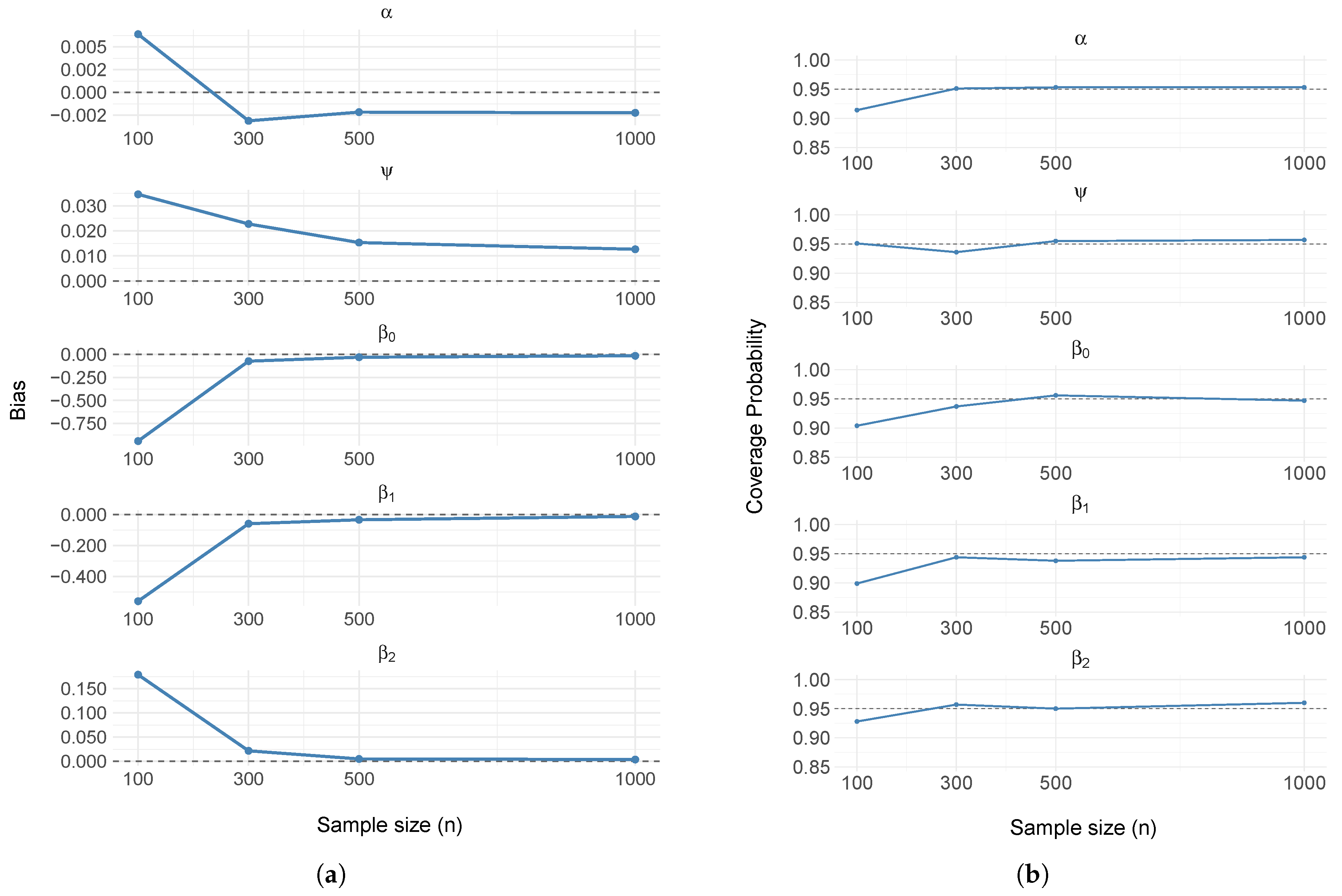
Figure 1. Bias (a) and coverage probability (b) for simulated data from the defective generalized Gompertz model per sample size.
Mca 30 00093 g001
Figure 2. Kaplan–Meier curve with 95% confidence interval of patients with uterine cancer.
Mca 30 00093 g002
Figure 3. Diagnostic plot of the Pareto shape parameters k obtained from the PSIS-LOO approximation (a), and conditional predictive ordinate (CPO) values (b), based on the DGGD fitted to the uterine cancer dataset.
Mca 30 00093 g003
Figure 4. Martingale residuals (a) and deviance residuals (b) based on the defective generalized Gompertz model fitted to the uterine cancer dataset.
Mca 30 00093 g004
Table 1. Estimated values of mean, standard deviation (SD), and 95% credibility interval for uterine cancer data using the DGGD.
ParameterMeanSDC.I (95%)
Intercept−1.36251.0914[−5.0000; −0.2572]
Age > 50−1.33330.4675[−2.6774; −0.7029]
Metastasis−1.48991.2310[−5.5832; 0.0135]
Surgery1.88000.8130[ 1.0414; 4.4872]
Chemotherapy−0.69780.4699[−1.9691; −0.0611]
Hormone Therapy2.62241.6631[−0.3416; 6.3090]
α −0.14450.0641[−0.2648; −0.0246]
ψ 0.71110.0789[ 0.5616; 0.8709]
Table 2. Values of DIC, PSIS-LOO, and −2*LPML for generalized Gompertz and Gompertz defective regression models for uterine cancer dataset.
ModelDICPSIS-LOO−2*LPLM
Generalized Gompertz1315.761325.421325.44
Gompertz1328.691331.401331.59
Disclaimer/Publisher’s Note: The statements, opinions and data contained in all publications are solely those of the individual author(s) and contributor(s) and not of MDPI and/or the editor(s). MDPI and/or the editor(s) disclaim responsibility for any injury to people or property resulting from any ideas, methods, instructions or products referred to in the content.