High-Performance Simulation of Generalized Tempered Stable Random Variates: Exact and Numerical Methods for Heavy-Tailed Data

Abstract

The Generalized Tempered Stable (GTS) distribution extends classical stable laws through exponential tempering, preserving the power-law behavior while ensuring finite moments. This makes it especially suitable for modeling heavy-tailed financial data. However, the lack of closed-form densities poses significant challenges for simulation. This study provides a comprehensive and systematic comparison of GTS simulation methods, including rejection-based algorithms, series representations, and an enhanced Fast Fractional Fourier Transform (FRFT)-based inversion method. Through extensive numerical experiments on major financial assets (Bitcoin, Ethereum, the S&P 500, and the SPY ETF), this study demonstrates that the FRFT method outperforms others in terms of accuracy and ability to capture tail behavior, as validated by goodness-of-fit tests. Our results provide practitioners with robust and efficient simulation tools for applications in risk management, derivative pricing, and statistical modeling.

1. Introduction

In many areas of applied statistics and data analysis—particularly in finance, insurance, and environmental modeling—empirical data often exhibit heavy tails, skewness, and discontinuous jumps that deviate significantly from Gaussian assumptions [1,2,3]. Classical models based on normal distributions frequently fail to capture these features, especially when modeling extreme events or tail risks [4].

The Generalized Tempered Stable (GTS) distribution has emerged as a flexible and powerful framework for modeling such phenomena. By introducing exponential tempering to the Lévy measure, it extends classical stable distributions while preserving their heavy-tailed behavior and ensuring finite moments [5,6]. These properties make GTS distributions particularly valuable for modeling Lévy processes with jump activity in financial applications [7]. Moreover, the GTS family encompasses several notable special cases [6,8,9,10,11], further highlighting its flexibility and relevance across various applications.

Despite their theoretical appeal, simulating GTS random variates remains a challenging task. The absence of closed-form probability densities precludes the use of standard techniques that rely on explicit cumulative distribution evaluations [12]. In practice, simulation from the GTS distribution is essential for conducting Monte Carlo experiments, performing risk assessments, fitting models to data, and generating synthetic datasets for testing algorithms [13].

To address this challenge, several approaches have been developed, including rejection-based algorithms (e.g., Standard Stable Rejection, Double Rejection, and Two-Dimensional Single Rejection) [12,14,15,16,17], series representations (e.g., Shot Noise and Inverse Tail Integral methods) [5,18,19], and inversion-based techniques leveraging the characteristic function [1,20]. While each has advantages, they also face limitations in efficiency, accuracy, or robustness—particularly when applied to financial assets with very small stability indices or extreme tempering parameters (${\beta }_{\pm }\to 0$, ${\lambda }_{\pm }\to +\infty$). Moreover, the literature lacks a systematic empirical comparison of these methods under realistic, data-driven conditions.

This paper aims to fill that gap by providing a comprehensive review, implementation, and empirical evaluation of simulation methods for GTS random variates. We categorize the algorithms into exact methods (rejection-based) and numerical approaches (series representations and inversion techniques). Our key contributions are as follows:

1.

Systematic Empirical Benchmarking: We perform an extensive numerical study using high-frequency daily return data from major financial assets (Bitcoin, Ethereum, S&P 500, SPY ETF), whose parameters often push simulation methods to their limits. This provides a realistic benchmark absent in purely theoretical comparisons.

2.

Implementation and Analysis of Exact Methods: We implement and evaluate key rejection-based algorithms (Standard Stable Rejection, Double Rejection, Two-Dimensional Single Rejection), providing a clear analysis of their computational complexity and identifying their breaking points, particularly for equity indices with extremely low stability index values.

3.

Implementation and Analysis of Series Representations: We investigate the inverse Lévy measure and Shot Noise series representation methods, demonstrating their theoretical elegance but also their practical limitations and sensitivity to parameter values.

4.

An Enhanced FRFT-Based Inversion Framework: We propose and implement an advanced numerical inversion method that leverages the characteristic function of the GTS distribution, combining [21] a Fast Fractional Fourier Transform (FRFT) and Newton–Cotes quadrature. This method achieves high accuracy and robustness across parameter regimes, addressing key shortcomings of rejection and series methods.

5.

Rigorous Validation: Beyond visual Q-Q plot analysis, we use statistical goodness-of-fit tests (Kolmogorov–Smirnov and Anderson–Darling) to assess the fidelity of each method, with a particular focus on tail behavior.

Our results show that the enhanced FRFT-based inversion method consistently outperforms existing techniques in both accuracy and robustness. This establishes it as a practical and reliable tool for applications in risk management, derivative pricing, and statistical modeling where accurate reproduction of heavy-tailed dynamics is essential.

The remainder of this paper is structured as follows: Section 2 reviews the mathematical foundations of GTS distributions. Section 3, Section 4, Section 5, Section 6 and Section 7 present the simulation algorithms. Section 8.2 reports empirical results and comparisons. Section 9 concludes with practical recommendations and directions for future research.

2. Generalized Tempered Stable (GTS) Distribution

The Generalized Tempered Stable (GTS) distribution is a family of infinitely divisible distributions that generalizes the classical stable laws by introducing exponential tempering into the Lévy measure. This modification preserves the power-law behavior in the central part of the distribution while damping the tails, ensuring the existence of moments and improving the tractability of the model in applications.

Formally, a random variable $X\sim GTS({\beta }_{+},{\beta }_{-},{\alpha }_{+},{\alpha }_{-},{\lambda }_{+},{\lambda }_{-})$ has a Lévy measure $V\left(dx\right)$ given by

$$V\left(dx\right)=\left[{\alpha }_{+}{\displaystyle \frac{e^{-{\lambda }_{+}x}}{x^{1+{\beta }_{+}}}}{\mathbf{1}}_{\{x>0\}}+{\alpha }_{-}{\displaystyle \frac{e^{-{\lambda }_{-}\left|x\right|}}{{\left|x\right|}^{1+{\beta }_{-}}}}{\mathbf{1}}_{\{x<0\}}\right]dx,$$

(1)

where

• ${\beta }_{+},{\beta }_{-}\in (0,1)$ are stability index parameters, controlling the heaviness of the tails on the positive and negative axes, respectively;
• ${\alpha }_{+},{\alpha }_{-}>0$ are scale parameters, determining the overall intensity of jumps;
• ${\lambda }_{+},{\lambda }_{-}>0$ are tempering parameters, governing the exponential decay of large jumps in either direction.

Remark 1.

The Lévy measure $V\left(dx\right)$ is a Borel measure on $\mathbb{R}\backslash \left\{0\right\}$ that satisfies the following condition:

• No Jump at Zero: $V\left(0\right)=0$;
• Integrability of Small Jumps: ${\int }_{\mathbb{R}}{(1\wedge |x|}^2)V\left(dx\right)<\infty$.

The importance of the Lévy measure is shown by the Lévy–Khintchine representation, which states that the characteristics of any Lévy process are uniquely defined by a triplet $(a,\sigma ,V)$, consisting of

• A drift term (a);
• A diffusion or variance coefficient (σ), which controls the continuous, Gaussian-motion component;
• The Lévy measure (V), which precisely quantifies the frequency and size of the jumps.

Thus, the triplet $(a,\sigma ,V)$ offers a unique and exhaustive signature for any Lévy process.

The activity process of the GTS distribution can be studied from the integral (2) of the Lévy measure (1):

$$\begin{array}{c}\hfill {\int }_{-\infty }^{+\infty }V\left(dx\right)=+\infty \mathrm{if}0\le {\beta }_{+}<1\wedge 0\le {\beta }_{-}<1.\end{array}$$

(2)

As shown in Equation (2), for ${\beta }_{+},{\beta }_{-}\in (0,1)$, the Lévy density ($V\left(dx\right)$) is not integrable as it goes off to infinity too rapidly as x goes to zero, due to a large number of very small jumps. The GTS distribution is described as an infinite activity process with an infinite number of jumps within any given time interval.

In addition to the infinite activities process, the variation of the process can be studied by solving the following integral [22]:

$$\begin{array}{c}\hfill {\int }_{-1}^1\left|x\right|V\left(dx\right)<+\infty \mathrm{if}0\le {\beta }_{+}<1\wedge 0\le {\beta }_{-}<1.\end{array}$$

(3)

Refer to [11] for further development of Equation (3).

As shown in Equation (3), GTS distribution is a finite variation process, and generates a type B Lévy process [23], which is a purely non-Gaussian infinite activity Lévy process of finite variation whose sample paths have an infinite number of small jumps and a finite number of large jumps in any finite time interval. In particular, being of bounded variation shows that $X\sim GTS({\beta }_{+},{\beta }_{-},{\alpha }_{+},{\alpha }_{-},{\lambda }_{+},{\lambda }_{-})$ can be written as the difference of two independent subordinators [22,24]:

$$X=X^{+}-X^{-}\mathrm{with}{X}^{+}\sim TS({\beta }_{+},{\alpha }_{+},{\lambda }_{+}),X^{-}\sim TS({\beta }_{-},{\alpha }_{-},{\lambda }_{-}),$$

(4)

where $X_{+}\sim TS({\beta }_{+},{\alpha }_{+},{\lambda }_{+})$ and $X_{-}\sim TS({\beta }_{-},{\alpha }_{-},{\lambda }_{-})$ are subordinators.

By adding a drift parameter, we have the following expression:

$$\begin{array}{c}\hfill Y=\mu +X\sim GTS(\mu ,{\beta }_{+},{\beta }_{-},{\alpha }_{+},{\alpha }_{-},{\lambda }_{+},{\lambda }_{-}).\end{array}$$

(5)

Theorem 1.

Consider a variable $Y\sim GTS(\mu ,{\beta }_{+},{\beta }_{-},{\alpha }_{+},{\alpha }_{-},{\lambda }_{+},{\lambda }_{-})$. The characteristic exponent can be written as

$$\begin{array}{cc}\hfill \psi \left(\xi \right)& =\mu \xi i+{\alpha }_{+}\mathrm{\Gamma }(-{\beta }_{+})\left({({\lambda }_{+}-i\xi )}^{{\beta }_{+}}-{{\lambda }_{+}}^{{\beta }_{+}}\right)+\hfill \\ \hfill & {\alpha }_{-}\mathrm{\Gamma }(-{\beta }_{-})\left({({\lambda }_{-}+i\xi )}^{{\beta }_{-}}-{{\lambda }_{-}}^{{\beta }_{-}}\right).\hfill \end{array}$$

(6)

See [25,26,27] for Theorem 1’s proof.

Maximum Likelihood GTS Parameter Estimation for Four Key Financial Assets

The GTS parameter estimation results for Bitcoin and Ethereum are presented in Table 1, while those for the S&P 500 index and the SPY ETF are shown in Table 2. The values in brackets represent the asymptotic standard errors, computed using the inverse of the Hessian matrix.

Table 1. GTS parameter estimation for Bitcoin and Ethereum [26].

Parameter	Bitcoin			Ethereum
	Estimate	Std Err	$\mathit{Pr}(\mathit{Z}>|\mathit{z}\left|\right)$	Estimate	Std Err	$\mathit{Pr}(\mathit{Z}>|\mathit{z}\left|\right)$
$\mu$	−0.1216	(0.375)	$7.5\times {10}^{-01}$	−0.4854	(1.008)	$6.3\times {10}^{-01}$
${\beta }_{+}$	0.3155	(0.136)	$2.0\times {10}^{-02}$	0.3904	(0.164)	$1.7\times {10}^{-02}$
${\beta }_{-}$	0.4066	(0.117)	$4.9\times {10}^{-04}$	0.4045	(0.210)	$5.4\times {10}^{-02}$
${\alpha }_{+}$	0.7477	(0.047)	$6.2\times {10}^{-56}$	0.9582	(0.106)	$1.1\times {10}^{-19}$
${\alpha }_{-}$	0.5446	(0.037)	$4.8\times {10}^{-48}$	0.8005	(0.110)	$4.2\times {10}^{-13}$
${\lambda }_{+}$	0.2465	(0.036)	$4.9\times {10}^{-12}$	0.1667	(0.029)	$1.1\times {10}^{-08}$
${\lambda }_{-}$	0.1748	(0.026)	$2.2\times {10}^{-11}$	0.1708	(0.036)	$2.5\times {10}^{-06}$

Table 2. GTS parameter estimation for S&P 500 Index and SPY ETF [26].

Parameter	S&P 500 Index			SPY ETF
	Estimate	Std Err	$\mathit{Pr}(\mathit{Z}>|\mathit{z}\left|\right)$	Estimate	Std Err	$\mathit{Pr}(\mathit{Z}>|\mathit{z}\left|\right)$
$\mu$	−0.2494	(0.208)	$2.3\times {10}^{-01}$	−0.2606	(0.135)	$5.3\times {10}^{-02}$
${\beta }_{+}$	0.3286	(0.308)	$2.9\times {10}^{-01}$	0.3408	(0.189)	$7.1\times {10}^{-02}$
${\beta }_{-}$	0.0886	(0.176)	$6.1\times {10}^{-01}$	0.0222	(0.212)	$9.2\times {10}^{-01}$
${\alpha }_{+}$	0.7924	(0.350)	$2.4\times {10}^{-02}$	0.7877	(0.225)	$4.6\times {10}^{-04}$
${\alpha }_{-}$	0.5422	(0.107)	$3.6\times {10}^{-07}$	0.5971	(0.141)	$2.4\times {10}^{-05}$
${\lambda }_{+}$	1.2797	(0.348)	$2.4\times {10}^{-04}$	1.2885	(0.226)	$1.2\times {10}^{-08}$
${\lambda }_{-}$	0.9371	(0.144)	$8.0\times {10}^{-11}$	1.0143	(0.177)	$9.4\times {10}^{-09}$

For all financial assets considered, the maximum likelihood estimates indicate that $\mu$ is negative, while other parameters are positive, as expected in the literature. However, the relatively large standard errors suggest that $\mu$ is not statistically significant at the 5% level.

As shown in Table 1 and Table 2, except for the index of stability parameters (${\beta }_{+}-{\beta }_{-}$), the tempering parameters (${\lambda }_{+}$, ${\lambda }_{-}$) and the scale parameters (${\alpha }_{+}$, ${\alpha }_{-}$) are all statistically significant at the 5% level.

Remark 2.

A comprehensive methodology for fitting the seven-parameter Generalized Tempered Stable (GTS) distribution—along with parameter estimation results—is presented in [26]. The data source and some empirical findings are summarized as follows:

• Data Sources:

  –

  Historical price data for Bitcoin (BTC) and Ethereum (ETH) were collected from CoinMarketCap. The time span covers 28 April 2013 to 4 July 2024 for BTC, and 7 August 2015 to 4 July 2024 for ETH.

  –

  Historical price data for the S&P 500 Index and the SPY ETF were obtained from Yahoo Finance, covering the period from 4 January 2010 to 22 July 2024. The prices were adjusted for stock splits and dividends.

• GTS parameter estimation: The methodology for estimating the seven parameters using the Enhanced Fast Fractional Fourier Transform (FRFT) has been extensively developed in [26,28,29,30,31], providing a comprehensive approach for fitting the rich class of GTS distributions.
• Model Comparison: Based on log-likelihood, Akaike Information Criterion (AIC), and Bayesian Information Criterion (BIC), the seven-parameter GTS distribution outperforms the classical two-parameter normal distribution (Geometric Brownian Motion, GBM).
• Goodness-of-Fit Tests: The Kolmogorov–Smirnov, Anderson–Darling, and Pearson chi-squared tests confirm the superior fit of the GTS model, especially in capturing heavy tails and asymmetries in return distributions.
• Benchmarking Against Alternative Models: The GTS distribution demonstrates improved empirical performance over

  –

  The KoBoL distribution ($\beta ={\beta }_{+}={\beta }_{-}$);

  –

  The Carr–Geman–Madan–Yor (CGMY) model ($\lambda ={\lambda }_{+}={\lambda }_{-}$ and $\beta ={\beta }_{+}={\beta }_{-}$);

  –

  The Bilateral Gamma distribution (${\beta }_{+}={\beta }_{-}=0$).

3. β-Stable Distributions and Simulation Algorithms

3.1. $\beta$-Stable Distributions: Review

We consider the class of all stable distributions with four parameters $(\beta ,\delta ,\sigma ,\mu )$, denoted by $S_{\beta }(\sigma ,\delta ,\mu )$. $X\in S_{\beta }(\sigma ,\delta ,\mu )$ means that X is a stable random variable (r.v) with parameters $(\beta ,\delta ,\sigma ,\mu )$. $S_{\beta }(\sigma ,\delta ,\mu )$ is the notation used in [2]. In the literature, various notational conventions are commonly used; for instance, the parameterization $S(\beta ,\delta ,\sigma ,\mu )$ is employed in [4]. A random variable X is said to have a stable distribution, $X\in S_{\beta }(\sigma ,\delta ,\mu )$, if and only if the logarithm of its characteristic function $\psi \left(\xi \right)$ has the following canonical form [32,33,34]:

$$\begin{array}{c}\hfill Log\left(\psi \left(\xi \right)\right)=\left\{\begin{array}{cc}i\mu \xi -{\sigma }^{\beta }{\left|\xi \right|}^{\beta }\left(1-i\delta sign\left(\xi \right)tan\left({\displaystyle \frac{\beta \pi }{2}}\right)\right)\hfill & \mathrm{if}\beta \ne 1\hfill \\ i\mu \xi -\sigma \left|\xi \right|\left(1+i{\displaystyle \frac{2}{\pi }}\delta sign\left(\xi \right)log\left(\right|\xi \left|\right)\right)\hfill & \mathrm{if}\beta =1,\hfill \end{array}\right.\end{array}$$

(7)

where

$$\begin{array}{c}\hfill sign\left(\xi \right)=\left\{\begin{array}{cc}\hfill & 1\mathrm{if}\xi >0\hfill \\ \hfill & 0\mathrm{if}\xi =0\hfill \\ -\hfill & 1\mathrm{if}\xi <0.\hfill \end{array}\right.\end{array}$$

(8)

Corollary 1.

Let $X\in s_{\beta }(\sigma ,\delta ,\mu )$; there exists $Y\in S_{\beta }(1,\delta ,0)$ such that X can be expressed as follows:

$$\begin{array}{c}\hfill X=\left\{\begin{array}{cc}\sigma Y+\mu \hfill & \mathit{if}\beta \ne 1\hfill \\ \sigma Y+\mu +{\displaystyle \frac{2}{\pi }}\delta \sigma Log\left(\sigma \right)+\sigma Y\hfill & \mathit{if}\beta =1.\hfill \end{array}\right.\end{array}$$

(9)

The proof of Corollary 1 follows from Proposition 1.2.2 and Proposition 1.2.3 in [2].

Remark 3.

$S_{\beta }(1,\delta ,0)$ is called the class of standard stable distribution. Four parameters characterize the class $S_{\beta }(\sigma ,\delta ,\mu )$ and can be described as follows:

• The skewness parameter ($-1<\delta <1$): The distribution is considered positively (negatively) skewed if $0<\delta <1$ ($-1<\delta <0$).
• The stability parameter or index ($0\le \beta \le 2$): It affects the shape of the distribution and its tails. The class $S_{\beta }(\sigma ,\delta ,\mu )$ lacks a closed-form probability density function, except for the Gaussian distribution ($\beta =2$, $\delta =0$), the Cauchy distribution ($\beta =1$, $\delta =0$), and the Lévy distribution ($\beta ={\displaystyle \frac{1}{2}}$, $\delta =1$) [2,35].
• The scale or dispersion parameter ($0<\sigma <+\infty$): This is not the standard deviation of non-Gaussian stable distributions, as the variance is infinite when $\beta \in (0,2)$.
• The location or drift parameter ($-\infty <\mu <+\infty$): This is not the mean but has a drifting effect on the distribution.

3.2. Sampling from $\beta$-Stable Distributions: Review

Remark 4.

The discontinuity in the characteristic function of canonical representation (7) with respect to its parameters causes numerical instabilities in simulations. Thus, smoother alternatives, such as parametrization (B) and parametrization (M) in [33,36], are preferred. The canonical representation (7) is called parametrization (A) in [33].

Theorem 2

(Transition from parametrization (B) to parametrization (A)). Let $X_B(\beta ,{\delta }^B)\in S_{\beta }(1,\delta ,0)$ and $X_A(\beta ,\delta )\in S_{\beta }(1,\delta ,0)$. $X_B$ and $X_A$ follow the parametrization (B) and (A), respectively. We have the following relationship:

$$\begin{array}{cc}\hfill X_B(\beta ,{\delta }^B)& ={\left[cos\left({\delta }^B\varphi \left(\beta \right)\right)\right]}^{{\displaystyle \frac{1}{\beta }}}{X}_A({\beta }^A,\delta )\hfill \\ \hfill X_B(1,{\delta }^B)& ={\delta }^{B}log\left({\displaystyle \frac{\pi }{2}}\right)+{\displaystyle \frac{\pi }{2}}{X}_A(1,\delta ),\hfill \end{array}$$

(10)

where

$$\begin{array}{c}\hfill {\delta }^B\varphi \left(\beta \right)=arctan\left(\delta tan\left({\displaystyle \frac{\pi }{2}}\beta \right)\right),\varphi \left(\beta \right)={\displaystyle \frac{\pi }{2}}\beta ,0<\beta <1.\end{array}$$

(11)

Refer to [32] for the proof of Theorem 2.

Theorem 3

(Representation of stable laws by integrals). The distribution function of a standard stable distribution ($S_{\beta }(1,\delta ,0)$) can be written as follows:

1. 

If $\beta \ne 1$ and $x>0$, then for any $\left|\delta \right|\le 1$,

$$\begin{array}{c}\hfill G(x,\beta ,\delta )=\left\{\begin{array}{cc}{\displaystyle \frac{1}{2}}(1-{\theta }_0)+{\displaystyle \frac{1}{\pi }}{\int }_{-{\theta }_0}^{{\displaystyle \frac{\pi }{2}}}exp\{-x^{{\displaystyle \frac{\beta }{\beta -1}}}{V}_{\beta }(\varphi ,\delta )\}d\varphi \hfill & \mathit{if}\beta <1\hfill \\ 1-{\displaystyle \frac{1}{\pi }}{\int }_{-{\theta }_0}^{{\displaystyle \frac{\pi }{2}}}exp\{-x^{{\displaystyle \frac{\beta }{\beta -1}}}{V}_{\beta }(\varphi ,\delta )\}d\varphi \hfill & \mathit{if}\beta >1\hfill \\ ({\displaystyle \frac{\pi }{2}}-{\theta }_0){\displaystyle \frac{1}{\pi }}\hfill & \mathit{if}x=0,\hfill \end{array}\right.\end{array}$$

(12)

where

$$\begin{array}{c}\hfill V_{\beta }(\varphi ,\delta )=B_{\beta ,\delta }{\left({\displaystyle \frac{sin\left(\beta (\varphi +{\theta }_0)\right)}{cos\left(\varphi \right)}}\right)}^{{\displaystyle \frac{\beta }{1-\beta }}}{\displaystyle \frac{cos((\beta -1)\varphi +\beta {\theta }_0)}{cos\left(\varphi \right)}},\end{array}$$

(13)

where

$${\theta }_0={\displaystyle \frac{1}{\beta }}arctan\left(\delta tan\left({\displaystyle \frac{\pi \beta }{2}}\right)\right),B_{\beta ,\delta }={\displaystyle \frac{1}{co{s}^{\frac{1}{1-\beta }}\left(\beta {\theta }_0\right)}}.$$

2. 

If $\beta =1$ and $x>0$, then for any $\left|\delta \right|\le 1$,

$$\begin{array}{c}\hfill G(x,1,\delta )=\left\{\begin{array}{cc}{\displaystyle \frac{1}{\pi }}{\int }_{-{\displaystyle \frac{\pi }{2}}}^{{\displaystyle \frac{\pi }{2}}}exp\{-e^{-{\displaystyle \frac{x}{\delta }}}{V}_1(\varphi ,\delta )\}d\varphi \hfill & \mathit{if}\delta >0\hfill \\ {\displaystyle \frac{1}{2}}+{\displaystyle \frac{1}{\pi }}arctan\left(x\right)\hfill & \mathit{if}\delta =0\hfill \\ 1-G(x,1,-\delta )\hfill & \mathit{if}\delta <0,\hfill \end{array}\right.\end{array}$$

(14)

where

$$\begin{array}{c}\hfill V_1(\varphi ,\delta )={\displaystyle \frac{(\frac{\pi }{2}+\delta )}{cos\left(\varphi \right)}}exp(\varphi +{\displaystyle \frac{\pi }{2\delta }})tan\left(\varphi \right).\end{array}$$

(15)

For the proof of Theorem 3, refer to [4,33,36,37].

Theorem 4 (Sampling standard stable distribution

($S_{\beta }(1,\delta ,0)$)). Let U and W be independent with U uniformly distributed on $(0,1)$ and W exponentially distributed with mean 1.

Then, Z can be simulated by representation.

$$\begin{array}{c}\hfill Z=\left\{\begin{array}{cc}{C}_{\beta ,\delta }{\displaystyle \frac{sin\left(\beta (\pi (U-\frac{1}{2})+{\theta }_0)\right)}{co{s}^{\frac{1}{\beta }}\left(\pi (U-\frac{1}{2})\right)}}{\left({\displaystyle \frac{cos((\beta -1)\pi (U-\frac{1}{2})+\beta {\theta }_0)}{W}}\right)}^{{\displaystyle \frac{1-\beta }{\beta }}}\hfill & \mathit{if}\beta \ne 1\hfill \\ (1+2\delta (U-{\displaystyle \frac{1}{2}}))tan\left(\pi (U-{\displaystyle \frac{1}{2}})\right)-{\displaystyle \frac{2}{\pi }}\delta Log\left({\displaystyle \frac{Wcos\left(\pi (U-\frac{1}{2})\right)}{1+2\delta (U-\frac{1}{2})}}\right)\hfill & \mathit{if}\beta =1,\hfill \end{array}\right.\end{array}$$

(16)

where

$$C_{\beta ,\delta }={\displaystyle \frac{1}{co{s}^{\frac{1}{\beta }}\left(\beta {\theta }_0\right)}},{\theta }_0={\displaystyle \frac{1}{\beta }}arctan\left(\delta tan\left({\displaystyle \frac{\pi \beta }{2}}\right)\right),U\sim \mathcal{U}(0,1),W\sim Exp\left(1\right).$$

For the proof of Theorem 4, refer to [4,37].

Equation (16) is referred to as the Chambers–Mallows–Stuck (CMS) method for generating standard stable variables ($S_{\beta }(1,\delta ,0)$.

Remark 5.

Certain special cases of (16) are worth noting.

• Standard stable distribution ($S_{\beta }(1,\delta ,0)$) with $\beta =2$, $\delta =0$: we have

  $$Z=\sqrt{2}{\left(2W\right)}^{{\displaystyle \frac{1}{2}}}sin\left(\pi (U-{\displaystyle \frac{1}{2}})\right)\sim \mathcal{N}(0,2),$$
  which is a Box-Muller algorithm [38] for generating a normal random variable with mean 0 and variance 2.
• Standard stable distribution ($S_{\beta }(1,\delta ,0)$) with $\beta =1$, $\delta =0$: we have

  $$Z=sin\left({\displaystyle \frac{\pi }{2}}\delta \right)+cos\left({\displaystyle \frac{\pi }{2}}\delta \right)tan\left(\pi (U-{\displaystyle \frac{1}{2}})\right).$$
  For $\delta =0$, we have the algorithm [39] for generating Cauchy distribution $S_1(1,0,0)$.
  The Cauchy distribution function [33] can be written as follows:

  $$G(x,1,\delta )={\displaystyle \frac{1}{2}}+{\displaystyle \frac{1}{\pi }}arctan\left({\displaystyle \frac{x-sin\left(\frac{\pi }{2}\delta \right)}{cos\left(\frac{\pi }{2}\delta \right)}}\right).$$
• Standard stable distribution ($S_{\beta }(1,\delta ,0)$) with $\beta ={\displaystyle \frac{1}{2}}$, $\delta =1$: we have $\theta ={\displaystyle \frac{\pi }{2}}$ and

  $$Z={\displaystyle \frac{1}{{\left({\left(2W\right)}^{\frac{1}{2}}cos\left(\frac{\pi }{2}U\right)\right)}^2}},$$
  where

  $$V={\left(2W\right)}^{{\displaystyle \frac{1}{2}}}cos\left(\pi U\right)\sim \mathcal{N}(0,1),Z={\displaystyle \frac{1}{V^2}},$$
  We have a well-known relationship between the standard Lévy distribution and the standard normal distribution.

4. Generalized Tempered Stable (GTS) and Exponentially Titled Stable Distributions

The Generalized Tempered Stable (GTS) distribution, denoted as $GTS({\beta }_{+},{\beta }_{-},{\alpha }_{+},{\alpha }_{-},$${\lambda }_{+},{\lambda }_{-})$, is a finite variation process when $0<{\beta }_{+}<1$ and $0<{\beta }_{-}<1$. Any random variable X following such a GTS distribution can be represented as the difference of two independent subordinators:

$$X=X_{+}-X_{-},$$

where $X_{+}\sim TS({\beta }_{+},{\alpha }_{+},{\lambda }_{+})$ and $X_{-}\sim TS({\beta }_{-},{\alpha }_{-},{\lambda }_{-})$ are subordinators on the positive half-line and belong to the class of Tempered Stable distributions, denoted $TS(\beta ,\alpha ,\lambda )$.

Remark 6.

A subordinator is a one-dimensional Lévy process ${\left\{T_t\right\}}_{t>0}$, such that $t\mapsto T_t$ is a non-decreasing function.

Lemma 1

(Characteristic Exponents of $X_{+}$ and $X_{-}$). The characteristic exponents of the subordinators $X_{+}$ and $X_{-}$ are

$$\begin{array}{c}\hfill {\psi }^{+}\left(\xi \right)=LogE\left[e^{i\xi X_{+}}\right]={\alpha }_{+}\mathrm{\Gamma }(-{\beta }_{+})\left({({\lambda }_{+}-i\xi )}^{{\beta }_{+}}-{{\lambda }_{+}}^{{\beta }_{+}}\right)\\ \hfill {\psi }^{-}\left(\xi \right)=LogE\left[e^{i\xi X_{-}}\right]={\alpha }_{-}\mathrm{\Gamma }(-{\beta }_{-})\left({({\lambda }_{-}+i\xi )}^{{\beta }_{-}}-{{\lambda }_{-}}^{{\beta }_{-}}\right).\end{array}$$

(17)

Proof. 

The Lévy–Khintchine representation [40] for non-negative Lévy process is applied on $X_{+}$.

$$\begin{array}{cc}\hfill {\psi }^{+}\left(\xi \right)=Log\left(E{e}^{i{X}_{+}\xi }\right)& ={\int }_0^{+\infty }\left(e^{iy\xi }-1\right){\displaystyle \frac{{\alpha }_{+}{e}^{-{\lambda }_{+}y}}{y^{1+{\beta }_{+}}}}dy\hfill \\ \hfill & ={\alpha }_{+}{\lambda }_{+}^{{\beta }_{+}}\mathrm{\Gamma }(-{\beta }_{+})\sum _{k=1}^{+\infty }{\displaystyle \frac{\mathrm{\Gamma }(k-{\beta }_{+})}{\mathrm{\Gamma }(-{\beta }_{+})k!}}{\left({\displaystyle \frac{i\xi }{{\lambda }_{+}}}\right)}^k\hfill \\ \hfill & ={\alpha }_{+}{\lambda }_{+}^{{\beta }_{+}}\mathrm{\Gamma }(-{\beta }_{+})\sum _{k=1}^{+\infty }\left({\displaystyle \genfrac{}{}{0pt}{}{{\beta }_{+}}{k}}\right){(-{\displaystyle \frac{i\xi }{{\lambda }_{+}}})}^k\hfill \\ \hfill & ={\alpha }_{+}\mathrm{\Gamma }(-{\beta }_{+})\left({({\lambda }_{+}-i\xi )}^{{\beta }_{+}}-{\lambda }_{+}^{{\beta }_{+}}\right).\hfill \end{array}$$

(18)

Additional information can be found in [25,26,27]    □

4.1. Exponentially Titled Unilateral Stable Variable

A standard stable variable X with stability parameter $\beta \in (0,1)$ belongs to the class $S_{\beta }(1,1,0)$. Its corresponding Lévy measure is given by

$$V^{+}\left(dx\right)={\displaystyle \frac{\alpha }{x^{1+\beta }}}{\mathbf{1}}_{x>0}dx.$$

(19)

We consider $f\left(\xi \right)$, the probability density function (PDF) of the standard stable variable X. For $\lambda >0$, we introduce the exponentially titled random variable $X_{\lambda }$ [12] defined by the tilted density function $f_{\lambda }\left(x\right)$:

$$f_{\lambda }\left(\xi \right)={\displaystyle \frac{e^{-\lambda \xi }}{E\left(e^{-\lambda X}\right)}}f\left(\xi \right).$$

Theorem 5

(Characteristic exponent of $X_{\lambda }$). For the exponentially titled random variable $X_{\lambda }$, its characteristic exponent satisfies

$$\psi \left(\xi \right)=Log\mathbb{E}\left[e^{i\xi X_{\lambda }}\right]=\alpha \mathrm{\Gamma }(-\beta )\left({(\lambda -i\xi )}^{\beta }-{\lambda }^{\beta }\right).$$

(20)

Moreover, we have the following expression for PDF and $X_{\lambda }$:

$$f_{\lambda }\left(\xi \right)=e^{-\lambda \xi -\alpha \mathrm{\Gamma }(-\beta ){\lambda }^{\beta }}f\left(\xi \right)X_{\lambda }\stackrel{d}{=}{X}_{+}.$$

(21)

Proof. 

X is the standard stable variable correspond to ${\lambda }_{+}=0$ and Lévy density in Equation (19). Equation (18) becomes

$$Log\left(\mathbb{E}\left[e^{i\xi X}\right]\right)={\int }_0^{+\infty }\left(e^{ix\xi }-1\right){\displaystyle \frac{\alpha }{x^{1+\beta }}}dx=\alpha \mathrm{\Gamma }(-\beta ){(-i\xi )}^{\beta }.$$

(22)

Applying the moment-generating function by taking $\xi =i\lambda$,

$$E\left(e^{-\lambda X}\right)=e^{\alpha \mathrm{\Gamma }(-\beta ){\lambda }^{\beta }}.$$

(23)

By substitution, we have the PDF of $X_{\lambda }$ (21).

The last relation, $X_{\lambda }\stackrel{d}{=}{X}_{+}$, can be shown as follows:

$$\begin{array}{cc}\hfill \mathbb{E}\left[e^{i\xi X_{\lambda }}\right]& ={\int }_0^{+\infty }{e}^{i\xi u}{f}_{\lambda }\left(u\right)du=e^{-\alpha \mathrm{\Gamma }(-\beta ){\lambda }^{\beta }}{\int }_0^{+\infty }{e}^{i(\xi +i\lambda )u}f\left(u\right)du\hfill \\ \hfill & =e^{-\alpha \mathrm{\Gamma }(-\beta ){\lambda }^{\beta }}\mathbb{E}\left[e^{i(\xi +i\lambda )X}\right]=e^{-\alpha \mathrm{\Gamma }(-\beta ){\lambda }^{\beta }}{e}^{\alpha \mathrm{\Gamma }(-\beta ){(\lambda -i\xi )}^{\beta }}\hfill \\ \hfill & =e^{-\alpha \mathrm{\Gamma }(-\beta )\left({\lambda }^{\beta }-{(\lambda -i\xi )}^{\beta }\right)}.\hfill \end{array}$$

(24)

Applying the logarithmic function on Equation (24), we have the characteristic exponent described in Equation(17).

Therefore, we have

$$\begin{array}{c}\hfill X_{\lambda }\stackrel{d}{=}{X}_{+}\&X_{\lambda }\sim TS(\beta ,\alpha ,\lambda ),\end{array}$$

$X_{\lambda }$ is also a Tempered Stable distribution ($TS(\beta ,\alpha ,\lambda )$).    □

Remark 7.

In the literature, other papers [12,14,15] dealing with exponential tilted stable $X_{\lambda }$ used alternative parameterization for characteristic functions, which can be recovered quickly by the transformation of parameters.

• Alternative Parameterization of the Characteristic Function:

  $$\begin{array}{cc}\hfill \psi \left(\xi \right)& =Log\left(E\left(e^{i\xi X_{\lambda }}\right)\right)=-\alpha \mathrm{\Gamma }(-\beta )\left({\lambda }^{\beta }-{(\lambda -i\xi )}^{\beta }\right)\hfill \\ \hfill & ={\left({(-\alpha \mathrm{\Gamma }(-\beta ))}^{{\displaystyle \frac{1}{\beta }}}\lambda \right)}^{\beta }-{\left({(-\alpha \mathrm{\Gamma }(-\beta ))}^{{\displaystyle \frac{1}{\beta }}}\lambda -i{(-\alpha \mathrm{\Gamma }(-\beta ))}^{{\displaystyle \frac{1}{\beta }}}\xi \right)}^{\beta }.\hfill \end{array}$$
• Transformation of Parameters:
  We have a new parameter (θ) and a transformed variable:

  $$\begin{array}{c}\hfill \theta ={(-\alpha \mathrm{\Gamma }(-\beta ))}^{{\displaystyle \frac{1}{\beta }}},X_{\lambda }=\theta X_{\theta \lambda }.\end{array}$$
• Setting $\theta =1$: Without loss of generality, we set $\theta =1$ and the Laplace transform of $X_{\lambda }$ becomes

  $$E\left(e^{-\xi X_{\lambda }}\right)=e^{{\lambda }^{\beta }-{(\lambda +\xi )}^{\beta }}.$$

4.2. $TS(\beta ,\alpha ,\lambda )$ Tempered Stable Distribution

We now consider Theorem 5 in Section 4.2, by setting $\theta ={(-\alpha \mathrm{\Gamma }(-\beta ))}^{{\displaystyle \frac{1}{\beta }}}=1$. As previously shown in Equation (20), the Laplace transform of the exponential tilted stable variable $X_{\lambda }$ is given by

$$E\left(e^{-\xi X_{\lambda }}\right)=e^{{\lambda }^{\beta }-{(\lambda +\xi )}^{\beta }}.$$

The probability density function (PDF) of $X_{\lambda }$ can be written as

$$\begin{array}{c}\hfill f_{\lambda }\left(\xi \right)=e^{-\lambda \xi +{\lambda }^{\beta }}f\left(\xi \right).\end{array}$$

(25)

where $f\left(\xi \right)$ is the PDF of the stable variable $X\in S_{\beta }(1,1,0)$ with the stability paramater $\beta \in (0,1)$. The analytical expression for $f\left(\xi \right)$ is given by Zolotarev’s integral representation [36]:

$$\begin{array}{c}\hfill f\left(\xi \right)={\displaystyle \frac{1}{\pi }}{\displaystyle \frac{\beta }{1-\beta }}{\int }_0^{\pi }B{\left(u\right)}^{{\displaystyle \frac{1}{1-\beta }}}{\xi }^{-{\displaystyle \frac{1}{1-\beta }}}{e}^{-B{\left(u\right)}^{{\displaystyle \frac{1}{1-\beta }}}{\xi }^{-{\displaystyle \frac{\beta }{1-\beta }}}}d\xi ,\end{array}$$

(26)

where $B\left(u\right)$ is defined as follows:

$$\begin{array}{c}\hfill B\left(u\right)={\displaystyle \frac{si{n}^{\beta }\left(\beta u\right)si{n}^{1-\beta }\left((1-\beta )u\right)}{sin\left(u\right)}}.\end{array}$$

Remark 8.

$B\left(u\right)$ is obtained from $V_{\beta }(\varphi ,\delta )$ (13) by removing the transitional parameter $B_{\beta ,\delta }={\left[cos\left({\delta }^B\varphi \left(\beta \right)\right)\right]}^{{\displaystyle \frac{-1}{1-\beta }}}$ and transforming the interval $(-{\displaystyle \frac{\pi }{2}},{\displaystyle \frac{\pi }{2}})$ to $(0,\pi )$ using the function $\varphi =u+{\displaystyle \frac{\pi }{2}}$.

Substituting $f\left(\xi \right)$ into the expression $f_{\lambda }\left(\xi \right)$, we obtain

$$\begin{array}{c}\hfill f_{\lambda }\left(\xi \right)=e^{-\lambda \xi -{\lambda }^{\beta }}f\left(\xi \right)={\int }_0^{\pi }{\displaystyle \frac{\beta e^{{\lambda }^{\beta }}}{\pi (1-\beta )}}B{\left(u\right)}^{{\displaystyle \frac{1}{1-\beta }}}{\xi }^{-{\displaystyle \frac{1}{1-\beta }}}{e}^{-\lambda \xi -B{\left(u\right)}^{{\displaystyle \frac{1}{1-\beta }}}{\xi }^{-{\displaystyle \frac{\beta }{1-\beta }}}}d\xi .\end{array}$$

(27)

We define a bivariated density function $f(\xi ,u)$ over the domain $[0,\infty )$x$[0,\pi ]$ as

$$\begin{array}{c}\hfill f(\xi ,u)={\displaystyle \frac{\beta e^{{\lambda }^{\beta }}}{\pi (1-\beta )}}B{\left(u\right)}^{{\displaystyle \frac{1}{1-\beta }}}{\xi }^{-{\displaystyle \frac{1}{1-\beta }}}{e}^{-\lambda \xi -B{\left(u\right)}^{{\displaystyle \frac{1}{1-\beta }}}{\xi }^{-{\displaystyle \frac{\beta }{1-\beta }}}}d\xi .\end{array}$$

(28)

$f(\xi ,u)$ plays a crucial role in constructing the Two-Dimensional Single Rejection algorithm [14] for simulating the exponentially tilted sable variable $X_{\lambda }$.

To further simplify the integral, we introduce a change of variable, $y={\xi }^{-{\displaystyle \frac{\beta }{1-\beta }}}$, in the following integral.

$$\begin{array}{c}\hfill {\int }_0^{\infty }f(\xi ,u)d\xi ={\int }_0^{\infty }{\displaystyle \frac{e^{{\lambda }^{\beta }}B{\left(u\right)}^{\frac{1}{1-\beta }}}{\pi }}{e}^{-\lambda y^{-{\displaystyle \frac{1-\beta }{\beta }}}-B{\left(u\right)}^{{\displaystyle \frac{1}{1-\beta }}}y}dy\end{array}$$

(29)

From the integrand in Equation (29), we define another bivariate density function $h(y,u)$ over $[0,\infty )$x$[0,\pi ]$:

$$\begin{array}{c}\hfill h(y,u)={\displaystyle \frac{e^{{\lambda }^{\beta }}B{\left(u\right)}^{\frac{1}{1-\beta }}}{\pi }}{e}^{-\lambda y^{-{\displaystyle \frac{1-\beta }{\beta }}}-B{\left(u\right)}^{{\displaystyle \frac{1}{1-\beta }}}y}.\end{array}$$

(30)

$h(y,u)$ plays a crucial role in constructing the Double Rejection algorithm [12] to sample $X_{\lambda }=Y^{-{\displaystyle \frac{1-\beta }{\beta }}}$.

5. Exact Sampling Method for Simulating

5.1. Standard Stable Rejection (SSR) Method

The Acceptance–Rejection Sampling technique [13] generates samples from a target distribution by first generating candidates from a more convenient distribution and then rejecting a random subset of the generated candidates. Let Y be a stable random variable with distribution $S_{\beta }(1,\delta ,0)$. The Chambers–Mallows–Stuck (CMS) method (16) provides an efficient approach for simulating stable random variables [41]. To simulate an exponentially tilted random variable (or tempered stable variable) from Y, each candidate Y is accepted with probability $e^{-\lambda Y}$. If Y is rejected, independent trials follow until acceptance. It is well-known [42] that the number of trials N before acceptance is geometrically distributed, and its mean is given by

$$\mathbb{E}\left[N\right]={\displaystyle \frac{1}{\mathbb{E}\left[e^{-\lambda Y}\right]}}=exp\left({\left(\theta \lambda \right)}^{\beta }\right),\theta ={(-\alpha \mathrm{\Gamma }(-\beta ))}^{{\displaystyle \frac{1}{\beta }}}.$$

(31)

Hence, a smaller $\mathbb{E}\left[N\right]$ implies fewer trials on average, thus increasing the efficiency of the SSR technique.

Figure 1a,b illustrate how $\mathbb{E}\left[N\right]$ behaves under empirical return distributions:

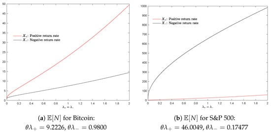
Figure 1. Empirical behavior of $\mathbb{E}\left[N\right]$ for Bitcoin and S&P 500 index.

• For negative Bitcoin returns (black curve) and positive S&P 500 returns (red curve), $\mathbb{E}\left[N\right]$ grows slowly.
• However, for negative S&P 500 returns (also shown in black), $\mathbb{E}\left[N\right]$ increases exponentially, leading to a prohibitively large number of trials.

The rapid increase in the expected number of trials results in a poor acceptance rate for large values of $\lambda$ or for small values of $\beta$. The expected number of trials ($\mathbb{E}\left[N\right]$) is referred to as the “expected complexity” in the literature [12,14,16,43]. The high expected complexity results in a high rejection rate, rendering the SSR algorithm inefficient and limiting its practical application.

The empirical values of $\mathbb{E}\left[N\right]$ for financial assets, including the S&P 500 index, SPY ETF, Bitcoin, and Ethereum, were computed and summarized in Table 3.

Table 3. Transformed parameters and GTS parameters.

		GTS Distribution Parameters				Transformed Parameters
Financial Assets	Variable	$\mathit{\mu }$	$\mathit{\beta }$	$\mathit{\alpha }$	$\mathit{\lambda }$	$\mathit{\theta }$	$\mathit{\theta }\mathit{\lambda }$	$\mathbb{E}\left[\mathit{N}\right]$
S&P 500 index	$X_{+}$	−0.24941	0.32862	0.79243	1.27974	35.9485	46.0049	33.7557
	$X_{-}$		0.08864	0.54225	0.93713	$1.4\times {10}^9$	$1.3\times {10}^9$	629.582
SPY ETF	$X_{+}$	−0.26064	0.34088	0.78776	1.28856	29.2566	37.6987	31.3803
	$X_{-}$		0.02221	0.59711	1.01435	$4.1\times {10}^{64}$	$4.2\times {10}^{64}$	$6.8\times {10}^{11}$
Bitcoin	$X_{+}$	−0.12157	0.31555	0.74771	0.24653	37.4095	9.2226	7.5071
	$X_{-}$		0.40646	0.54457	0.17477	5.6072	0.9800	2.6961
Ethereum	$X_{+}$	−0.48538	0.39044	0.95825	0.16671	26.6355	4.4405	5.9876
	$X_{-}$		0.40448	0.80048	0.17079	14.7212	2.5142	4.2715

The transformed parameters $\theta$ and $\theta \lambda$ exhibit significantly larger values for the S&P 500 index and SPY ETF, with the expected complexities of $629.582$ and 6.8 $\times {10}^{11}$, respectively. The high values make the SSR algorithm not applicable to the financial assets: S&P 500 index and SPY ETF.

Algorithm 1 outlines the SSR sampling approach [16,43,44], commonly used for sampling from exponentially tilted stable distributions, also known as generalized gamma distributions [41].

Algorithm 1 Standard Stable Rejection (SSR) sampling [14].

1: loop 2:      Draw $X\sim S_{\beta }(1,\delta ,0)$              ▹ via Chambers–Mallows–Stuck (CMS) method (see (16)) 3:      Draw $U\sim \mathrm{Uniform}(0,1)$                                                                 ▹ U and X independent 4:      if $U<e^{-\lambda X}$ then 5:           return $X_{\lambda }=X$                                       ▹ Accept: exponential tilting of the stable law 6:      else 7:           Reject X, restart Stage 1 8:      end if 9: end loop

To evaluate the performance of Algorithm 1, we generated a sample of 80,000 data points to mimic the two financial assets: Bitcoin and Ethereum. As shown in Figure 2b and Figure 3b, the Q-Q plots maintain smooth linear patterns, confirming the alignment of the empirical and theoretical distributions.

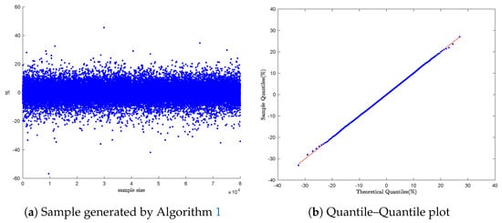
Figure 2. Bitcoin daily return simulation: Q-Q Plot with Algorithm 1.

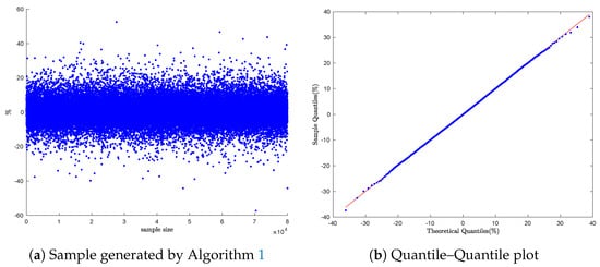
Figure 3. Ethereum daily return simulation: Q-Q Plot with Algorithm 1.

Remark 9.

The theoretical quantiles (represented by the red line in the Q-Q plot) and the observed quantiles were computed by the Enhanced Fast Fractional Fourier Transform (FRFT) scheme. The Enhanced Fast FRFT scheme improves the accuracy of the one-dimensional Fast FRFT by leveraging closed Newton–Cotes quadrature rules [45,46]. For more details on the methodology and its applications, refer to [21,47,48].

The Standard Stable Rejection (SSR) method is theoretically appealing but becomes impractical for large tempering parameters ($\lambda \to +\infty$) or small stability index parameter ($\beta \to 0$) due to unbounded computational complexity. While useful for small-scale simulations with moderate parameters, its limitations make it unsuitable for financial modeling, where extreme parameter values are common.

The Fast Rejection Algorithm [16,43] significantly reduces the expected complexity of SSR sampling down to logarithmic expected complexity. However, like SSR, its expected runtime is still unbounded, meaning performance can degrade for extreme parameter values ($\beta$). By contrast, both the Double Rejection and Two-Dimensional Single Rejection algorithms ensure a bounded expected complexity for all $\beta \in (0,1)$ and $\lambda >0$.

5.2. Double Rejection Method

The joint density function $h(x,u)$ in (30) serves as the target distribution for sampling the marginal random variable $X_{\lambda }$.

The marginal density of $X_{\lambda }$ is given by the integral in (32), which does not have a closed-form expression:

$$f\left(x\right)={\int }_0^{\pi }h(x,u)du={\int }_0^{\pi }{\displaystyle \frac{e^{{\lambda }^{\beta }}B{\left(u\right)}^{\frac{1}{1-\beta }}}{\pi }}{e}^{-\lambda x^{-{\displaystyle \frac{1-\beta }{\beta }}}-B{\left(u\right)}^{{\displaystyle \frac{1}{1-\beta }}}x}du.$$

(32)

Similarly, the marginal density function of U, given by (33), lacks a closed-form solution:

$$h\left(u\right)={\int }_0^{\infty }h(x,u)dx={\displaystyle \frac{e^{{\lambda }^{\lambda }}B{\left(u\right)}^{\frac{1}{1-\beta }}}{\pi }}{\int }_0^{\infty }{e}^{-\lambda x^{-{\displaystyle \frac{1-\beta }{\beta }}}-B{\left(u\right)}^{{\displaystyle \frac{1}{1-\beta }}}x}dx.$$

(33)

To generate samples of $X_{\lambda }$, one approach is to first sample U and then generate $X_{\lambda }$ from the conditional density $h(x\mid U)$. However, the lack of a closed-form expression for $h\left(u\right)$ complicates this process. The Double Rejection method addresses this challenge by selecting an appropriate bivariate density function $g(x,u)$ and a univariate density function $k\left(u\right)$ such that

$$\begin{array}{c}\hfill h(x,u)\le g(x,u),g^{*}\left(u\right)={\int }_0^{\infty }g(x,u)dx,g^{*}\left(u\right)\le k\left(u\right).\end{array}$$

(34)

These functions are chosen to facilitate efficient sampling of $X_{\lambda }$. The first-level rejection method is used to sample U from the marginal density $g^{*}\left(u\right)$, while the second-level rejection method generates the bivariate random variable $(X,U)$ with density function $h(y,u)$. The Double Rejection method, introduced by [12], uses the following bivariate and univariate density functions.

$$g(y,u)=\left\{\begin{array}{cc}{\displaystyle \frac{A\left(u\right)e^{{\lambda }^{\lambda }}}{\pi }}{e}^{-{\displaystyle \frac{A\left(u\right)}{1-\beta }}m-{\displaystyle \frac{1}{2}}{\left({\displaystyle \frac{y-m)}{\gamma }}\right)}^2}\hfill & y\le m\hfill \\ {\displaystyle \frac{A\left(u\right)e^{{\lambda }^{\lambda }}}{\pi }}{e}^{-{\displaystyle \frac{A\left(u\right)}{1-\beta }}m}\hfill & m\le y\le m+\delta \hfill \\ {\displaystyle \frac{A\left(u\right)e^{{\lambda }^{\lambda }}}{\pi }}{e}^{-{\displaystyle \frac{A\left(u\right)}{1-\beta }}m-(y-m-\delta )\lambda }\hfill & m+\delta \le y\hfill \end{array}\right. k\left(u\right)=\left\{\begin{array}{cc}{w}_1{f}_1\left(u\right)+w_2{f}_2\left(u\right)\hfill & \gamma \ge 1\hfill \\ w_3{f}_3\left(u\right)+w_2{f}_2\left(u\right)\hfill & \gamma \le 1,\hfill \end{array}\right.$$

where the parameters and the weight coefficients are defined as follows:

• $A\left(u\right)=B{\left(u\right)}^{{\displaystyle \frac{1}{1-\beta }}}$; $m={\left({\displaystyle \frac{(1-\beta )\lambda }{\beta A\left(u\right)}}\right)}^{\beta }$; $\gamma =\beta (1-\beta ){\lambda }^{\beta }$; $\delta =\sqrt{{\displaystyle \frac{m\beta }{A\left(u\right)}}}$.
• $w_1=\xi \sqrt{{\displaystyle \frac{\pi }{2\sigma }}}$, $f_1\left(u\right)$ is normal density with $\mu =0$ and $\sigma =\sqrt{2\pi \gamma }$.
• $w_2=2\psi \sqrt{\pi }$, $f_2\left(u\right)$ is beta density with $a=1$ and $b={\displaystyle \frac{1}{2}}$.
• $w_3=\xi \pi$, $f_3\left(u\right)$ is uniform distribution over $(0,\pi )$.

The following theorem from [12] establishes that the expected complexity of the Double Rejection method is uniformly bounded for all values of $\beta \in (0,1)$ and $\lambda >0$.

Theorem 6.

Let $R(\beta ,\lambda )$ be the expected number of iterations required to generate a random variable $X_{\lambda }$ using the Double Rejection method. Then,

$$\begin{array}{c}\hfill \underset{\begin{array}{c}\beta \in (0,1)\\ \lambda >0\end{array}}{Sup}R(\beta ,\lambda )\le 8.11328125.\end{array}$$

(35)

The proof of Theorem 6 can be found in [12].

The GTS parameter estimates presented in Table 1 and Table 2 were used to simulate the daily returns of each financial asset. For each asset, empirical quantiles were computed from the observed daily return samples. The Q-Q plots shown in Figure 4a,b and Figure 5a,b compare these sample quantiles with the theoretical quantiles derived from the General Tempered Stable (GTS) distribution. The plots display a smooth non-linear pattern in the central region and noticeable discrepancies in the tails.

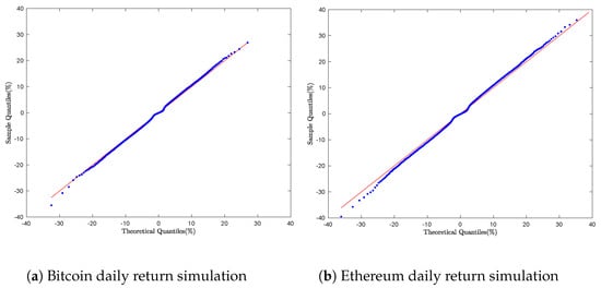
Figure 4. Cryptocurrency daily return simulation: Q-Q Plot with Algorithm 2.

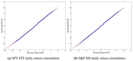
Figure 5. Equity daily return simulation: Q-Q Plot with Algorithm 2.

The graphical results suggest that the empirical return distributions exhibit heavier tails than those predicted by the GTS model, indicating limitations in the Double Rejection method’s ability to accurately capture the GTS model’s extreme values.

Despite its theoretically established complexity bounds, the Double Rejection technique proves inadequate for accurate GTS simulations, as it fails to capture the heavy-tailed characteristics of the distribution.

Algorithm 2 Double Rejection sampling.

Require:  Marginal density $g^{*}\left(u\right)$, proposal density $k\left(u\right)$, joint density $h(x,u)$, and proposal $g(x\mid u)$. Ensure:  Sample $X\sim h(x,u)$ marginalized over u.   1: Input: Parameters $\alpha ,\beta ,\lambda$   2: Initialize: $\mathrm{\Gamma }\leftarrow 0$, $\mathrm{sum}\leftarrow 0$, $\mathrm{y}\leftarrow 1$ set threshold $\epsilon ={10}^{-5}$   3: loop   4:       Draw $U\sim k\left(u\right)$                          ▹ Stage 1: sample U   5:       Draw $W\sim \mathrm{Unif}(0,1)$                     ▹U and W independent   6:       if ${\displaystyle W<\frac{g^{*}\left(U\right)}{k\left(U\right)}}$ then   7:            Accept U   8:            Set ${\displaystyle V\leftarrow W·\frac{k\left(U\right)}{g^{*}\left(U\right)}}$   9:       else 10:            Reject U, retry Stage 1 11:       end if 12:       Draw $X\sim g(x\mid U)$                        ▹ Stage 2: sample X 13:       if ${\displaystyle V<\frac{h(X,U)}{g(X,U)}}$ then 14:            return X 15:       else 16:            Reject $(U,X)$, restart Stage 1 17:       end if 18:        Return $X_{\lambda }=X^{-{\displaystyle \frac{1-\beta }{\beta }}}$. 19: end loop

5.3. Two-Dimensional Single Rejection Method

The joint density function $f(x,u)$ in (28) serves as the target distribution for sampling the bivariate variable $(X,U)$. The Two-Dimensional Single Rejection method [14] uses a proposal bivariate density function $g(x,u)$, along with a constant $C(\beta ,\lambda )$ such that

$$\begin{array}{c}\hfill f(x,u)\le C(\beta ,\lambda )g(x,u).\end{array}$$

(36)

This method generates samples $(X,U)$ from the target distribution $f(x,u)$ by first generating candidates from the proposal density function $g(x,u)$ and then rejecting a subset of these candidates based on the relationship in (36).

Algorithm 3 outlines the Two-Dimensional Single Rejection sampling approach.

Algorithm 3 Two-Dimensional Single Rejection sampling [14].

1: Input: Parameters $\alpha ,\beta ,\lambda$   2: Set $C(\beta ,\lambda )={sup}_{x,u}\left\{{\displaystyle \frac{f(x,u)}{g(x,u)}}\right\}$   3: loop                      ▹ Envelope constant ensuring $f\le Cg$   4:       Sample $(X,U)\sim g(x,u)$        ▹ Draw a sample from the proposal distribution   5:       Draw $W\sim \mathrm{Uniform}(0,1)$                    ▹ Independent of $(X,U)$   6:       if $W<{\displaystyle \frac{f(X,U)}{C(\beta ,\lambda )g(X,U)}}$ then   7:             Accept $(X,U)$              ▹ Accepted proposal under joint envelope   8:       else   9:             Reject $(X,U)$, restart from Step 2 10:       end if 11:       return $X_{\lambda }=K\left(X\right)$             ▹$K\left(X\right)={\displaystyle \frac{X}{\lambda }}$ or $K\left(X\right)=B^{{\displaystyle \frac{1}{\beta }}}\left(u\right)X^{-{\displaystyle \frac{1-\beta }{\beta }}}$ 12: end loop

For a given $(\beta ,\lambda )$, the two types of proposal bivariate density function, denoted as $g(x,u)$, are considered by the Two-Dimensional Single Rejection method:

• First proposal bivariate density function: A product of the gamma density function and the uniform density function. This approach has expected complexities denoted by $C_1(\beta ,\lambda )$ and $C_2(\beta ,\lambda )$, yielding the target random variable $X_{\lambda }={\displaystyle \frac{X}{\lambda }}$.
• Second proposal bivariate density function: A product of a gamma density function and a normal density function. The expected complexities in this case are $C_3(\beta ,\lambda )$ and $C_4(\beta ,\lambda )$, resulting in the target random variable $X_{\lambda }=B^{{\displaystyle \frac{1}{\beta }}}\left(u\right)X^{-{\displaystyle \frac{1-\beta }{\beta }}}$.

Table 4 provides additional details on the implementation of the Two-Dimensional Single Rejection algorithm (Algorithm 3).

Table 4. Describtion of the proposal bivariate density functions [14].

$\mathit{g}(\mathit{x},\mathit{u})$	(X, U)	$\mathit{C}(\mathit{\beta },\mathit{\lambda })$	${\mathit{X}}_{\mathit{\lambda }}$
Gamma and Unform bivariate	$X\sim \mathrm{\Gamma }(\beta {\lambda }^{\beta },1),U\sim U(0,\pi )$	$C_1(\beta ,\lambda )$	${\displaystyle \frac{X}{\lambda }}$
Gamma and Unform bivariate	$X\sim \mathrm{\Gamma }((1-\beta ){\lambda }^{\beta }+1,1),U\sim U(0,\pi )$	$C_2(\beta ,\lambda )$	${\displaystyle \frac{X}{\lambda }}$
Gamma and truncated normal bivariate	$X\sim \mathrm{\Gamma }(\beta {\lambda }^{\beta },1),U\sim N(0,{\sigma }^2,lb=0,ub=\pi )$	$C_3(\beta ,\lambda )$	$B^{{\displaystyle \frac{1}{\beta }}}\left(u\right)X^{-{\displaystyle \frac{1-\beta }{\beta }}}$
Gamma and truncated normal bivariate	$X\sim \mathrm{\Gamma }((1-\beta ){\lambda }^{\beta }+1,1),U\sim N(0,{\sigma }^2,{lb}^1=0,ub=\pi ))$	$C_4(\beta ,\lambda )$	$B^{{\displaystyle \frac{1}{\beta }}}\left(u\right)X^{-{\displaystyle \frac{1-\beta }{\beta }}}$

¹ ${\sigma }^2={\displaystyle \frac{1}{\beta (1-\beta ){\lambda }^{\beta }}}$    lb(ub) stands for lower bound (upper bound).

The expected complexities $C_1(\beta ,\lambda )$, $C_2(\beta ,\lambda )$, $C_3(\beta ,\lambda )$, and $C_4(\beta ,\lambda )$ are further examined using empirical values based on parameters derived from financial assets, including the S&P 500 index, SPY ETF, Bitcoin, and Ethereum. As shown in Table 5, $C_1(\beta ,\lambda )$ and $C_3(\beta ,\lambda )$ demonstrate greater stability and are less affected by large parameter values, such as $\theta {\lambda }_{-}=1.3\times {10}^9$ for the S&P 500 index and $\theta {\lambda }_{-}=4.2\times {10}^{64}$ for the SPY ETF.

Table 5. Expected complexity empirical values.

		Parameters		Expected Complexities
Financial Assets	Variable	$\mathit{\beta }$	$\mathit{\theta }\mathit{\lambda }$	${\mathit{C}}_{\mathbf{1}}(\mathit{\beta },\mathit{\theta }\mathit{\lambda })$	${\mathit{C}}_{\mathbf{2}}(\mathit{\beta },\mathit{\theta }\mathit{\lambda })$	${\mathit{C}}_{\mathbf{3}}(\mathit{\beta },\mathit{\theta }\mathit{\lambda })$	${\mathit{C}}_{\mathbf{4}}(\mathit{\beta },\mathit{\theta }\mathit{\lambda })$	$\mathit{C}(\mathit{\beta },\mathit{\theta }\mathit{\lambda })$
S&P 500 index	$X_{+}$	0.32862	46.0049	3.4868	3.9905	1.5787	1.8067	1.5787
	$X_{-}$	0.08864	$1.3\times {10}^9$	2.3536	6.1617	1.3013	3.4068	1.3013
SPY ETF	$X_{+}$	0.34088	37.6987	3.5339	3.9181	1.6022	1.7764	1.6022
	$X_{-}$	0.02221	$4.2\times {10}^{64}$	2.2609	12.979	1.1725	6.7309	1.1725
Bitcoin	$X_{+}$	0.31555	9.2226	3.0452	3.1247	1.8412	1.8893	1.8412
	$X_{-}$	0.40646	0.9800	3.4102	2.1960	2.7813	1.7910	1.7910
Ethereum	$X_{+}$	0.39044	4.4405	3.3652	2.8209	2.0570	1.7243	1.7243
	$X_{-}$	0.40448	2.5142	3.3829	2.5581	2.2820	1.7256	1.7256

The overall complexity ($C(\beta ,\lambda )$) of the Two-Dimensional Single Rejection is defined as follows:

$$C(\beta ,\lambda )=\underset{\begin{array}{c}1\le k\le 4\end{array}}{Min}\left\{C_k(\beta ,\lambda ):(\beta ,\lambda )\in (0,1)x(0,\infty )\right\}.$$

(37)

Theorem 7.

The complexity $C(\beta ,\lambda )$ in Equation (37) for Algorithm 3 is uniformly bounded, satisfying the following relationship:

$$\underset{\begin{array}{c}\beta \in (0,1)\\ \lambda >0\end{array}}{Sup}C(\beta ,\lambda )\le 4.2154$$

(38)

Consult [14] for the proof of Theorem 7.

As shown in Table 5, the overall complexity ($C(\beta ,\lambda )$) remains more stable and below the upper bound of $4.2154$. However, the individual expected complexities $C_3(\beta ,\lambda )$ and $C_4(\beta ,\lambda )$ do not satisfy the relationship in (38) for S&P 500 index and SPY ETF data.

To evaluate the performance of Algorithm 3, we generated a sample of 8000 daily returns for each financial asset. The empirical distributions were compared against the theoretical distributions using Q-Q plots. The results of this distributional analysis are presented in Figure 6a,b and Figure 7a,b.

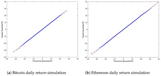
Figure 6. Cryptocurrency daily return simulation: Q-Q Plot with Algorithm 3.

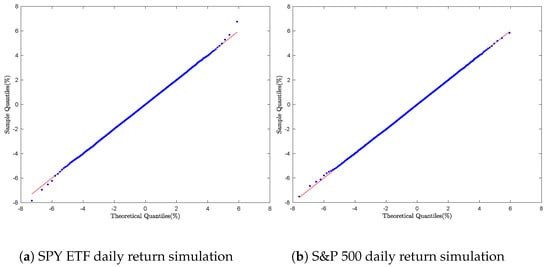
Figure 7. Equity daily return simulation: Q-Q Plot with Algorithm 3.

As shown in each plot, the Q-Q plots display a smooth linear pattern, indicating a strong alignment between the empirical distributions and the theoretical GTS distribution.

The Two-Dimensional Single Rejection method outperforms other rejection-based approaches by offering greater stability across parameter ranges. It effectively captures both the central and tail behavior of the GTS distribution, making it more accurate and reliable for simulations.

Remark 10.

In a Q-Q plot, the quantiles of the observed distribution are plotted against those of the theoretical distribution. When the two distributions are similar, their quantiles will be nearly equal, and the points will closely follow the line $X=Y$. Any deviation from this line reveals differences between the distributions. The following scenarios, commonly observed in the literature [49,50,51,52,53], are worth noting:

1. 

Q-Q Plots and Skewed Distributions: A left-skewed distribution typically results in a concave downward Q-Q plot, while a right-skewed distribution shows a U-shaped or “humped” pattern. A symmetric distribution, on the other hand, will usually produce a symmetric and linear Q-Q plot around the center of the data.

2. 

Q-Q Plots and Short-Tailed Distributions: Short-tailed distributions may exhibit an S-shaped curve in the Q-Q plot. More specifically, the deviation from the straight line appears in the opposite direction at the tails compared to long-tailed distributions (above the line in the lower tail and below the line in the upper tail).

3. 

Q-Q Plots and Long-Tailed Distributions: Long-tailed distributions typically show deviations from the straight line at both ends of the Q-Q plot, with the lower tail curving downward and the upper tail curving upward.

4. 

S-shaped Curves in Q-Q Plots: An S-shaped curve can indicate several potential issues, such as longer or shorter tails than the theoretical distribution, or systematic differences between the distributions being compared.

6. Series Representation Methods for Simulating GTS Lévy Processes

We develop a simulation framework for Generalized Tempered Stable (GTS) Lévy processes based on almost surely convergent series representations. These representations, originally proposed by Rosiński [19] and later adapted to Tempered Stable distributions in [54], offer theoretically sound methods for generating sample paths of Lévy processes. In this context, we focus on two principal constructions: the inverse Lévy measure series representation and the Shot Noise series representation. These representations will serve as the basis for simulating GTS random variates.

Let $X\left(t\right)$, $t\in [0, 1]$ be a d-dimensional Lévy process with stationary, independent increments, stochastically continuous, and starting at zero. Its characteristic function is

$$\mathbb{E}\left[e^{i\xi X\left(t\right)}\right]=e^{t\varphi \left(\xi \right)},$$

(39)

where

$$\varphi \left(\xi \right)=i\xi \mu +{\int }_{\mathbb{R}\backslash \left\{0\right\}}\left(e^{i\xi y}-1-i\xi y\mathbb{I}\left(\right|y|\le 1)\right)\nu \left(dy\right),$$

(40)

with

• $\varphi \left(\xi \right)$: characteristic exponent;
• $\mu \in {\mathbb{R}}^d$: drift vector;
• $\nu$: Lévy measure, defining the intensity and distribution of jumps in the process, and satisfying $\int \left(\right|y{|}^2\wedge 1)\nu \left(dy\right)<\infty$;
• $(\mu ,0,\nu )$: characteristic triplet of X.

According to the Lévy–Itô decomposition theorem [19,55], $X\left(t\right)$ admits the following decomposition:

$$X\left(t\right)=t\mu +{\int }_{\left|x\right|\le 1}x[N([0,t],dx)-t\nu \left(dx\right)]+{\int }_{\left|x\right|>1}xN([0,t],dx),$$

(41)

where N is a Poisson random measure on $(0,\infty )\times ({\mathbb{R}}^d\backslash \left\{0\right\})$. Equivalently,

$$N=\sum _{i=1}^{\infty }{\delta }_{(U_i,J_i)},$$

(42)

with $U_i\sim \mathrm{Unif}[0,1]$ i.i.d. and $J_i\in {\mathbb{R}}^d$ as the associated jump sizes, independent from the $U_i$. For further details, please refer to [19,56,57].

For $n\in \mathbb{N}$, we define

$$\begin{array}{c}\hfill X_n\left(t\right)=t\mu +{\int }_{{\displaystyle \frac{1}{n}}\le \left|x\right|\le 1}x\left[\left(N\right([0,t],dx)-tV(dx)\right]+{\int }_{\left|X\right|\ge 1}xN([0,t],dx.\end{array}$$

(43)

By replacing (42) in (43), we have

$$\begin{array}{c}\hfill X_n\left(t\right)=t\mu -t{b}_n+\sum _{i\in k_n}{J}_{i}1(U_i\le t),\end{array}$$

(44)

where

$$\begin{array}{c}\hfill k_n=\left\{1\le i:{\displaystyle \frac{1}{n}}\le \left|J_i\right|\right\},b_n={\int }_{{\displaystyle \frac{1}{n}}\le \left|x\right|\le 1}xV\left(dx\right).\end{array}$$

As $n\to \infty$, this converges almost surely to

$$\begin{array}{c}\hfill X\left(t\right)=\underset{n=\infty }{lim}{X}_n\left(t\right)=t\mu +\sum _{i=1}^{\infty }\left[J_{i}1(U_i\le t)-t{c}_i\right],c_i=b_i-b_{i-1},\end{array}$$

(45)

and we have

$$\begin{array}{c}\hfill X\left(t\right)=t\mu +\sum _{i=1}^{\infty }\left[J_{i}1(U_i\le t)-t{c}_i\right].\end{array}$$

(46)

In the special case of GTS distribution where $d=1$, $X\sim GTS({\beta }_{+},{\beta }_{-},{\alpha }_{+},{\alpha }_{-},{\lambda }_{+},{\lambda }_{-})$ and the characteristic exponent becomes

$$\varphi \left(\xi \right)=i\xi \mu +{\int }_{\mathbb{R}\backslash \left\{0\right\}}\left(e^{i\xi y}-1)\right)\nu \left(dy\right).$$

(47)

The Lévy–Itô decomposition Equation (41) becomes Equation (48):

$$X\left(t\right)=t\mu +{\int }_{\left|x\right|>0}xN([0,t],dx)=t\mu +{\int }_{x>0}xN([0,t],dx)+{\int }_{x<0}xN([0,t],dx).$$

(48)

Following the procedure developed previously (from Equation (41) to Equation (45)), Equation (46) becomes Equation (49):

$$X\left(t\right)=t\mu +\sum _{i=1}^{\infty }\left[J_i^{+}1(U_i^{+}\le t)\right]-\sum _{i=1}^{\infty }\left[J_i^{-}1(U_i^{-}\le t)\right],$$

(49)

with $U_i^{+}\sim \mathrm{Unif}[0,1]$ i.i.d. and $J_i^{+}\in {\mathbb{R}}^{+}$ as the associated jump sizes, independent from the $U_i^{+}$. Similarly on the left side, $U_i^{-}\sim \mathrm{Unif}[0,1]$ i.i.d. and $J_i^{-}\in {\mathbb{R}}^{+}$ are the associated jump sizes, independent from the $U_i^{-}$.

6.1. Sampling GTS Distribution via the Inverse Lévy Measure Series Representation

Let $X_{+}\sim TS(\beta ,\alpha ,\lambda )$, where $TS(\beta ,\alpha ,\lambda )$ denotes a Tempered Stable distribution. The Lévy measure of $X_{+}$ is concentrated on $(0,\infty )$ and the Tail Integral function is defined as follows:

$$\begin{array}{c}\hfill W^{+}\left(y\right)=\alpha {\int }_y^{\infty }{x}^{-1-\beta }{e}^{-\lambda x}dx.\end{array}$$

(50)

Using integration by parts, Equation(50) becomes

$$\begin{array}{c}\hfill W^{+}\left(y\right)={\displaystyle \frac{\alpha }{\beta }}{y}^{-\beta }{e}^{-\lambda y}-{\displaystyle \frac{\alpha {\lambda }^{\beta }}{\beta }}\mathrm{\Gamma }(1-\beta ,\lambda y),\end{array}$$

(51)

where $\mathrm{\Gamma }(\alpha ,y)={\int }_y^{\infty }{x}^{\alpha -1}{e}^{-x}dx$ is the upper incomplete gamma function.

The inverse of the Tail Integral function ${W^{+}}^{\leftarrow }$ is defined as follows:

$$\begin{array}{c}\hfill {W^{+}}^{\leftarrow }\left(\mathrm{\Gamma }\right)=inf\{y>0:W\left(y\right)<\mathrm{\Gamma }\}.\end{array}$$

The series representation generated by the inverse Lévy measure method of $X_{+}$ has the following expression:

$$\begin{array}{cc}\hfill X_{+}\left(t\right)& =\sum _{i=1}^{\infty }\left[{W^{+}}^{\leftarrow }\left({\mathrm{\Gamma }}_i^{+}\right)1(U_i^{+}\le t)\right].t\in [0,1],\hfill \end{array}$$

(52)

$$\begin{array}{cc}\hfill X_{+}\left(1\right)& =\sum _{i=1}^{\infty }{W^{+}}^{\leftarrow }\left({\mathrm{\Gamma }}_i^{+}\right),\hfill \end{array}$$

(53)

where

• ${\mathrm{\Gamma }}_j-{\mathrm{\Gamma }}_{j-1}$, $E_j$ are i.i.d. exponential random variables with mean 1, and we set ${\mathrm{\Gamma }}_0=0$;
• $\left\{U_j\right\}$ are i.i.d. uniform random variables on $[0, 1]$;
• All the random elements $\left\{U_j\right\}$, $\left\{{\mathrm{\Gamma }}_j\right\}$ are mutually independent.

Algorithm 4 outlines the simulation of $X_{+}$ on [0, 1] using the series representation generated by the inverse Lévy measure method.

Algorithm 4 Series representation using the inverse Lévy measure method.

1: Input: Parameters $\alpha ,\beta ,\lambda$ and time horizon $t=1$   2: loop   3:       Initialize: $\mathrm{\Gamma }\leftarrow 0$, $\mathrm{sum}\leftarrow 0$, $\mathrm{y}\leftarrow 1$ set threshold $\epsilon ={10}^{-5}$   4:       while $y>\epsilon$ do   5:             Draw $v_1\sim \mathrm{Unif}(0,1)$   6:             $\mathrm{\Gamma }\leftarrow \mathrm{\Gamma }-ln{v}_1$     (next Poisson arrival time)   7:             Solve $\mathrm{\Gamma }=W^{+}\left(y\right)$ numerically for $y=W^{-1}\left(\mathrm{\Gamma }\right)$   8:             Draw $u\sim \mathrm{Unif}(0,1)$   9:             if $u<t$ then 10:                   $\mathrm{sum}\leftarrow \mathrm{sum}+y$ 11:             end if 12:       end while 13:       return $\mathrm{sum}$ 14: end loop

Daily return samples for Bitcoin, Ethereum, the S&P 500, and the SPY ETF were generated using the series representation in Equation (53). For each asset, empirical quantiles were computed and compared to theoretical quantiles through Q-Q plots.

As illustrated in Figure 8 and Figure 9, Figure 8a,b and Figure 9a,b exhibit smooth linearity patterns, indicating a strong agreement between the empirical and theoretical distributions for each asset.

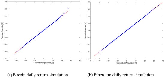
Figure 8. Cryptocurrency daily return simulation: Q-Q Plot with Algorithm 4.

Figure 9. Equity daily return simulation: Q-Q Plot with Algorithm 4.

The inverse Lévy measure method achieves exact simulation by inverting $W^{+}\left(y\right)$, offering a precise series representation, strong empirical performance, and better tail-fitting than rejection-based techniques. However, because it relies on iterative numerical inversion, it is computationally intensive, making it practical only for moderate-scale simulations rather than large-scale applications.

6.2. Sampling GTS Distribution via the Shot Noise Series Representation

The inverse of the tail of the Lévy measure for a Tempered Stable distribution lacks a closed-form expression, as shown in Equation (50). As a result, the inverse Lévy measure method becomes practically intractable. To address this difficulty, Rosiński [5,18,19,54] proposes a series representation based on the generalized Shot Noise framework, which is more revealing about the structure of the Tempered Stable distribution:

Theorem 8

(Theorem 5.1 [18]). Let $X\left(t\right)$, $t\in [0, 1]$, be a tempered stable Lévy process in ${\mathbb{R}}^d$ with $\mathcal{L}\left(X\right(1\left)\right)\sim \mathrm{TS}(\alpha ,\nu ;0)$; if $\beta \in (0, 1)$, or ν is symmetric and $\beta \in (0, 2)$, then

$$\begin{array}{c}\hfill X\left(t\right)\stackrel{d}{=}\sum _{j=1}^{\infty }{V}_j\left({\displaystyle \frac{m\left(\nu \right)}{\parallel V_j\parallel }}{\left(\beta {\mathrm{\Gamma }}_j\right)}^{-{\displaystyle \frac{1}{\beta }}}\wedge E_j{U}_j^{{\displaystyle \frac{1}{\beta }}}\right){\mathbf{1}}_{\{T_j\le 1\}}\left(t\right),t\in [0, 1],\end{array}$$

(54)

where the equality holds in the sense of finite-dimensional distributions, and the infinite series converges almost surely, uniformly in $t\in [0, 1]$. Here,

• $\left\{T_j\right\}$, $\left\{U_j\right\}$ are i.i.d. uniform random variables on $[0, 1]$.
• ${\mathrm{\Gamma }}_j-{\mathrm{\Gamma }}_{j-1}$, $E_j$ are i.i.d. exponential random variables with mean 1, and we set ${\mathrm{\Gamma }}_0=0$.
• $\left\{V_j\right\}$ are i.i.d. random vectors in ${\mathbb{R}}^d$ with common distribution ${\nu }_1$, defined via the Lévy measure ν by

  $$\begin{array}{c}\hfill {\nu }_1\left(dx\right)={\displaystyle \frac{1}{m{\left(\nu \right)}^{\beta }}}{\parallel x\parallel }^{\beta }\nu \left(dx\right),m\left(\nu \right)={\left({\int }_{\{\parallel x\parallel >0\}}{\parallel x\parallel }^{\beta }\nu \left(dx\right)\right)}^{{\displaystyle \frac{1}{\beta }}}.\end{array}$$

  (55)
• All the random elements $\left\{T_j\right\}$, $\left\{U_j\right\}$, $\left\{{\mathrm{\Gamma }}_j\right\}$, $\left\{E_j\right\}$, and $\left\{V_j\right\}$ are mutually independent.

Refer to [5] for the proof of Theorem 8.

For the one-sided case, let $X_{+}\sim TS(\beta ,\alpha ,\lambda )$ denote a Tempered Stable distribution. The Lévy measure of $X_{+}$ is concentrated on $(0,\infty )$ with dimension $d=1$. Using the notation from [5], we have $X_{+}\sim T{S}_{\beta }^0(\alpha {\lambda }^{\beta }{\delta }_{{\lambda }^{-1}},0)$ for a time horizon $t=1$:

$$\begin{array}{c}\hfill \nu =\alpha {\lambda }^{\beta }{\delta }_{{\lambda }^{-1}},m\left(\nu \right)={\left({\int }_{\{\parallel x\parallel >0\}}{\parallel x\parallel }^{-\beta }\nu \left(dx\right)\right)}^{{\displaystyle \frac{1}{\beta }}}={\alpha }^{{\displaystyle \frac{1}{\beta }}},{\nu }_1\left(dx\right)={\lambda }^{\beta }{\parallel x\parallel }^{\beta }{\delta }_{{\lambda }^{-1}}\left(dx\right).\end{array}$$

The common distribution ${\nu }_1$ is related to the Dirac measure ${\delta }_{{\lambda }^{-1}}$, implying that $V_j={\lambda }^{-1}$ is deterministic.

The sampling of daily returns for Bitcoin, Ethereum, the S&P 500, and the SPY ETF was performed using Equation (57), which corresponds to a version of Equation (56) with time horizon $t=1$:

$$\begin{array}{cc}\hfill X_{+}\left(t\right)& =\sum _{j=1}^{\infty }\left({\left({\displaystyle \frac{\alpha }{\beta {\mathrm{\Gamma }}_j}}\right)}^{1/\beta }\wedge e_j{u}_j^{{\displaystyle \frac{1}{\beta }}}{\lambda }^{-1}\right){\mathbf{1}}_{\{T_j\le 1\}}\left(t\right),t\in [0,1]\hfill \end{array}$$

(56)

$$\begin{array}{cc}\hfill X_{+}\left(1\right)& =\sum _{j=1}^{\infty }\left({\left({\displaystyle \frac{\alpha }{\beta {\mathrm{\Gamma }}_j}}\right)}^{1/\beta }\wedge e_j{u}_j^{{\displaystyle \frac{1}{\beta }}}{\lambda }^{-1}\right).\hfill \end{array}$$

(57)

Algorithm 5 describes how to simulate $X_{+}\left(1\right)$ using the Shot Noise series representation.

Algorithm 5 Shot Noise representation for $X_{+}\left(1\right)$.

1: Input: Parameters $\alpha ,\beta ,\lambda$ and time horizon $t=1$   2: loop   3:       Initialize: $\mathrm{\Gamma }\leftarrow 0$, $\mathrm{sum}\leftarrow 0$; set threshold $\epsilon ={10}^{-5}$   4:       while $w>\epsilon$ do   5:             Draw $v\sim U(0,1)$; update $\mathrm{\Gamma }\leftarrow -lnv+\mathrm{\Gamma }$   6:             Compute $w_1\leftarrow {\left(\alpha /\left(\beta \mathrm{\Gamma }\right)\right)}^{1/\beta }$   7:             Draw $v\sim U(0,1)$, $u\sim U(0,1)$; set $E=-lnv$   8:             Compute $w_2\leftarrow E{u}^{1/\beta }{\lambda }^{-1}$; let $w\leftarrow min(w_1,w_2)$   9:             if $T_j=u<t$ then 10:                   $\mathrm{sum}\leftarrow \mathrm{sum}+w$ 11:             end if 12:       end while 13:       return $\mathrm{sum}$ 14: end loop

For each financial asset, empirical quantiles were computed and compared to theoretical quantiles through Q-Q plots, As illustrated in Figure 10 and Figure 11.

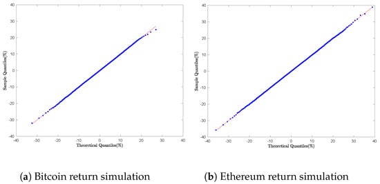
Figure 10. Cryptocurrency daily return simulation: Q-Q Plot with Algorithm 5.

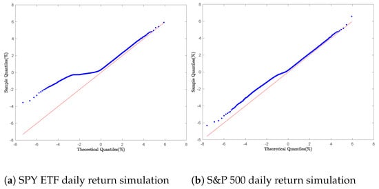
Figure 11. Equity daily return simulation: Q-Q Plot with Algorithm 5.

Figure 10a,b exhibit smooth linear patterns, indicating strong agreement between the empirical and theoretical GTS distributions. However, this pattern does not hold for the S&P 500 and SPY ETF daily returns, as shown in Figure 11a,b, where discrepancies between empirical and theoretical quantiles are notably larger in the left tails of the Q-Q plots.

Although the Shot Noise representation delivers theoretically sound convergence, its practical utility is constrained by two significant challenges: (1) dependence on careful truncation of the series expansion and (2) high sensitivity to critical parameters ($\beta ,\lambda$). The empirical results demonstrate satisfactory performance for cryptocurrencies like Bitcoin and Ethereum, but the method proves unreliable for equities with a very low instability index parameter (${\beta }_{\pm }\to 0$), such as the S&P 500 (${\beta }_{-}=0.0886$) and the SPY ETF (${\beta }_{-}=0.0222$). These inconsistencies, often leading to computational failures, reduce its practicality in financial modeling [58,59,60].

7. FRFT-Based Inverse Transform Sampling Method

The characteristic function (CF)-based inverse sampling method provides a powerful alternative to series representations and rejection sampling, especially when the CF is known but the probability density function (PDF) is unknown [1,5,6,7,8,9,10,11]. Inverse sampling via characteristic functions relies on numerical inversion of the CF to recover the distribution function, enabling sampling through interpolation or numerical root-finding. This idea can be traced back to foundational work on the Gil-Pelaez inversion formula [61], which expresses the cumulative distribution function (CDF) $F\left(x\right)$ directly in terms of the CF $\varphi \left(t\right)$:

$$\begin{array}{c}\hfill F\left(x\right)={\displaystyle \frac{1}{2}}-{\displaystyle \frac{1}{\pi }}{\int }_0^{\infty }\mathrm{Im}\left({\displaystyle \frac{e^{-itx}\varphi \left(t\right)}{t}}\right)dt,\end{array}$$

where Im is the imaginary part of a complex number.

Modern computational techniques enable efficient numerical inversion of the CF to approximate the CDF or PDF. Subsequently, inverse transform sampling can be carried out by interpolating the approximate CDF and inverting it numerically [62,63]. In this section, we construct a practical and flexible inverse sampling framework based on the following key components:

• Numerical inversion of the characteristic function using the Enhanced Fast Fractional Fourier Transform (FRFT) algorithm [21];
• Construction of a high-resolution approximate GTS cumulative distribution function (CDF) on a discrete grid;
• Efficient inversion of the CDF using interpolation based on a fourth-degree polynomial approximation;
• Validation through simulation of the daily returns for Bitcoin, Ethereum, the S&P 500 index, and the SPY ETF.

We recall the characteristic exponent of the GTS$(\mu ,{\beta }_{+},{\beta }_{-},{\alpha }_{+},{\alpha }_{-},{\lambda }_{+},{\lambda }_{-})$ distribution in Theorem 1:

$$\begin{array}{c}\hfill \psi \left(\xi \right)=\mu \xi i+{\alpha }_{+}\mathrm{\Gamma }(-{\beta }_{+})\left({({\lambda }_{+}-i\xi )}^{{\beta }_{+}}-{{\lambda }_{+}}^{{\beta }_{+}}\right)+{\alpha }_{-}\mathrm{\Gamma }(-{\beta }_{-})\left({({\lambda }_{-}+i\xi )}^{{\beta }_{-}}-{{\lambda }_{-}}^{{\beta }_{-}}\right).\end{array}$$

The Fourier Transform ($\mathcal{F}\left[f\right]$) and the density function (f) of the GTS process Y can be written as follows:

$$\begin{array}{c}\hfill \mathcal{F}\left[f\right]\left(\xi \right)=e^{\Psi (-\xi )},\end{array}$$

(58)

and

$$\begin{array}{c}\hfill f\left(y\right)={\displaystyle \frac{1}{2\pi }}{\int }_{-\infty }^{+\infty }{e}^{iyx}\mathcal{F}\left[f\right]\left(x\right)dx.\end{array}$$

(59)

7.1. Fast FRFT and Composite Newton–Cotes Quadrature Rules

The conventional Fast Fourier Transform (FFT) algorithm is widely used to compute discrete convolutions, Discrete Fourier Transforms (DFTs) of sparse sequence, and to perform high-resolution trigonometric interpolation [64,65].

We assume that $\mathcal{F}\left[f\right]\left(y\right)$ in (58) is zero outside the interval $[-{\displaystyle \frac{a}{2}},{\displaystyle \frac{a}{2}}]$; $\beta ={\displaystyle \frac{a}{M}}$ is the step size of the M input values of $\mathcal{F}\left[f\right]\left(y\right)$, defined by $y_j=(j-{\displaystyle \frac{M}{2}})\beta$ for $0\le j<M$. Similarly, $\gamma$ is the step size of the M output values of $f\left(x_k\right)$, defined by $x_k=(k-{\displaystyle \frac{M}{2}})\gamma$ with $0\le k<M$.

By choosing the step size $\beta$ on the input side and the step size $\gamma$ in the output side, we fix the FRFT parameter $\delta ={\displaystyle \frac{\beta \gamma }{2\pi }}$ and compute the density function f (59) at $x_{k+s}$ [27].

We have  

$$\begin{array}{c}\hfill \tilde{f}\left(x_{k+s}\right)={\displaystyle \frac{\gamma }{2\pi }}{e}^{-\pi i(k+s-{\displaystyle \frac{M}{2}})M\delta }{G}_{k+s}(\mathcal{F}\left[f\right]\left(y_j\right)e^{-\pi ijM\delta },-\delta ),0\le s<1\end{array}$$

(60)

where $G_{k+s}(x,\delta )$ is the FRFT setup on the M-long sequence $x=(x_1,x_2,\dots ,x_M)$.

The numerical integration of functions, also called a Direct Integration Method, is another method to evaluate the inverse Fourier integrals in (59). One of the sophisticated procedures is the Newton–Cotes rule, where the interval is approximated by some interpolating polynomials, usually in Lagrange form. See [28,47,48] for further development.

We assume $m=Qn$; $\beta ={\displaystyle \frac{a}{m}}$ is the step size of the m input values $\mathcal{F}\left[f\right]\left(y_{j+Qp}\right)$, defined by $y_{j+Qp}=(Qp+j-{\displaystyle \frac{m}{2}})\beta$ for $0\le p<n$ and $0\le j<Q$. Similarly, the output values of $\widehat{f}\left(x_{Ql+k+s}\right)$ are defined by $x_{Ql+k+s}=(Ql+k+s-{\displaystyle \frac{m}{2}})\gamma$ with $0\le l<n$, $0\le k<Q$ and $0\le s\le 1$, as follows:

$$\begin{array}{c}\hfill \widehat{f}\left(x_{Ql+k+s}\right)=\beta \sum _{p=0}^{n-1}\sum _{j=0}^Q{W}_j{e}^{\left(i{y}_{j+Qp}{x}_{k+Ql+s}\right)}\mathcal{F}\left[f\right]\left(y_{j+Qp}\right),\end{array}$$

(61)

where ${\left\{W_j\right\}}_{0\le j\le Q}$ is the weight. See [30,45,46] for further details on the weight computation.

For $Q=12$, the implementation of the composite Newton–Cote’s rule provides great accuracy. The error analysis [46] shows that the global error is $O\left(h^{15}\right)$.

The Q-point rule composite Newton–Cotes quadrature (61) is integrated into the FRFT algorithm (60) to produce the following FRFT of QN-long weighted sequence:

$$\begin{array}{c}\hfill \tilde{f}\left(x_{Ql+f+s}\right)={\displaystyle \frac{\beta }{2\pi }}{e}^{-\pi i\delta M(Ql+f+s-{\displaystyle \frac{M}{2}})}{G}_{Ql+f+s}(w_j\mathcal{F}\left[f\right]\left(y_{j+Qp}\right)e^{-\pi i(j+Qp)M\delta },-\delta ).\end{array}$$

(62)

7.2. Enhanced Fast FRFT Scheme: Composite of Fast FRFT

The Enhanced Fast FRFT algorithm improves the accuracy of the one-dimensional Fractional Fourier Transform (FRFT) by leveraging closed Newton–Cotes quadrature rules. Using the weights derived from the composite Newton–Cotes rules of order QN, we demonstrate that the FRFT of a QN-long weighted sequence can be expressed as two composites of FRFTs [21].

7.2.1. Composite of FRFTs: FRFT of Q-Long Weighted Sequence and FRFT of N-Long Sequence

We assume that $\mathcal{F}\left[f\right]\left(x\right)$ is zero outside the interval $[-{\displaystyle \frac{a}{2}},{\displaystyle \frac{a}{2}}]$, $M=QN$ and $\beta ={\displaystyle \frac{a}{M}}$ is the step size of the M input values $\mathcal{F}\left[f\right]\left(y\right)$, defined by $y_{j+Qp}=(Qp+j-{\displaystyle \frac{M}{2}})\beta$ for $0\le p<N$ and $0\le j<Q$. Similarly, the output values of $f\left(x\right)$ is defined by $x_{Ql+f+s}=(Ql+f+s-{\displaystyle \frac{M}{2}})\gamma$ for $0\le l<N$, $0\le f<Q$ and $0\le s\le 1$. We assume that $\mathcal{F}\left[f\right]\left(x\right)$ is zero outside the interval $[-{\displaystyle \frac{a}{2}},{\displaystyle \frac{a}{2}}]$, $Q=12$, $m=Qn$, and $\beta ={\displaystyle \frac{a}{m}}$ is the step size of the m input values $\mathcal{F}\left[f\right]\left(y\right)$, defined by $y_{j+Qp}=(Qp+j-{\displaystyle \frac{m}{2}})\beta$ for $0\le p<n$ and $0\le j<Q$. Similarly, the output values of $f\left(x\right)$ are defined on $x_{Ql+f+s}=(Ql+f+s-{\displaystyle \frac{m}{2}})\gamma$ for $0\le l<n$, $0\le k<Q$, and $0\le s\le 1$.

${\tilde{f}}_{QN}\left(x_{Ql+f+s}\right)$ is the approximation of $\tilde{f}\left(x_{Ql+f+s}\right)$ and Equation (62) becomes

$$\begin{array}{c}\hfill {\tilde{f}}_{QN}\left(x_{Ql+f+s}\right)={\displaystyle \frac{\beta }{2\pi }}{e}^{-\pi i\delta M(Ql+f+s-{\displaystyle \frac{M}{2}})}{G}_{f+s}(G_{l+{\displaystyle \frac{f+s}{Q}}}({\xi }_p,{\alpha }_1)w_j{e}^{2\pi i\delta (Ql-{\displaystyle \frac{M}{2}})j},{\alpha }_2),\end{array}$$

(63)

where ${\xi }_p=e^{-\pi iMpQ\delta }F\left[f\right]\left(y_{j+Qp}\right)$.

By comparing Equations (62) and (63), we come to the following conclusion:

$$\begin{array}{c}\hfill G_{Ql+f+s}(w_j\mathcal{F}\left[f\right]\left(y_{j+Qp}\right)e^{-\pi i(j+Qp)M\delta },-\delta )=G_{f+s}(G_{l+{\displaystyle \frac{f+s}{Q}}}({\xi }_p,{\alpha }_1)w_j{e}^{2\pi i\delta (Ql-{\displaystyle \frac{M}{2}})j}.{\alpha }_2)\end{array}$$

(64)

7.2.2. Composite of FRFTs: FRFT of N-Long Sequence and FRFT of Q-Long Weighted Sequence

${\tilde{f}}_{NQ}\left(x_{Ql+f+s}\right)$ is the approximation of $f\left(x_{Ql+f+s}\right)$ and Equation (62) becomes

$$\begin{array}{c}\hfill {\tilde{f}}_{NQ}\left(x_{Ql+f+s}\right)={\displaystyle \frac{\beta }{2\pi }}{e}^{-\pi i\delta M(Ql+f+s-{\displaystyle \frac{M}{2}})}{G}_{l+{\displaystyle \frac{f+s}{Q}}}(G_{f+s}(z_j,-\delta )e^{-\pi i\delta MQp},-\delta Q^2),\end{array}$$

(65)

where ${\xi }_p=G_{f+s}(z_j,{\alpha }_2)e^{-\pi i\delta MQp}$.

Additional methodological details can be found in [21].

Similarly, by comparing Equations (62) and (65), we come to the following conclusion:

$$\begin{array}{c}\hfill G_{Ql+f+s}(w_j\mathcal{F}\left[f\right]\left(y_{j+Qp}\right)e^{-\pi i(j+Qp)M\delta },-\delta )=G_{l+{\displaystyle \frac{f+s}{Q}}}(G_{f+s}(z_j,-\delta )e^{-\pi i\delta MQp},-\delta Q^2).\end{array}$$

(66)

The numerical computation of (63) and (65) in Figure 12 shows that the composite FRFTs in (64) and (66) are equal not only algebraically but also numerically.

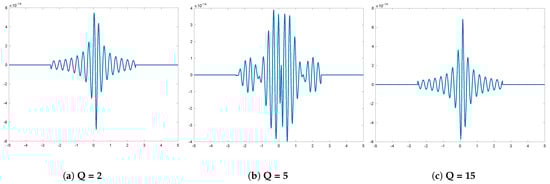
Figure 12. VG* probability density error (${\tilde{f}}_{NQ}\left(x_k\right)-{\tilde{f}}_{QN}\left(x_k\right)$).

7.3. Simulation via the Characteristic Function

The GTS distribution lacks a closed-form probability density function (58), making direct sampling challenging. However, we know the closed form of the Fourier Transform of the density function, $\mathcal{F}\left[f\right]$ (58), and the relationship in (69) provides the Fourier Transform of the cumulative distribution function, $\mathcal{F}\left[F\right]$. The GTS distribution function, $F\left(x\right)$ in (70), was computed from the inverse of the Fourier Transform of the cumulative distribution ($\mathcal{F}\left[F\right]$):  

$$\begin{array}{cc}\hfill Y& \sim GTS(\mu ,{\beta }_{+},{\beta }_{-},{\alpha }_{+},{\alpha }_{-},{\lambda }_{+},f{\lambda }_{-}),\hfill \end{array}$$

(67)

$$\begin{array}{cc}\hfill F\left(x\right)& ={\int }_{-\infty }^{x}f\left(t\right)\mathrm{d}t,f\mathrm{is}\mathrm{the}\mathrm{density}\mathrm{function}\mathrm{of}Y,\hfill \end{array}$$

(68)

$$\begin{array}{cc}\hfill \mathcal{F}\left[F\right]\left(x\right)& ={\displaystyle \frac{\mathcal{F}\left[f\right]\left(x\right)}{ix}}+\pi \mathcal{F}\left[f\right]\left(0\right)\delta \left(x\right),\hfill \end{array}$$

(69)

$$\begin{array}{cc}\hfill F\left(x\right)& ={\displaystyle \frac{1}{2\pi }}{\int }_{-\infty }^{+\infty }{\displaystyle \frac{\mathcal{F}\left[f\right]\left(y\right)}{iy}}{e}^{ixy}\mathrm{d}y+{\displaystyle \frac{1}{2}}.\hfill \end{array}$$

(70)

See Appendix A in [27] for (70) proof.

Theorem 9.

Let a cumulative probability function $F\left(x\right)$ be at least four times continuously differentiable and let ${\left(F_j\right)}_{1\le j\le m}$ be a sample of $F\left(x\right)$ on a sequence of evenly spaced input values ${\left(x_j\right)}_{1\le j\le m}$, with $F\left(x_j\right)=F_j$. We also consider $x_{\alpha }$, a ${\alpha }^{th}$ quantile defined by $F\left(x_{\alpha }\right)=\alpha$, with $x_i<x_{\alpha }<x_{i+1}$ and $F_i<F\left(x_{\alpha }\right)<F_{i+1}$. There exists a unique value, $y\in (0, 1)$, and $b_0$, $b_1$, $b_2$, $b_3$, $b_4$ coefficients such that y is a solution of the polynomial equation of degree 4 (71):

$$b_0+b_{1}y+b_2{y}^2+b_3{y}^3+b_4{y}^4=0.$$

(71)

The ${\alpha }^{th}$ quantile ($x_{\alpha }$) can be written as follows:

$$x_{\alpha }=x_i+y(x_{i+1}-x_i).$$

(72)

Refer to [25] for the proof of Theorem 9.

Given the sample ${\left(F_j\right)}_{1\le j\le m}$ of a cumulative probability function $F\left(x\right)$, Algorithm 6 outlines the inverse transform sampling method.

Algorithm 6 Inverse sampling for a discrete distribution.

1: Input: Parameters ${\alpha }_{+}$, ${\beta }_{+}$, ${\lambda }_{+}$, ${\alpha }_{-}$, ${\beta }_{-}$, ${\lambda }_{-}$, and time horizon $t=1$   2: loop   3:       Initialize: $\mathrm{x}\leftarrow 0$   4:       Draw $u\sim \mathrm{Unif}(0,1)$   5:       if $u=F_i$ then   6:              Accept $x=x_i$ and return to Step 1    (where $F_i=F\left(x_i\right)$)   7:       else   8:             Find i such that $F_i<u<F_{i+1}$   9:             Compute coefficients: $$\begin{array}{c}{b}_0=-(u-F_i),b_1={\displaystyle \frac{F_{i+1}-F_{i-1}}{2}},b_2={\displaystyle \frac{F_{i-1}-2F_i+F_{i+1}}{2}},\hfill \\ b_3={\displaystyle \frac{-F_{i-2}+2F_{i-1}-2F_{i+1}+F_{i+2}}{6}},b_4={\displaystyle \frac{F_{i-2}-4F_{i-1}+6F_i-4F_{i+1}+F_{i+2}}{24}}\end{array}$$ 10:             Solve for $y\in (0,1)$: $b_0+b_{1}y+b_2{y}^2+b_3{y}^3+b_4{y}^4=0$ 11:             Return $x=x_i+y·(x_{i+1}-x_i)$ and return to Step 1 12:       end if 13: end loop

The sampling of daily returns for Bitcoin, Ethereum, the S&P 500 index, and the SPY ETF was performed using the inverse sampling Algorithm 6. Empirical quantiles were computed to construct the Q–Q plots as shown in Figure 13b and Figure 14b.

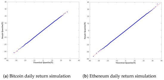
Figure 13. Cryptocurrency daily return simulation: Q-Q Plot with Algorithm 6.

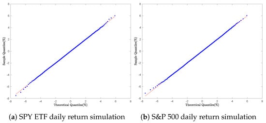
Figure 14. Equity daily return simulation: Q-Q Plot with Algorithm 6.

Graphically, Figure 13a,b and Figure 14a,b. display nearly perfect straight-line relationships; the plotted quantile points fall right on the 45° diagonal. This tight alignment clearly indicates that the simulated samples match the assumed GTS distributions for each asset. In other words, the fit is so accurate that it rules out any meaningful effects from heavy tails or skewness.

The Enhanced FRFT-based inversion sampling method: leveraging the Fast Fractional Fourier Transform (FRFT) combined with high-order Newton–Cotes quadrature rules, this method utilizes the characteristic function to generate highly accurate density estimates for Generalized Tempered Stable (GTS) distributions. This approach achieves

• Superior numerical stability and improved tail accuracy, especially in the presence of heavy-tailed and asymmetric behavior;
• Elimination of truncation and rejection sampling, thereby avoiding common sources of bias and computational inefficiencies inherent in alternative approaches;
• Consistent outperformance relative to existing methods in terms of both theoretical robustness and computational efficiency.

Empirical evaluations confirm the method’s robustness across a range of heavy-tailed and asymmetric distributions, making it particularly well-suited for applications in financial modeling and risk analysis.

8. Goodness-of-Fit Analysis

In addition to the graphical assessment provided by the Q–Q plot, we reinforce our analysis through formal statistical validation using the Kolmogorov–Smirnov (K–S) and Anderson–Darling goodness-of-fit tests. These tests quantitatively evaluate the alignment between the empirical return data and the GTS distribution. By computing test statistics and corresponding p-values, they help determine whether the observed deviations are sufficiently small to consider the GTS model a plausible generator of the return data.

8.1. Kolmogorov–Smirnov (KS) Test

Given a sample of daily returns $\{y_1,y_2,\dots ,y_m\}$ of size m, and the corresponding empirical cumulative distribution function $F_m\left(x\right)$ for each financial asset, the Kolmogorov–Smirnov (KS) test is performed to assess the goodness-of-fit. The null hypothesis $H_0$ assumes that the sample $\{y_1,y_2,\dots ,y_m\}$ is drawn from the GTS distribution with cumulative distribution function $F\left(x\right)$. To carry out the test, the theoretical distribution function $F\left(x\right)$ must be computed explicitly. The two-sided KS goodness-of-fit statistic $D_m$ is defined as

$$\begin{array}{c}\hfill D_m=\underset{x}{sup}\left|F\left(x\right)-F_m\left(x\right)\right|,\end{array}$$

(73)

The distribution of Kolmogorov’s goodness-of-fit statistic, $D_m$, has been extensively studied in the statistical literature. It has been established by Massey [66] that the distribution of $D_m$ is independent of the underlying theoretical cumulative distribution function $F\left(x\right)$, provided the null hypothesis $H_0$ holds, that is, the data sample $\{y_1,y_2,\dots ,y_m\}$ is drawn from a continuous distribution. Extensions to discrete, mixed, and discontinuous distributions have also been addressed in more recent work [67].

Under the null hypothesis $H_0$, it was first shown by Kolmogorov [68] and later refined by Smirnov [69], that the asymptotic distribution of the scaled test statistic $\sqrt{m}{D}_m$ converges to the so-called Kolmogorov distribution as the sample size $m\to \infty$. The cumulative distribution function (CDF) of this limiting distribution is given by the series expansion,

$$\begin{array}{c}\hfill \underset{m\to \infty }{lim}Pr\left(\sqrt{m}{D}_m\le x\right)=1-2\sum _{k=1}^{\infty }{(-1)}^{k-1}{e}^{-2k^2{x}^2}={\displaystyle \frac{\sqrt{2\pi }}{x}}\sum _{k=1}^{\infty }{e}^{-{\displaystyle \frac{{(2k-1)}^2{\pi }^2}{8x^2}}},\end{array}$$

(74)

where the first expression is the classical Kolmogorov series [68], and the second form is derived via the transformation of Jacobi theta functions [70].

As illustrated in Figure 15, the distribution of the asymptotic Kolmogorov statistic $\sqrt{m}{D}_m$ is positively skewed. Marsaglia et al. [70] further analyzed its moments, showing that the mean and standard deviation of this distribution are given by

$$\begin{array}{c}\hfill \mu =\sqrt{{\displaystyle \frac{\pi }{2}}}log\left(2\right)\approx 0.8687,\sigma =\sqrt{{\displaystyle \frac{{\pi }^2}{12}}-{\mu }^2}\approx 0.2603.\end{array}$$

(75)

At $5\%$ risk level, the risk threshold ($d=1.3581$) corresponds to the area in the shaded region under the probability density function.

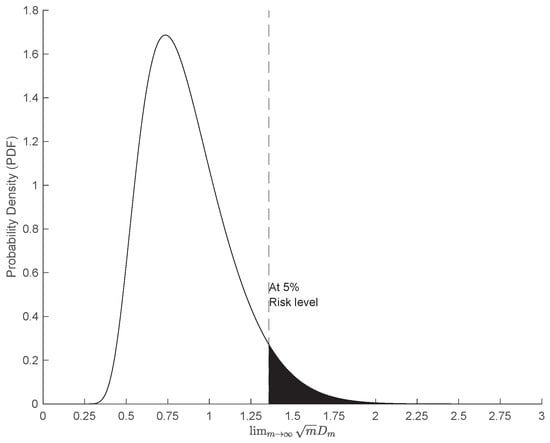
Figure 15. Asymptotic statistic ($\sqrt{m}{D}_m$) PDF.

The KS test is one of the most widely used goodness-of-fit tests based on the empirical distribution function (EDF). It provides a non-parametric method for testing whether a sample comes from a specified continuous distribution. Comprehensive comparisons and applications of EDF-based statistics, including the KS test, can be found in [71,72,73].

To evaluate the test, the p-value associated with the observed KS statistic, ${\widehat{D}}_m$, is calculated using the asymptotic distribution defined in Equation (74). More precisely, the p-value can be expressed as follows:

$$\begin{array}{c}\hfill p_{-}\mathrm{value}=Pr(D_m>{\widehat{D}}_m\mid H_0)=1-Pr\left(\sqrt{m}{D}_m\le \sqrt{m}{\widehat{D}}_m\right).\end{array}$$

(76)

Here, the p-value represents the probability of observing a test statistic as extreme as, or more extreme than, ${\widehat{D}}_m$, under the assumption that the null hypothesis $H_0$ is true. In the context of goodness-of-fit testing, a small p-value (less than 5%) indicates that the empirical distribution $F_m\left(x\right)$ deviates significantly from the theoretical distribution $F\left(x\right)$, casting doubt on the validity of $H_0$.

The value ${\widehat{D}}_m$ represents the observed realization of the KS test statistic $D_m$, computed from the empirical sample $\{y_1,y_2,\dots ,y_m\}$. Following the method described in [74], the estimator ${\widehat{D}}_m$ is defined as

$$\begin{array}{c}\hfill {\widehat{D}}_m=max\left(\underset{0\le j\le P}{sup}\left|F\left(x_j\right)-F_m\left(x_j\right)\right|,\underset{1\le j\le P}{sup}\left|F\left(x_j\right)-F_m\left(x_{j-1}\right)\right|\right).\end{array}$$

(77)

To illustrate the computation, consider the SSR method to sample a Bitcoin (BTC) daily return. KS statistics and the p-values are provided as follows:

$$\begin{array}{cc}\hfill m=80000,{\widehat{D}}_m& =0.0028,p_{-}\mathrm{value}=Pr\left(\sqrt{m}{D}_m>0.7842\mid H_0\right)=57\%.\hfill \end{array}$$

(78)

The p-value of 57% suggests that the null hypothesis $H_0$, that the data follow the theoretical GTS distribution, cannot be rejected at conventional significance levels.

Similar calculations were carried out for the financial asset and the sampling technique. The resulting KS statistics ${\widehat{D}}_m$, $\sqrt{m}{D}_m$ and their corresponding p-values are summarized in Table 6. The KS test results show that the FRFT-based inversion method performed the best, with high p-values (63–99%) across all assets (Bitcoin, Ethereum, S&P 500, SPY ETF), indicating an excellent distributional fit. The Two-Dimensional Single Rejection method showed moderate performance, with p-values ranging from 41% to 72%, while the Inverse Tail Integral approach exhibits greater variability, with p-values ranging from 17% to 72%. In contrast, both the Double Rejection and Shot Noise Representation methods perform poorly, with maximum p-values of just 0.008 and 0.455, respectively, failing to adequately capture the distributional properties. The Standard Stable Rejection method, while acceptable for cryptocurrencies (with p-values ranging from 0.411 to 0.570), proves computationally impractical for equity assets. The findings suggest that Fourier-based methods outperform traditional rejection sampling approaches in both statistical accuracy and computational robustness for Tempered Stable distributions.

Table 6. Kolmogorov–Smirnov test results for different sampling methods.

Financial Assets	Statistics	Exact Sampling Method			Numerical Sampling Method
		SSR 1	Double	Single	Shot	Inverse	Inverse
			Rejection	Rejection 2	Noise 3	Tail Integral 4	Transform 5
Bitcoin	${\widehat{D}}_m$	0.0028	0.0750	0.0025	0.0078	0.0031	0.0019
	$\sqrt{m}{\widehat{D}}_m$	0.7842	21.385	0.7043	2.2045	0.8690	0.5234
	p_value	0.5700	0.0030	0.7041	0.0001	0.4370	0.9470
Ethereum	${\widehat{D}}_m$	0.0031	0.0700	0.0031	0.0030	0.0025	0.0010
	$\sqrt{m}{\widehat{D}}_m$	0.8860	19.865	0.8860	0.8569	0.6935	0.398
	p_value	0.4110	0.0020	0.4110	0.4549	0.7221	0.9970
S&P 500	${\widehat{D}}_m$		0.0836	0.0031	0.1745	0.0039	0.0024
	$\sqrt{m}{\widehat{D}}_m$		23.643	0.8747	49.344	1.1083	0.6811
	p_value		0.0078	0.4286	0.0000	0.1713	0.7424
SPY ETF	${\widehat{D}}_m$		0.0897	0.0025	0.3023	0.0031	0.0026
	$\sqrt{m}{\widehat{D}}_m$		25.366	0.6953	85.498	0.8873	0.7464
	p_value		0.0000	0.7191	0.0000	0.4106	0.6332

¹ Standard Stable Rejection (SSR); ² Two-Dimensional Single Rejection; ³ Shot Noise Representation; ⁴ Inverse Tail Integral Representation; ⁵ Inverse Transform Sampling Scheme.

8.2. Anderson–Darling Test

The Anderson–Darling (AD) test [71,75,76] is a widely used goodness-of-fit test that assesses whether the sample distribution aligns with a specified theoretical distribution. This test belongs to the family of quadratic EDF statistics [72,73], which are designed to quantify the discrepancy between the EDF and the hypothesized CDF. It is mathematically defined as

$$\begin{array}{c}\hfill m{\int }_{-\infty }^{+\infty }{\left(F_m\left(x\right)-F\left(x\right)\right)}^{2}w\left(x\right)dFx,\end{array}$$

(79)

where m is the sample size, $w\left(x\right)$ the weighting function, and $F_m\left(x\right)$ the empirical distribution function defined on the sample size m.

When the weighting function is $w\left(x\right)=1$, the statistic in Equation (79) becomes the Cramér–von Mises statistic [77]. In contrast, the Anderson–Darling statistic [78] is derived by choosing the weighting function $w\left(x\right)=F\left(x\right)(1-F(x\left)\right)$, where $F\left(x\right)$ is the hypothesized cumulative distribution function. The key difference between the two statistics lies in the weighting applied to the data. Specifically, the Anderson–Darling (AD) statistic places more weight on the tails of the distribution, making it more sensitive to deviations in the extreme values compared to the Cramér–von Mises statistic, which treats the distribution more uniformly across the entire range. The AD statistic is mathematically defined as

$$\begin{array}{cc}\hfill A_m^2& =m{\int }_{-\infty }^{+\infty }{\displaystyle \frac{{\left(F_m\left(x\right)-F\left(x\right)\right)}^2}{F\left(x\right)\left(1-F\left(x\right)\right)}}dF\left(x\right).\hfill \end{array}$$

(80)

It can be shown that the asymptotic distribution of the AD statistic, $A_m^2$, is independent of the theoretical distribution under the null hypothesis. The asymptotic distribution [79,80,81] is defined as follows:

$$\begin{array}{cc}\hfill G\left(x\right)& =\underset{m\to \infty }{lim}Pr\left[A_m^2<x\right]=\sum _{j=0}^{\infty }{a}_j{\left(x{b}_j\right)}^{-{\displaystyle \frac{1}{2}}}exp\left(-{\displaystyle \frac{b_j}{x}}\right){\int }_0^{\infty }{f}_j\left(y\right)exp(-y^2)dy,\hfill \\ \hfill f_j\left(y\right)& =exp\left({\displaystyle \frac{1}{8}}{\displaystyle \frac{x{b}_j}{y^{2}x+b_j}}\right),\hfill \\ \hfill a_j& ={\displaystyle \frac{{(-1)}^j{\left(2\right)}^{\frac{1}{2}}(4j+1)\mathrm{\Gamma }\left(j+\frac{1}{2}\right)}{j!}},\hfill \\ \hfill b_j& ={\displaystyle \frac{1}{2}}{(4j+1)}^2{\pi }^2.\hfill \end{array}$$

(81)

As shown in Figure 16, the asymptotic distribution of the Anderson–Darling statistic, $A_m^2$, is positively skewed, with a mean and standard deviation [76,82] defined as follows:

$$\begin{array}{cc}\hfill \mu & =1,\sigma =\sqrt{{\displaystyle \frac{2}{3}}\left({\pi }^2-9\right)}\sim 0.761.\hfill \end{array}$$

(82)

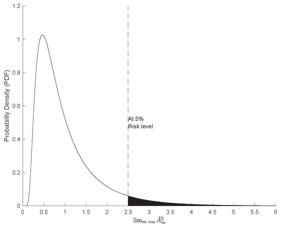
Figure 16. Asymptotic Anderson–Darling (AD) statistic ($A_m^2$) PDF.

At a 5% risk level, the associated risk threshold ($d=2.4941$) corresponds to the area in the shaded region under the probability density function. The p-value of the test statistic, $A_m^2$, is defined as follows:

$$\begin{array}{c}\hfill p\text{-}value=prob(A_m^2>{\widehat{A}}_m^2|H_0)=1-G\left({\widehat{A}}_m^2\right).\end{array}$$

(83)

To compute the AD statistic, $A_m^2$, in Equation (80), the sample of daily returns $\{y_1,y_2,\dots ,y_m\}$ of size m is arranged in ascending order:

$$y_{\left(1\right)}<y_{\left(2\right)}<\dots <y_{\left(m\right)}.$$

The Anderson–Darling statistic [80] is then computed as follows:

$$\begin{array}{c}\hfill A_m^2=-m-{\displaystyle \frac{1}{m}}\sum _{j=1}^m\left[(2j-1)log\left(F\left(y_{\left(j\right)}\right)\right)+(2(m-j)+1)log(1-F\left(y_{\left(j\right)}\right))\right].\end{array}$$

(84)

For each financial asset, and each sampling method, the AD statistic, as defined in Equation (84), is computed along with the corresponding p-value statistic, as shown in Table 7. The AD test results show performance differences among sampling methods. The FRFT-based inversion method leads, with p-values exceeding 94% for Bitcoin, Ethereum, and the S&P 500, and 54% for the SPY ETF, demonstrating unmatched accuracy in GTS distributions. The Inverse Tail Integral method appears promising for Ethereum (97% p-value) but underperforms elsewhere (p-values between 43% and 49%). The Two-Dimensional Single Rejection method yields modest results (p-values from 55% to 71%), while the Standard Stable Rejection method is mostly effective with cryptocurrencies (74% to 76%). Both the Double Rejection and Shot Noise methods fail, with 0% p-values for most assets. Like the KS test, the AD results emphasize the FRFT method as the most reliable for capturing heavy-tailed behavior in financial data.

Table 7. Anderson–Darling test results for different sampling methods.

Financial Assets	Statistics	Exact Sampling Method			Numerical Sampling Method
		SSR 1	Double	Single	Shot	Inverse	Inverse
			Rejection	Rejection 2	Noise 3	Tail Integral 4	Transform 5
Bitcoin	${\widehat{A}}_m^2$	0.4850	496.5	0.6049	3.299	0.8677	0.2876
	p_value	0.7622	0.0000	0.6434	0.0194	0.4347	0.9472
Ethereum	${\widehat{A}}_m^2$	0.4993	428.8	0.7051	0.9525	0.2579	0.2464
	p_value	0.7475	0.0000	0.5545	0.3832	0.9660	0.9722
S&P 500	${\widehat{A}}_m^2$		621.5	0.6816	5292	0.8244	0.2924
	p_value		0.0000	0.5744	0.0000	0.4638	0.9438
SPY ETF	${\widehat{A}}_m^2$		658.4	0.5409	1522	0.7834	0.7232
	p_value		0.0000	0.7055	0.0000	0.4932	0.5397

¹ Standard Stable Rejection (SSR); ² Two-Dimensional Single Rejection; ³ Shot Noise Representation; ⁴ Inverse Tail Integral Representation; ⁵ Inverse Transform Sampling Scheme.

9. Conclusions

This paper addressed the challenge of simulating random variates from the Generalized Tempered Stable (GTS) distribution, a flexible framework for modeling heavy-tailed data. While GTS models are theoretically powerful, their lack of closed-form densities has limited practical simulation. We provided a comprehensive and systematic comparison of existing simulation techniques, spanning rejection-based algorithms, series representations, and numerical inversion methods.

Our findings demonstrate that classical rejection algorithms, such as the Standard Stable Rejection and Double Rejection methods, have theoretical value. However, they exhibit poor performance under extreme parameter conditions (${\lambda }_{\pm }\to +\infty ,{\beta }_{\pm }\to 0$). While enhanced variants like the Double Rejection method demonstrate improved efficiency, they still fall short in accurately capturing tail behavior—a critical requirement for risk-sensitive financial applications. Similarly, the series representation techniques, such as the Shot Noise series representation, provide valuable theoretical insights into GTS processes but exhibit numerical instability when dealing with extreme parameter values, limiting their practical utility.

The comparative evaluation identifies three particularly effective methods: the Two-Dimensional Single Rejection technique, the inverse Lévy measure series representation, and the Fast Fractional Fourier Transform (FRFT)-based inversion approach. Among these methods, the Enhanced Fast Fractional Fourier Transform (FRFT)-based inversion method, consistently achieves the highest accuracy in goodness-of-fit tests (Kolmogorov–Smirnov and Anderson–Darling) across all tested assets—Bitcoin, Ethereum, the S&P 500, and the SPY ETF—while maintaining competitive computational efficiency. This positions the FRFT approach as the most reliable and versatile option for GTS simulation, particularly in risk-sensitive financial applications where accurate tail modeling is essential. Our research contributes to the literature in three main ways. First, it offers a unified and systematic comparison of available GTS simulation methods, clearly articulating their respective strengths and limitations. Second, it introduces an enhanced FRFT-based algorithm that sets a new standard for accurate and efficient GTS simulations. Third, it highlights practical implications for financial modeling, where capturing tail risk with high fidelity is essential.

The development of efficient simulation methods for multivariate GTS distributions remains a crucial challenge. Future research should focus on extending the FRFT approach to higher dimensions while preserving computational efficiency. This advancement would facilitate more realistic modeling of portfolio risk and the dependence structures among financial assets.

References

- Cont, R.; Tankov, P. Financial Modelling with Jump Processes; Chapman & Hall/CRC: Boca Raton, FL, USA, 2004. [Google Scholar]
- Samorodnitsky, G.; Taqqu, M.S. Stable Non-Gaussian Random Processes: Stochastic Models with Infinite Variance; CRC Press: New York, NY, USA, 1994. [Google Scholar]
- Nzokem, A.H. Comparing Bitcoin and Ethereum Tail Behavior via QQ Analysis of Cryptocurrency Returns. arXiv 2025, arXiv:2507.01983. [Google Scholar]
- Nolan, J.P. Univariate Stable Distributions: Models for Heavy Tailed Data; Springer Series in Operations Research and Financial Engineering: Cham, Switzerland, 2020. [Google Scholar] [CrossRef]
- Rosiński, J. Tempering Stable Processes. Stoch. Process. Their Appl. 2007, 117, 677–707. [Google Scholar] [CrossRef]
- Küchler, U.; Tappe, S. Tempered Stable Distributions and Processes. Stoch. Process. Their Appl. 2013, 123, 4256–4293. [Google Scholar] [CrossRef]
- Carr, P.; Geman, H.; Madan, D.B.; Yor, M. Stochastic Volatility for Lévy Processes. Math. Financ. 2003, 13, 345–382. [Google Scholar] [CrossRef]
- Rachev, S.T.; Kim, Y.S.; Bianchi, M.L.; Fabozzi, F.J. Stable and Tempered Stable Distributions. In Financial Models with Lévy Processes and Volatility Clustering; The Frank J. Fabozzi Series; Rachev, S.T., Kim, Y.S., Bianchi, M.L., Fabozzi, F.J., Eds.; John Wiley & Sons: Hoboken, NJ, USA, 2011; Volume 187, pp. 57–85. [Google Scholar] [CrossRef]
- Boyarchenko, S.I.; Levendorskiĭ, S.Z. Non-Gaussian Merton-Black-Scholes Theory; Advanced Series on Statistical Science & Applied Probability; World Scientific: Singapore, 2002; Volume 9. [Google Scholar] [CrossRef]
- Küchler, U.; Tappe, S. Bilateral Gamma Distributions and Processes in Financial Mathematics. Stoch. Process. Their Appl. 2008, 118, 261–283. [Google Scholar] [CrossRef]
- Nzokem, A.H. Self-Decomposable Laws Associated with General Tempered Stable (GTS) Distribution and Their Simulation Applications. arXiv 2024, arXiv:2405.16614. [Google Scholar] [CrossRef]
- Devroye, L. Random Variate Generation for Exponentially and Polynomially Tilted Stable Distributions. ACM Trans. Model. Comput. Simul. 2009, 19, 1–20. [Google Scholar] [CrossRef]
- Glasserman, P. Generating Random Numbers and Random Variables. In Monte Carlo Methods in Financial Engineering; Springer: New York, NY, USA, 2003; pp. 39–77. [Google Scholar] [CrossRef]
- Qu, Y.; Dassios, A.; Zhao, H. Random Variate Generation for Exponential and Gamma Tilted Stable Distributions. ACM Trans. Model. Comput. Simul. 2021, 31, 1–21. [Google Scholar] [CrossRef]
- Dassios, A.; Qu, Y.; Zhao, H. Exact simulation for a class of tempered stable and related distributions. ACM Trans. Model. Comput. Simul. (TOMACS) 2018, 28, 1–21. [Google Scholar] [CrossRef]
- Hofert, M. Sampling Exponentially Tilted Stable Distributions. ACM Trans. Model. Comput. Simul. 2011, 22, 3. [Google Scholar] [CrossRef]
- Nzokem, A.H.; Maposa, D. Exact Simulation for General Tempered Stable Random Variates: Review and Empirical Analysis. In Proceedings of the 2025 International Conference on Artificial Intelligence, Computer, Data Sciences and Applications (ACDSA), Antalya, Turkiye, 7–9 August 2025; IEEE: Piscataway, NJ, USA, 2025; pp. 1–6. [Google Scholar] [CrossRef]
- Rosiński, J. Tempered Stable Processes. In Proceedings of the Second MaPhySto Conference on Lévy Processes: Theory and Applications, Aarhus, Denmark, 21–25 January 2002; Volume 22, pp. 215–220. Available online: http://www.maphysto.dk/publications/MPS-misc/2002/22.pdf (accessed on 20 May 2025).
- Rosiński, J. Series Representations of Lévy Processes from the Perspective of Point Processes. In Lévy Processes: Theory and Applications; Barndorff-Nielsen, O.E., Resnick, S.I., Mikosch, T., Eds.; Birkhäuser: Boston, MA, USA, 2001; pp. 401–415. [Google Scholar] [CrossRef]
- Shephard, N. From Characteristic Function to Distribution Function: A Simple Framework for the Theory. Econom. Theory 1991, 7, 519–529. [Google Scholar] [CrossRef]
- Nzokem, A.; Maposa, D.; Seimela, A.M. Enhanced Fast Fractional Fourier Transform (FRFT) Scheme Based on Closed Newton-Cotes Rules. Axioms 2025, 14, 543. [Google Scholar] [CrossRef]
- Kyprianou, A.E. Fluctuations of Lévy Processes with Applications: Introductory Lectures; Universitext; Springer: Berlin/Heidelberg, Germany, 2014. [Google Scholar]
- Sato, K.I. Basic Results on Lévy Processes. In Lévy Processes: Theory and Applications; Barndorff-Nielsen, O.E., Mikosch, T., Resnick, S.I., Eds.; Birkhäuser: Boston, MA, USA, 2001; pp. 1–37. [Google Scholar] [CrossRef]
- Tankov, P. Financial Modeling with Lévy Processes: Lecture Notes. 2010. Available online: https://cel.hal.science/cel-00665021v1 (accessed on 20 May 2025).
- Nzokem, A.H.; Maposa, D. Bitcoin versus S&P 500 Index: Return and Risk Analysis. Math. Comput. Appl. 2024, 29, 44. [Google Scholar] [CrossRef]
- Nzokem, A.; Maposa, D. Fitting the Seven-Parameter Generalized Tempered Stable Distribution to Financial Data. J. Risk Financ. Manag. 2024, 17, 531. [Google Scholar] [CrossRef]
- Nzokem, A.H. Fitting Infinitely Divisible Distribution: Case of Gamma-Variance Model. arXiv 2021, arXiv:2104.07580. [Google Scholar] [CrossRef]
- Nzokem, A.H. Five-Parameter Variance-Gamma Process: Lévy versus Probability Density. AIP Conf. Proc. 2024, 3005, 020030. [Google Scholar] [CrossRef]
- Nzokem, A.H.; Montshiwa, V.T. Fitting Generalized Tempered Stable Distribution: Fractional Fourier Transform (FRFT) Approach. arXiv 2022, arXiv:2205.00586. [Google Scholar] [CrossRef]
- Nzokem, A.H. Gamma Variance Model: Fractional Fourier Transform (FRFT). J. Physics Conf. Ser. 2021, 2090, 012094. [Google Scholar] [CrossRef]
- Nzokem, A.H. Pricing European options under stochastic volatility models: Case of five-parameter variance-gamma process. J. Risk Financ. Manag. 2023, 16, 55. [Google Scholar] [CrossRef]
- Uchaikin, V.V.; Zolotarev, V.M. Chance and Stability: Stable Distributions and their Applications; Modern Probability and Statistics; De Gruyter: Berlin, Germany, 2011. [Google Scholar]
- Zolotarev, V.M. One-Dimensional Stable Distributions; American Mathematical Society: Providence, RI, USA, 1986; Volume 65. [Google Scholar]
- Feller, W. An Introduction to Probability Theory and Its Applications, 2nd ed.; John Wiley & Sons: New York, NY, USA, 1971; Volume 2. [Google Scholar]
- Kring, S.; Rachev, S.T.; Höchstötter, M.; Fabozzi, F.J. Estimation of α-stable sub-Gaussian distributions for asset returns. In Risk Assessment: Decisions in Banking and Finance; Springer: Berlin/Heidelberg, Germany, 2009; pp. 111–152. [Google Scholar]
- Zolotarev, V.M. On the Representation of Stable Laws by Integrals. Tr. Mat. Instituta Im. V. A. Steklova 1964, 71, 46–50. [Google Scholar]
- Borak, S.; Härdle, W.; Weron, R. Stable Distributions. In Statistical Tools for Finance and Insurance; Springer: Berlin/Heidelberg, Germany, 2005; pp. 21–44. [Google Scholar] [CrossRef]
- Box, G.E.P.; Muller, M.E. A Note on the Generation of Random Normal Deviates. Ann. Math. Stat. 1958, 29, 610–611. [Google Scholar] [CrossRef]
- Chambers, J.M.; Mallows, C.L.; Stuck, B.W. A Method for Simulating Stable Random Variables. J. Am. Stat. Assoc. 1976, 71, 340–344. [Google Scholar] [CrossRef]
- Barndorff-Nielsen, O.E.; Shephard, N. Financial Volatility, Lévy Processes and Power Variation. 2002. Available online: https://www.olsendata.com/data_products/client_papers/papers/200206-NielsenShephard-FinVolLevyProcessPowerVar.pdf (accessed on 20 May 2025).
- Brix, A. Generalized Gamma Measures and Shot-Noise Cox Processes. Adv. Appl. Probab. 1999, 31, 929–953. [Google Scholar] [CrossRef]
- Ripley, B.D. Stochastic Simulation; John Wiley & Sons: New York, NY, USA, 2009. [Google Scholar]
- Hofert, M. Efficiently Sampling Nested Archimedean Copulas. Comput. Stat. Data Anal. 2011, 55, 57–70. [Google Scholar] [CrossRef]
- Cerquetti, A. A Note on Bayesian Nonparametric Priors Derived from Exponentially Tilted Poisson-Kingman Models. Stat. Probab. Lett. 2007, 77, 1705–1711. [Google Scholar] [CrossRef]
- Nzokem, A.H. Numerical Solution of a Gamma-Integral Equation Using a Higher Order Composite Newton-Cotes Formulas. J. Phys. Conf. Ser. 2021, 2084, 012019. [Google Scholar] [CrossRef]
- Nzokem, A.H. Stochastic and Renewal Methods Applied to Epidemic Models. Ph.D. Thesis, York University, Toronto, ON, Canada, 2020. [Google Scholar]
- Nzokem, A.H. European Option Pricing Under Generalized Tempered Stable Process: Empirical Analysis. arXiv 2023, arXiv:2304.06060. [Google Scholar] [CrossRef]
- Nzokem, A.H.; Montshiwa, V.T. The Ornstein-Uhlenbeck Process and Variance Gamma Process: Parameter Estimation and Simulations. Thai J. Math. 2023, 160–168. [Google Scholar]
- Loy, A.; Follett, L.; Hofmann, H. Variations of Q-Q Plots: The Power of Our Eyes! Am. Stat. 2016, 70, 202–214. [Google Scholar] [CrossRef]
- Thode, H.C. Testing for Normality; Statistics, Textbooks and Monographs; CRC Press: New York, NY, USA, 2002; Volume 164. [Google Scholar]
- Wang, M.C.; Bushman, B.J. Using the Normal Quantile Plot to Explore Meta-Analytic Data Sets. Psychol. Methods 1998, 3, 46–54. [Google Scholar] [CrossRef]
- Wilk, M.B.; Gnanadesikan, R. Probability Plotting Methods for the Analysis of Data. Biometrika 1968, 55, 1–17. [Google Scholar] [CrossRef]
- Dodge, Y. Q-Q Plot (Quantile to Quantile Plot). In The Concise Encyclopedia of Statistics; Springer: New York, NY, USA, 2008; pp. 437–439. [Google Scholar] [CrossRef]
- Rachev, S.T. Tempered Stable Models in Finance: Theory and Applications. Ph.D. Thesis, University of Bergamo, Bergamo, Italy, 2009. [Google Scholar]
- Ivanenko, D.; Knopova, V.; Platonov, D. On Approximation of Some Lévy Processes. Austrian J. Stat. 2025, 54, 177–199. [Google Scholar] [CrossRef]
- Kallenberg, O. Foundations of Modern Probability; Springer: New York, NY, USA, 1997; Volume 2. [Google Scholar]
- Ferguson, T.S.; Klass, M.J. A Representation of Independent Increment Processes Without Gaussian Components. Ann. Math. Stat. 1972, 43, 1634–1643. [Google Scholar] [CrossRef]
- Nzokem, A. Simulation of Generalized Tempered Stable (GTS) Random Variates via Series Representations: A Case Study of Bitcoin and Ethereum. Preprint 2025. [Google Scholar] [CrossRef]
- Yuan, S.; Kawai, R. Numerical aspects of shot noise representation of infinitely divisible laws and related processes. Probab. Surv. 2021, 18, 201–271. [Google Scholar] [CrossRef]
- Godsill, S.; Kontoyiannis, I.; Tapia Costa, M. Generalised shot-noise representations of stochastic systems driven by non-Gaussian Lévy processes. Adv. Appl. Probab. 2024, 56, 1215–1250. [Google Scholar] [CrossRef]
- Gil-Pelaez, J. Note on the Inversion Theorem. Biometrika 1951, 38, 481–482. [Google Scholar] [CrossRef]
- Carr, P.; Madan, D.B. Option Valuation Using the Fast Fourier Transform. J. Comput. Financ. 1999, 2, 61–73. [Google Scholar] [CrossRef]
- Fang, F.; Oosterlee, C.W. A Novel Pricing Method for European Options Based on Fourier-Cosine Series Expansions. SIAM J. Sci. Comput. 2008, 31, 826–848. [Google Scholar] [CrossRef]
- Bailey, D.H.; Swarztrauber, P.N. The Fractional Fourier Transform and Applications. SIAM Rev. 1991, 33, 389–404. [Google Scholar] [CrossRef]
- Bailey, D.H.; Swarztrauber, P.N. A Fast Method for the Numerical Evaluation of Continuous Fourier and Laplace Transforms. SIAM J. Sci. Comput. 1994, 15, 1105–1110. [Google Scholar] [CrossRef]
- Massey, F.J. The Kolmogorov-Smirnov Test for Goodness of Fit. J. Am. Stat. Assoc. 1951, 46, 68–78. [Google Scholar] [CrossRef]
- Dimitrova, D.S.; Kaishev, V.K.; Tan, S. Computing the Kolmogorov-Smirnov Distribution When the Underlying CDF is Purely Discrete, Mixed, or Continuous. J. Stat. Softw. 2020, 95, 1–42. [Google Scholar] [CrossRef]
- Kolmogorov, A.N. Sulla Determinazione Empirica di una Legge di Distribuzione. G. Dell’Istituto Ital. Degli Attuari 1933, 4, 83–91. [Google Scholar]
- Smirnov, N.V. Table for Estimating the Goodness of Fit of Empirical Distributions. Ann. Math. Stat. 1948, 19, 279–281. [Google Scholar] [CrossRef]
- Marsaglia, G.; Tsang, W.W.; Wang, J. Evaluating Kolmogorov’s Distribution. J. Stat. Softw. 2003, 8, 1–4. [Google Scholar] [CrossRef]
- D’Agostino, R.B.; Stephens, M.A. Goodness-of-Fit Techniques; Marcel Dekker: New York, NY, USA, 1986. [Google Scholar]
- Stephens, M.A. EDF Statistics for Goodness of Fit and Some Comparisons. J. Am. Stat. Assoc. 1974, 69, 730–737. [Google Scholar] [CrossRef]
- Shorack, G.R.; Wellner, J.A. Empirical Processes with Applications to Statistics; John Wiley & Sons: New York, NY, USA, 1986. [Google Scholar]
- Krysicki, W.; Bartos, J.; Dyczka, W.; Królikowska, K.; Wasilewski, M. Rachunek Prawdopodobieństwa i Statystyka Matematyczna w zadaniach; Wydawnictwo Naukowe PWN: Warszawa, Poland, 1999; Volume 2. [Google Scholar]
- Anderson, T.W. Anderson-Darling Test. In The Concise Encyclopedia of Statistics; Dodge, Y., Ed.; Springer: New York, NY, USA, 2008; pp. 12–14. [Google Scholar] [CrossRef]
- Anderson, T.W.; Darling, D.A. A Test of Goodness of Fit. J. Am. Stat. Assoc. 1954, 49, 765–769. [Google Scholar] [CrossRef]
- von Mises, R. Wahrscheinlichkeit, Statistik und Wahrheit; Julius Springer: Berlin/Heidelberg, Germany, 1931; English translation: Probability, Statistics and Truth, Macmillan, 1957. [Google Scholar]
- Anderson, T.W.; Darling, D.A. Asymptotic Theory of Certain “Goodness of Fit” Criteria Based on Stochastic Processes. Ann. Math. Stat. 1952, 23, 193–212. [Google Scholar] [CrossRef]
- Durbin, J. Distribution Theory for Tests Based on the Sample Distribution Function; SIAM: Philadelphia, PA, USA, 1973. [Google Scholar]
- Lewis, P.A.W. Distribution of the Anderson-Darling Statistic. Ann. Math. Stat. 1961, 32, 1118–1124. [Google Scholar] [CrossRef]
- Marsaglia, G.; Marsaglia, J. Evaluating the Anderson-Darling Distribution. J. Stat. Softw. 2004, 9, 1–5. [Google Scholar] [CrossRef]
- Anderson, T.W. Anderson-Darling Tests of Goodness-of-Fit. In International Encyclopedia of Statistical Science; Lovric, M., Ed.; Springer: Berlin/eidelberg, Germany, 2011; pp. 52–54. [Google Scholar] [CrossRef]
Disclaimer/Publisher’s Note: The statements, opinions and data contained in all publications are solely those of the individual author(s) and contributor(s) and not of MDPI and/or the editor(s). MDPI and/or the editor(s) disclaim responsibility for any injury to people or property resulting from any ideas, methods, instructions or products referred to in the content. |
© 2025 by the authors. Licensee MDPI, Basel, Switzerland. This article is an open access article distributed under the terms and conditions of the Creative Commons Attribution (CC BY) license (https://creativecommons.org/licenses/by/4.0/).