Article

Application of the Kurganov–Tadmor Scheme in Curvilinear Coordinates for Supersonic Flow

by
Sebastián Bertolo
1,
Sergio Elaskar
1,2,* and
Luis Gutiérrez Marcantoni
1
1
Department of Aerospace Engineering, Faculty of Exact, Physical and Natural Sciences, National University of Cordoba, Córdoba 5000, Argentina
2
Institute of Advanced Studies in Engineering and Technology (IDIT), CONICET and National University of Cordoba, Córdoba 5000, Argentina
*
Author to whom correspondence should be addressed.
Math. Comput. Appl. 2025, 30(5), 92; https://doi.org/10.3390/mca30050092
Submission received: 21 June 2025 / Revised: 15 August 2025 / Accepted: 21 August 2025 / Published: 23 August 2025
(This article belongs to the Special Issue Feature Papers in Mathematical and Computational Applications 2025)

Abstract

In this current study, we developed a second-order Kurganov–Tadmor scheme in curvilinear coordinates to analyze the external supersonic flow over bodies of various shapes. This scheme is capable of handling interfaces across different regions of the domain. We utilized a fourth-order Runge–Kutta temporal integrator and conducted several test cases to validate the performance of the new scheme. The results from the analyzed tests indicate that the new method produces highly accurate outcomes.

1. Introduction

Supersonic flow plays a critical role in aerospace engineering, with applications in both internal and external aerodynamics. The determination of high-velocity flow properties around bodies has been the focus of extensive theoretical, numerical, and experimental studies [1,2,3,4,5,6].
Computational Fluid Dynamics (CFD) simulations are increasingly employed to analyze supersonic flows [6,7,8,9,10,11]. The selection of the numerical method is pivotal in these simulations. One widely used scheme is the one developed by Kurganov and Tadmor, which is extensively cited in the scientific literature [12,13,14,15,16,17,18]. This central scheme is independent of the problem’s eigenstructure and utilizes precise information on local propagation velocities. It also represents the non-smooth part of the solution in terms of its cell averages integrated over Riemann fans of different sizes. Also, in Ref. [12], the authors have demonstrated that the scalar version of the Kurganov–Tadmor high-resolution central scheme is non-oscillatory. It satisfies the total-variation diminishing property in the one-dimensional case and the maximum principle in two-dimensional domains.
The Kurganov and Tadmor method has demonstrated robustness and effectiveness in simulating systems of hyperbolic equations [12]. By applying this method in curvilinear coordinates, it is possible to adapt more effectively to complex geometries that are often encountered in external flow problems [14]. Furthermore, the use of meshes with varying topologies provides flexibility in discretizing the study domain, which is crucial for accurately capturing the flow details in specific regions of interest.
The original development of the Kurganov–Tadmor scheme was for a Cartesian coordinate system [12]. Consequently, studies involving bodies of arbitrary geometry often utilized meshes with non-orthogonal element distributions. This study investigates the implementation of the Kurganov and Tadmor method in curvilinear coordinates for simulating external supersonic flows. A new methodology is introduced to enable the use of meshes with different topologies, thereby facilitating the optimal treatment of the interfaces between them. The validity of this methodology is confirmed through solutions of the well-established Euler equations [2], employing a fourth-order Runge–Kutta temporal integrator [19]. We introduce a second-order central scheme designed for systems of hyperbolic conservation laws on curvilinear grids, which builds upon previous work by [14]. At the core of our methodology is the ability to partition the domain into multiple subdomains and a novel approach for handling the interfaces between these subdomains. Additionally, the new method shows second-order accuracy, delivering more precise results compared to the traditional Kurganov–Tadmor–Petrova (KNP) scheme. This advancement not only improves precision but also enhances the reliability of outcomes.
The Euler equations are a set of nonlinear hyperbolic differential equations that delineate the flow of compressible gas without accounting for mass forces, viscosity, and heat transfer by radiation and conduction [2,20,21]. Although this work particularly focuses on solving these equation systems, the scheme presented here can be extended to other types of governing equations formulated in curvilinear coordinates, such as the Burger equation [9].
This work is divided into four sections, starting with the introduction. Section 2 elaborates on the numerical method used, its application, treatment of region interfaces, and the time step condition. Section 3 details the cases to be analyzed, including a cylinder, a wedge, and a blunt body, along with the obtained results. Finally, Section 4 presents the conclusions drawn from this work.

2. Numerical Method

In this section, we present the numerical scheme developed in this study. First, we outline the fundamental equations: the two-dimensional Euler equations in curvilinear coordinates. Next, we introduce the Kurganov–Tadmor scheme. The following subsection presents the temporal scheme used to solve the equation system over time, and finally, we describe the interface treatment.

2.1. Fundamental Equations

In our analysis of non-viscous supersonic flow, we will be focusing on the two-dimensional Euler equations due to their widespread use.
The Euler equations are derived from the Navier–Stokes equations [22] by neglecting diffusive effects. They are used to describe the flow of fluid in which thermal conductivity and viscosity are not significant. These fluids are referred to as ideal fluids [20]. While we refer the reader to fluid mechanics books for their development and properties in Cartesian coordinates, we also recommend consulting references [9,20].
For our current work, we are exploring the presentation of these equations concerning an arbitrary curvilinear coordinate system. This involves utilizing a general coordinate transformation
x = x ( ξ , η ) y = y ( ξ , η ) .
The two-dimensional unsteady Euler equations in curvilinear coordinates can be written as [23]
ρ t + 1 h ξ h η ξ h η ρ u ξ + 1 h ξ h η η h ξ ρ u η = 0
ρ u ξ t + 1 h ξ h η ξ h η ρ u ξ 2 + p + 1 h ξ h η η h ξ ρ u η u ξ = 1 h ξ h η h η ξ ρ u η 2 + p ρ u ξ u η h ξ h η h ξ η
ρ u η t + 1 h ξ h η ξ h η ρ u ξ u η + 1 h ξ h η η h ξ ρ u η 2 + p = 1 h ξ h η h ξ ξ ρ u ξ 2 + p ρ u ξ u η h ξ h η h η ξ
E t + 1 h ξ h η ξ h η u ξ E + p + 1 h ξ h η η h ξ u η E + p = 0 .
where h ξ and h η are the transformation scale factors, which are defined according to the coordinate systems. Also, ρ is the density, p the pressure, E the energy, and ( u ξ , u η ) the velocity vector.
The used state equation is that of a perfect gas
ρ = p R T ,
where R is the gas constant, and T the temperature. Therefore, the energy can be defined as
E = 1 2 ρ u ξ 2 + u η 2 + p γ 1 .
The previous set of equations in matrix form results in
U t + 1 h ξ h η ξ h η F ( U ) + 1 h ξ h η ξ h ξ G ( U ) = S ( U ) ,
where U = ( ρ , ρ u ξ , ρ u η , E ) T is the vector of conservative variables. F ( U ) and G ( U ) are the flow vectors, and S ( U ) is the source term.
The system given by Equation (5) is conservative, allowing the application of the numerical method introduced here.

2.2. Kurganov–Tadmor Scheme

The numerical scheme here employed to solve the system of equations described in the previous subsection is the one developed by Kurganov and Tadmor. This scheme was described in Ref. [12].
Every numerical method involves discretizing the continuous governing equations to calculate variables at specific discrete points within the domain, known as nodes. To accomplish this, the domain is divided into small control volumes or cells. In the case of this two-dimensional scheme, surfaces are utilized, and nodes are positioned at their centers. The node within each cell represents the average value of the variable over the entire cell
U ¯ ( ξ , η , t ) = 1 V ξ , η V ξ , η U ( ξ , η , t ) h ξ h η d ξ d η ,
where the V ξ . η corresponds to the surface of each cell. The evaluation of this surface will be explained in the next paragraphs. Therefore, Equation (5) is integrated in a domain V ξ , η x [ t , t + Δ t ]
U ¯ ( ξ , η , t + Δ t ) = U ¯ ( ξ , η , t ) + t t + Δ t 1 h ξ h η ξ h η F ( U ) ¯ + 1 h ξ h η η h ξ G ( U ) ¯ S ( U ) ¯ d t .
To evaluate the integral equation, each cell is subdivided into smaller regions based on the impact of the Riemann problem on each interface. To determine the value of the variable at the interface, a Riemann problem is solved, which indicates that within a time interval Δ t , the waves will influence specific portions of the cell. This scheme is illustrated in Figure 1 for a two-dimensional domain. It is important to note that regions near the edges receive influence from neighboring cells [13].
We assume that the variables have a linear distribution within each cell. Therefore, their value can be calculated as
U ˜ i , j n ( ξ , η ) = U ¯ i , j n + u ξ i , j n ( ξ ξ i , j ) + u η i , j n ( η η i , j ) .
In this equation, u ξ and u η are the velocity derivatives in each direction; the calculation of these derivatives will be detailed later.
The coordinates that define each subdomain are obtained according to
ξ e ± = ξ i + 1 2 , j + a i + 1 2 , j ± Δ t h ξ ( ξ i + 1 2 , η j ) ξ w ± = ξ i 1 2 , j + a i 1 2 , j ± Δ t h ξ ( ξ i 1 2 , η j ) η n ± = η i , j + 1 2 + b i , j + 1 2 ± Δ t h η ( ξ i , η j + 1 2 ) η s ± = η i , j 1 2 + b i , j 1 2 ± Δ t h η ( ξ i , η j 1 2 ) .
where a and b are the local velocities at the interfaces; in practice, they can be determined as
a i + 1 2 , j + = m a x λ m a x F U U i + 1 2 , j + , λ m a x F U U i + 1 2 , j a i + 1 2 , j = m i n λ m i n F U U i + 1 2 , j + , λ m i n F U U i + 1 2 , j b i , j + 1 2 + = m a x λ m a x G U U i , j + 1 2 + , λ m a x G U U i , j + 1 2 b i , j + 1 2 = m i n λ m i n G U U i , j + 1 2 + , λ m i n G U U i , j + 1 2 .
For the edges, there is the influence of waves coming from neighboring interfaces. Therefore, the velocities can be calculated as
A i ± 1 2 , j + 1 2 + = m a x a i ± 1 2 , j + , a i ± 1 2 , j + 1 + A i ± 1 2 , j + 1 2 = m i n a i ± 1 2 , j , a i ± 1 2 , j + 1 A i ± 1 2 , j 1 2 + = m a x a i ± 1 2 , j + , a i ± 1 2 , j 1 + A i ± 1 2 , j 1 2 = m i n a i ± 1 2 , j , a i ± 1 2 , j 1 B i + 1 2 , j ± 1 2 + = m a x b i , j ± 1 2 + , b i + 1 , j ± 1 2 + B i + 1 2 , j ± 1 2 = m i n b i , j ± 1 2 , b i + 1 , j ± 1 2 B i 1 2 , j ± 1 2 + = m a x b i , j ± 1 2 + , b i 1 , j ± 1 2 + B i 1 2 , j ± 1 2 = m i n b i , j ± 1 2 , b i 1 , j ± 1 2 .
Once these velocities are known, the coordinates are (see Figure 1)
ξ s e ± = ξ i + 1 2 + A i + 1 2 , j 1 2 ± Δ t h ξ ( ξ i + 1 2 , η j 1 2 ) ξ s w ± = ξ i 1 2 + A i 1 2 , j 1 2 ± Δ t h ξ ( ξ i 1 2 , η j 1 2 ) ξ n e ± = ξ i + 1 2 + A i + 1 2 , j + 1 2 ± Δ t h ξ ( ξ i + 1 2 , η j + 1 2 ) ξ n w ± = ξ i 1 2 + A i + 1 2 , j 1 2 ± Δ t h ξ ( ξ i 1 2 , η j + 1 2 ) η s w ± = η j 1 2 + B i 1 2 , j 1 2 ± Δ t h η ( ξ i 1 2 , η j 1 2 ) η s e ± = η j 1 2 + B i + 1 2 , j 1 2 ± Δ t h η ( ξ i + 1 2 , η j 1 2 ) η n w ± = η j + 1 2 + B i 1 2 , j + 1 2 ± Δ t h η ( ξ i 1 2 , η j + 1 2 ) η n e ± = η j + 1 2 + B i + 1 2 , j + 1 2 ± Δ t h η ( ξ i + 1 2 , η j + 1 2 ) .
The solution method consists of obtaining in the first stage the average value of the variable in each sub-cell of Figure 1 for the time t + Δ t ; subsequently, the average of them is evaluated in the cell to find U ¯ ξ , η , t + Δ t . That is, in the first stage, the average value of the variable in each sub-region is calculated as
w ¯ D t + Δ t = V D U ( ξ , η , t ) h ξ h η d ξ d η V D + t t + Δ t 1 h ξ h η ξ h η F ( U ) ¯ + 1 h ξ h η η h ξ G ( U ) ¯ S ( U ) ¯ d t D sw , se , s , ne , nw , n , e , w , c
where the zones s w , s e , s , n e , n w , n , e , w , c are shown in Figure 1, and V D are the surfaces of each sub-cell.
Note that U ¯ represents the average U for the entire cell, while w ¯ indicates the average U for each sub-cell.
A linear variation of the vector w is proposed in each sub-cell
w ˜ ξ , η , t n + 1 = i j { w ¯ i + 1 2 , j n + 1 + ( u ξ ) i + 1 2 , j n + 1 ( ξ ξ i + 1 2 ) + ( u η ) i + 1 2 , j n + 1 ( η η j ) [ ξ e , ξ e + ] x [ η s e + , η n e ] + w ¯ i , j + 1 2 n + 1 + ( u ξ ) i , j + 1 2 n + 1 ( ξ ξ i ) + ( u η ) i , j + 1 2 n + 1 ( η η j + 1 2 ) [ ξ n w + , ξ n e ] x [ η n , η n + ] + w ¯ i , j n + 1 [ ξ w + , ξ e ] x [ η s + , η n ] } ,
where w ˜ ξ , η , t n + 1 = w ˜ ( ξ , η , t + Δ t ) , and w ¯ is given by Equation (13). Subsequently
U ¯ i , j t + Δ t = 1 Δ V i , j ξ i 1 2 ξ i + 1 2 η i 1 2 η i + 1 2 w ˜ ( ξ , η , t + Δ t ) h ξ h η d ξ d η ,
where Δ V i , j is the surface of the cell i , j .
To solve the integrals, we use the midpoint quadrature technique, which is defined by the following expression for an arbitrary function f [24]
a b c d f ( ξ , η ) d ξ d η = f c + d 2 , a + b 2 ( b a ) ( d c ) .
In Cartesian coordinates, the surface of an element is represented as d V = d x d y . In the case of curvilinear coordinates, considering the relevant relations, this surface can be expressed as d V = h ξ h η d ξ d η . Therefore, the surface of a general domain P is given by
V P = P d V = a b c d h ξ ( ξ , η ) h η ( ξ , η ) d ξ d η = h ξ c + d 2 , a + b 2 h η c + d 2 , a + b 2 ( b a ) ( d c ) .
Then, Equation (15) can be evaluated as
U ¯ i , j t + Δ t = 1 V i , j D V D w ¯ D t + Δ t D sw , se , s , ne , nw , n , e , w , c
It is crucial to conduct an order analysis because the terms resulting from the order of Δ t 2 in the preceding expression make zero contribution as will be explained later. Let us take into account that in the case of the variable w, we have
w ¯ D t + Δ t = O f ( 1 ) + O ( Δ t ) + , Δ t 1 .
That is, the order of w ¯ is approximately O f ( 1 ) ; therefore, those surfaces resulting from order Δ t 2 or higher will not contribute to Equation (15).
The size of the surfaces (volume) is analyzed as
V n e = ξ n e ξ i + 1 2 , j η n e η i , j + 1 2 h ξ ( ξ , η ) h η ( ξ , η ) d ξ d η = A i + 1 2 , j + 1 2 B i + 1 2 , j + 1 2 h ξ ( ξ i + 1 2 , j + 1 2 ) h η ( ξ i + 1 2 , j + 1 2 ) Δ t 2 V e = ξ e ξ i + 1 2 , j η s e + η n e h ξ ( ξ , η ) h η ( ξ , η ) d ξ d η = Δ η + Δ t B i + 1 2 , j + 1 2 h η ( ξ i + 1 2 , η j + 1 2 ) Δ t B i + 1 2 , j 1 2 + h η ( ξ i + 1 2 , η j 1 2 ) Δ t a i + 1 2 , j h ξ ( ξ i + 1 2 , η j ) h ξ ( ξ i + 1 2 , j ) h η ( ξ i + 1 2 , j )     = Δ η Δ t a i + 1 2 , j h η ( ξ i + 1 2 , j ) + O Δ t 2 .
Note from the previous analysis that the surface on the edge n e is of order Δ t 2 , while in e the lowest order is Δ t . If a similar analysis were carried out for all the sub-surfaces of the cell, n w , s e , and s w , it would be found that all the edges are of order Δ t 2 . Therefore, they would not need to be computed.
According to the order analysis, Equation (15) can be developed
U ¯ i , j t + Δ t = 1 V i , j V e w ¯ e t + Δ t + V w w ¯ w t + Δ t + V s w ¯ s t + Δ t + V n w ¯ n t + Δ t + V c w ¯ c t + Δ t ,
where each variable w ¯ must be evaluated in the corresponding subdomain (sub-cell) to obtain the proposed scheme.

2.2.1. V i + 1 2 , j Domain

Here, we calculate the variables inside the surface [ ξ e , ξ e + ] x [ η s e + , η n e ] . This domain is indicated as sub-cell V i j e in Figure 1:
w ¯ i + 1 2 , j t + Δ t = 1 V i + 1 2 , | j ξ e ξ e + η s e + η n e U ( ξ , η , t ) h ξ h η d ξ d η = 1 V i + 1 2 , j ξ e ξ i + 1 2 η s e + η n e U ( ξ , η , t ) h ξ h η d ξ d η + 1 V i + 1 2 , j ξ i + 1 2 ξ e + η s e + η n e U ( ξ , η , t ) h ξ h η d ξ d η = a i + 1 2 , j a i + 1 2 , j + a i + 1 2 , j U ( i + 1 2 , j ) t + U e t 2 + a i + 1 2 , j + a i + 1 2 , j + a i + 1 2 , j + U ( i + 1 2 , j ) t + U e + t 2 .
For the numerical flows and the source term, we obtain
1 V i + 1 2 , j ξ e ξ e + η s e + η n e 1 h ξ h η ξ h η F ( U ) h ξ h η d ξ d η = F ( U e + ) F ( U e ) Δ t a i + 1 2 , j + a i + 1 2 , j .
where F ( U e ± ) = F ( U ( ξ e ± , η j , t ) .
t t + Δ t 1 h ξ h η ξ h η F ( U ) ¯ d t = F ( U ( ξ e + , η j , t + Δ t / 2 ) ) F ( U ( ξ e , η j , t + Δ t / 2 ) ) a i + 1 2 , j + a i + 1 2 , j .
The flow G and the source S are
t t + Δ t 1 V i + 1 2 , j ξ e ξ e + η s e + η n e 1 h ξ h η η h ξ G ( U ) h ξ h η d ξ d η d t = O Δ t + . . . .
t t + Δ t 1 V i + 1 2 , j ξ e ξ e + η s e + η n e S ( U ) h ξ h η d ξ d η d t = O Δ t + . . . .
When both the flow G and the source S are inserted into Equation (21), they are of a higher order and do not contribute to the analysis. Therefore, the variable is obtained as
w i + 1 2 , j t + Δ t = a i + 1 2 , j a i + 1 2 , j + a i + 1 2 , j U i + 1 2 , j t + U e t 2 + a i + 1 2 , j + a i + 1 2 , j + a i + 1 2 , j + U i + 1 2 , j t + U e + t 2 + 1 a i + 1 2 , j + a i + 1 2 , j F ( U ( ξ e + , η j , t + Δ t / 2 ) ) F ( U ( ξ e , η j , t + Δ t / 2 ) ) .
Then, to incorporate it into Equation (21), its mean value in the domain V i j e is evaluated
w ¯ e t + Δ t = 1 V i , j e ξ e ξ i + 1 2 η s e + η n e w ˜ i + 1 2 , j t + Δ t h ξ h η d ξ d η = w i + 1 2 , j t + Δ t U ξ t + Δ t h ξ ( ξ i + 1 2 , η j ) a i + 1 2 , j Δ t ,
where w i + 1 2 , j t + Δ t is given by Equation (27). Finally, we get
V e w ¯ e t + Δ t = V e w ¯ i + 1 2 , j t + Δ t = h η ( ξ i + 1 2 , η j ) Δ η Δ t a i + 1 2 , j a i + 1 2 , j + a i + 1 2 , j [ a i + 1 2 , j U i + 1 2 , j t + U e t 2 a i + 1 2 , j + U i + 1 2 , j t + U e + t 2 + F ( U ( ξ e , η j , t + Δ t / 2 ) ) F ( U ( ξ e + , η j , t + Δ t / 2 ) ) ] .

2.2.2. V i , j + 1 2 Domain

This domain corresponds to the sub-cell V i j n in Figure 1. For the current domain, we are utilizing the same approach as previously explained:
w i , j + 1 2 t + Δ t = b i , j + 1 2 b i , j + 1 2 + b i , j + 1 2 U ( i , j + 1 2 ) t + U n t 2 + b i , j + 1 2 + b i , j + 1 2 + b i , j + 1 2 U ( i , j + 1 2 ) t + U n + t 2 + 1 b i , j + 1 2 + b i , j + 1 2 G ( U ( ξ i , η n + , t + Δ t / 2 ) ) G ( U ( ξ i , η n , t + Δ t / 2 ) ) .
Next, to include it into Equation (21), we evaluate its average value within the domain V i j n
w ¯ n t + Δ t = 1 V i , j n ξ e ξ i + 1 2 η s e + η n e w ˜ i + 1 2 , j t + Δ t h ξ h η d ξ d η = w i , j + 1 2 t + Δ t U ξ t + Δ t h ξ ( ξ i , j + 1 2 ) b i , j + 1 2 Δ t ,
where w i , j + 1 2 t + Δ t is obtained from Equation (30). Finally, we obtain
V n w ¯ n t + Δ t = V n w ¯ i , j + 1 2 t + Δ t = Δ ξ Δ t h ξ ( ξ i , η j + 1 2 ) b i , j + 1 2 b i , j + 1 2 + b i , j + 1 2 [ b i , j + 1 2 U ( i , j + 1 2 ) t + U n t 2 b i , j + 1 2 + U ( i , j + 1 2 ) t + U n + t 2 + G ( U ( ξ i , η n , t + Δ t / 2 ) ) G ( U ( ξ i , η n + , t + Δ t / 2 ) ) . ]

2.2.3. V i , j Domain

We calculate the sub-cell V i j c of Figure 1. The study of the central subdomain is developed as the difference between the entire cell and its extremes. Therefore, we have
V i , j c w ¯ c t + Δ t = V c w ¯ c t + Δ t = V i , j U ¯ i , j t Δ η Δ t h η ( ξ i + 1 2 , η j ) F ( U ( ξ i + 1 2 , η j , t + Δ t / 2 ) h η ( ξ i 1 2 , η j ) F ( U ( ξ i 1 2 , η j , t + Δ t / 2 ) ) Δ ξ Δ t h ξ ( ξ i , η j + 1 2 ) G ( U ( ξ i , η j + 1 2 , t + Δ t / 2 ) h η ( ξ i , η j + 1 2 ) G ( U ( ξ i , η j + 1 2 , t + Δ t / 2 ) ) Δ ξ Δ η h ξ ( ξ i , η j ) h η ( ξ i , η j ) S ( U ( ξ i , η j , t + Δ t ) ) V e w e t + Δ t + V w w w t + Δ t + V s w s t + Δ t + V n w n t + Δ t + O Δ t 2 .

2.2.4. Final Formulation

For the subdomains s and e, we employ the same methodology used for e and n, yielding very similar expressions.
If we replace the obtained values V D w ¯ D t + Δ t in Equation (21), and we evaluate the limit Δ t 0 of the expression, we reach the following semi-discrete equation:
d U ¯ d t = lim Δ t 0 U ¯ i , j t + Δ t U ¯ i , j t Δ t = F i + 1 2 , j F i + 1 2 , j V i , j G i , j + 1 2 G i , j + 1 2 V i , j + S i , j ,
where
F i + 1 2 , j = Δ η h η ξ i + 1 2 , η j a i + 1 2 , j + a i + 1 2 , j a i + 1 2 , j + F U i + 1 2 , j a i + 1 2 , j F U i + 1 2 , j + a i + 1 2 , j + a i + 1 2 , j U i + 1 2 , j U i + 1 2 , j + G i , j + 1 2 = Δ ξ h ξ ξ i , η j + 1 2 b i , j + 1 2 + b i , j + 1 2 b i , j + 1 2 + G U i , j + 1 2 b i , j + 1 2 G U i , j + 1 2 + b i , j + 1 2 b i , j + 1 2 + U i , j + 1 2 U i , j + 1 2 + V i , j = h ξ ( ξ i η j ) h η ( ξ i , η j ) Δ ξ Δ η .
To develop the numerical integration scheme in time through Equation (34), the following considerations must be taken into account:
  • In this research, we considered that terms greater than O Δ t in Equation (21) did not contribute, as the limit applied in the final step of Δ t 0 results in a null value.
  • From the outset of the analysis, we worked with scale factors affected by the limit of Δ t 0 while executing integrals, as it yields simpler expressions without affecting the development.
  • The conservative variables at the interface after the limit is applied result as
    U i + 1 2 , j + = U i + 1 , j t Δ ξ 2 ( U ξ ) i + 1 , j t U i + 1 2 , j = U i , j t + Δ ξ 2 ( U ξ ) i , j t U i , j + 1 2 + = U i , j + 1 t Δ η 2 ( U η ) i , j + 1 t U i , j + 1 2 = U i , j t + Δ η 2 ( U η ) i , j t .
    The numerical derivatives will be obtained through the limiter minmod with θ = 1
    ( U ξ ) i , j t = minmod θ U i , j n U i 1 , j n Δ ξ , θ U i + 1 , j n U i 1 , j n 2 Δ ξ , θ U i + 1 , j n U i , j n Δ ξ ( U η ) i , j t = minmod θ U i , j n U i , j 1 n Δ η , θ U i , j + 1 n U i , j + 1 n 2 Δ η , θ U i , j + 1 n U i , j n Δ η .
  • The analysis in this section applies to domains where all cells are of uniform size.
  • If a rectangular coordinate system is used with unitary metrics, the two-dimensional Kurganov–Tadmor scheme is obtained.

2.3. Time Integration

To advance the semi-discrete equation in time, we employ the fourth-order Runge–Kutta scheme proposed by [19].
When the domain is partitioned into small cells, it results in an array of elements with specific sizes. Subsequently, the time step for the final scheme to verify the TVD (total variation diminishing) property must be determined.
In this study, we utilize the same time step condition as established in the article by [12]. The interface velocities are selected as follows:
a i + 1 2 , j + = a i + 1 2 , j = a i + 1 2 , j , b i , j + 1 2 + = b i , j + 1 2 = b i , j + 1 2 .
Consistent with the approach outlined in [12], the time step is constrained by
m a x Δ t Δ η V i , j m a x U | h η F ( U ) | , Δ t Δ ξ V i , j m a x U | h ξ G ( U ) | 1 8 .

2.4. Interface Treatment

In practical applications, it is often not feasible to use a single mesh distribution to discretize the entire analysis domain. Instead, the domain is segmented into different regions with different orientations of the elements. When this occurs, an interface is created between two regions that have distinct geometric properties but share a common curve.
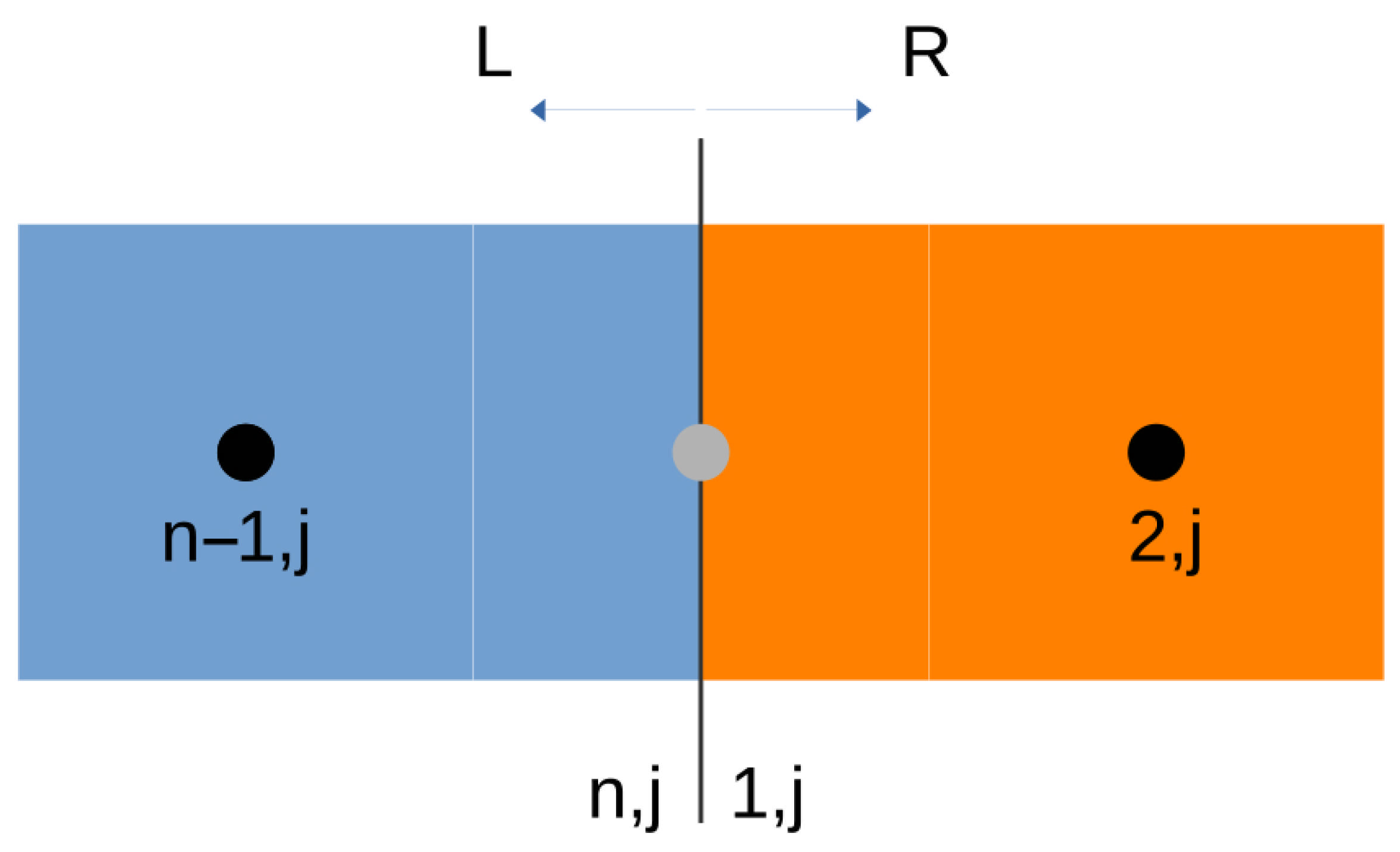
The approach employed in this study is a generalization for curvilinear coordinates, based on previous work detailed in the article [25]. To illustrate this concept, consider a scenario where the interface is normal to the ξ coordinate direction for both domains. The left region is denoted by the prefix L, while the right region is denoted by R as shown in Figure 2.
In the provided figure, the control point shaded in grey is common to both regions. For the left side, it serves as the final node in the ξ direction of the array, marking the beginning of the orange region. It is essential for the variable at this node to hold the same value for both domains.
In this study, we opt to employ the same approach used in previous works to determine the average value on either side of the interface
U ¯ n , j L = η j 1 2 η j + 1 2 ξ i 1 2 ξ i U ( ξ , η , t ) d ξ d η U ¯ 1 , j R = η j 1 2 η j + 1 2 ξ i ξ i + 1 2 U ( ξ , η , t ) d ξ d η .
Then, the same steps implemented in Section 2.2 must be carried out. When developing, it is important to consider that when the interface corresponds to the first or last node of the element in a specific direction, the variable’s slope is zero. As a result, the scheme’s order is locally reduced at the edges.
We arrive at a semi-discrete expression for the variables on both sides of the interface. In the case of the right side, it results in
d U ¯ R d t = F i + 1 2 , j R V i , j R G i , j + 1 2 R G i , j + 1 2 R V i , j R + S i , j , V i , j R = Δ ξ 2 Δ η h ξ ( η i + 1 4 , j ) h η ( η i + 1 4 , j ) , i = 1
F i + 1 2 , j R = Δ η h η ξ i + 1 2 , η j a i + 1 2 , j + a i + 1 2 , j a i + 1 2 , j + F U i + 1 2 , j + a i + 1 2 , j F U i + 1 2 , j + + a i + 1 2 , j + a i + 1 2 , j U i + 1 2 , j U i + 1 2 , j + G i , j + 1 2 R = Δ ξ h ξ ξ i + 1 4 , η j + 1 2 2 b i , j + 1 2 + b i , j + 1 2 b i , j + 1 2 + G U i , j + 1 2 b i , j + 1 2 G U i , j + 1 2 + b i , j + 1 2 b i , j + 1 2 + U i , j + 1 2 U i , j + 1 2 + .
while the left-side results in
d U ¯ L d t = F i 1 2 , j L V i , j L G i , j + 1 2 L G i , j + 1 2 L V i , j L + S i , j , V i , j L = Δ ξ 2 Δ η h ξ ( η i 1 4 , j ) h η ( η i 1 4 , j ) , i = n
F i 1 2 , j L = Δ η h η ξ i 1 2 , η j a i 1 2 , j + a i 1 2 , j a i 1 2 , j + F U i 1 2 , j a i 1 2 , j F U i 1 2 , j + a i 1 2 , j + a i 1 2 , j U i 1 2 , j U i 1 2 , j + G i , j + 1 2 R = Δ ξ h ξ ξ i 1 4 , η j + 1 2 2 b i , j + 1 2 + b i , j + 1 2 b i , j + 1 2 + G U i , j + 1 2 b i , j + 1 2 G U i , j + 1 2 + b i , j + 1 2 b i , j + 1 2 + U i , j + 1 2 U i , j + 1 2 + .
Using the numerical integrator, we determine the variables for the next time. The value in the interface will be the average of these variables:
U i , j = V i , j L u i , j L + V i , j R u i , j R V i , j R + V i , j L .
This process also applies if the interface is oriented in the η direction. Other situations may arise where in one domain it is in the η direction and in the other it is in the ξ direction. The developed software encompasses all possible interactions.

3. Numerical Tests

In this section, we conduct a study of the external flow over bodies by employing the method outlined in the previous section. The codes for the implementation were developed by the authors using the Julia programming language.
To handle the boundary conditions, we utilize two types: Dirichlet, where the variable value is defined, and Neumann, where the zero gradient is defined.
The initial two tests, involving flow over a cylinder and flow over a blunt body, were conducted to validate our software and the numerical techniques we have implemented. The third test, which involves flow over a wedge, includes interfaces between different zones within the physical domain and utilizes the new methodology introduced in this study.

3.1. Flow over a Cylinder

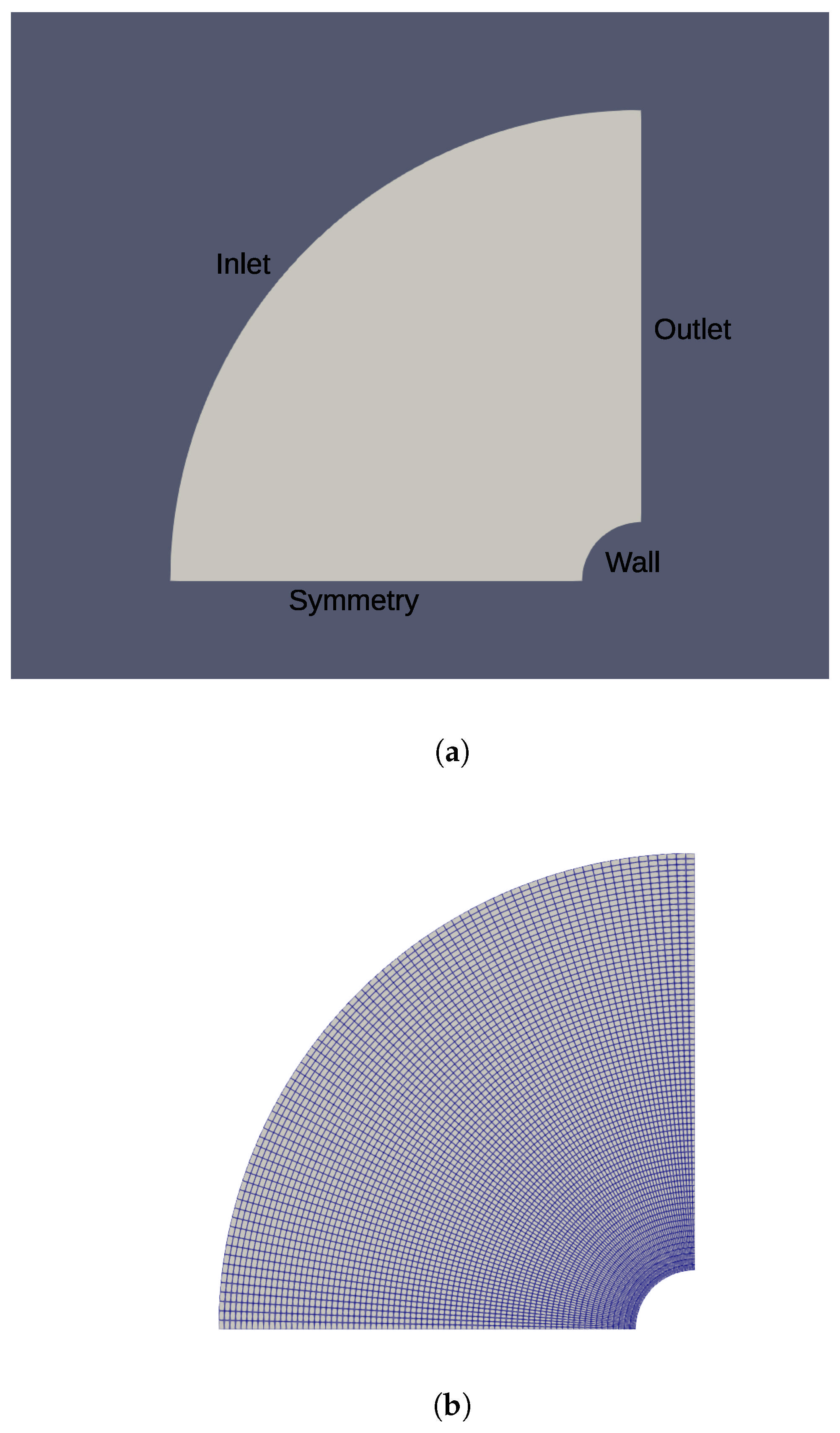
The analysis is confined to two-dimensional cases. Therefore, the flow around a circle is studied. Due to the dual symmetry of the issue at hand, we consider only a quarter of the domain as illustrated in Figure 3a. Figure 3b shows the used mesh of 40,000 elements or cells.
In this test, as it is a single region, there is no interface to consider. The coordinates used for the domain are polar, with ξ = r and η = θ .
In this assessment, the test is performed under ambient conditions characterized by p = 101,325 Pa and T = 298 K. The inlet velocity is oriented horizontally and has a Mach number of 2 ( M = 2 ). It is crucial to emphasize that the velocity is expressed in Cartesian coordinates, necessitating its conversion and evaluation in the corresponding polar coordinates.
The implemented boundary conditions for this test are described in Table 1.
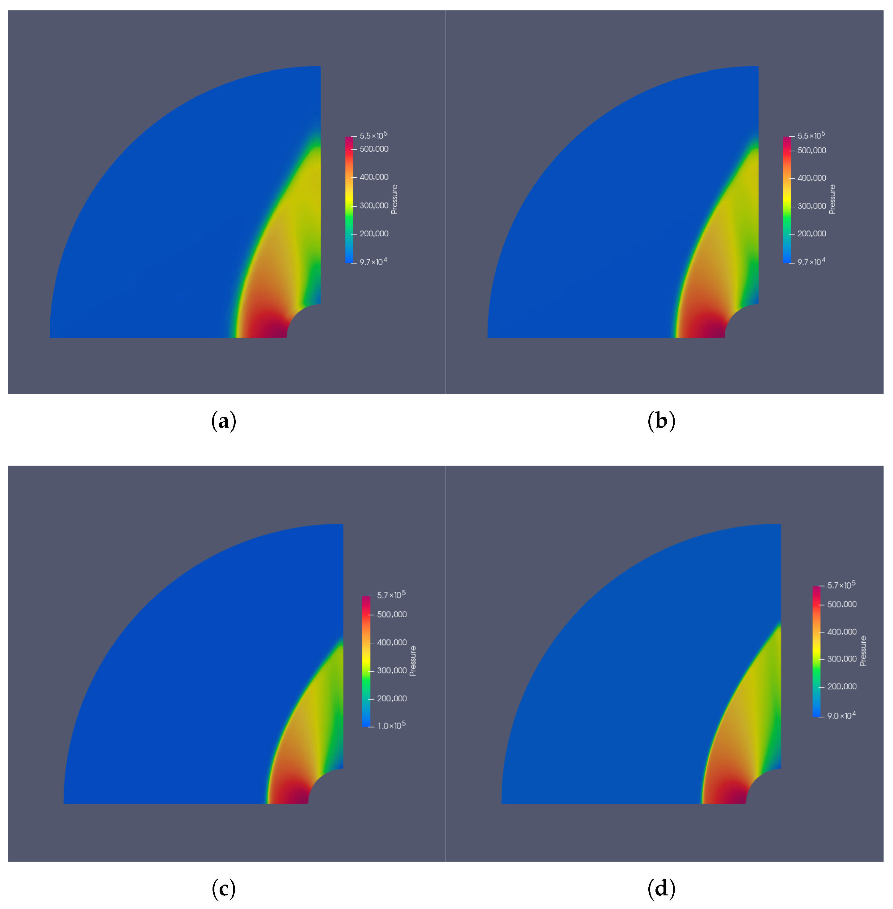
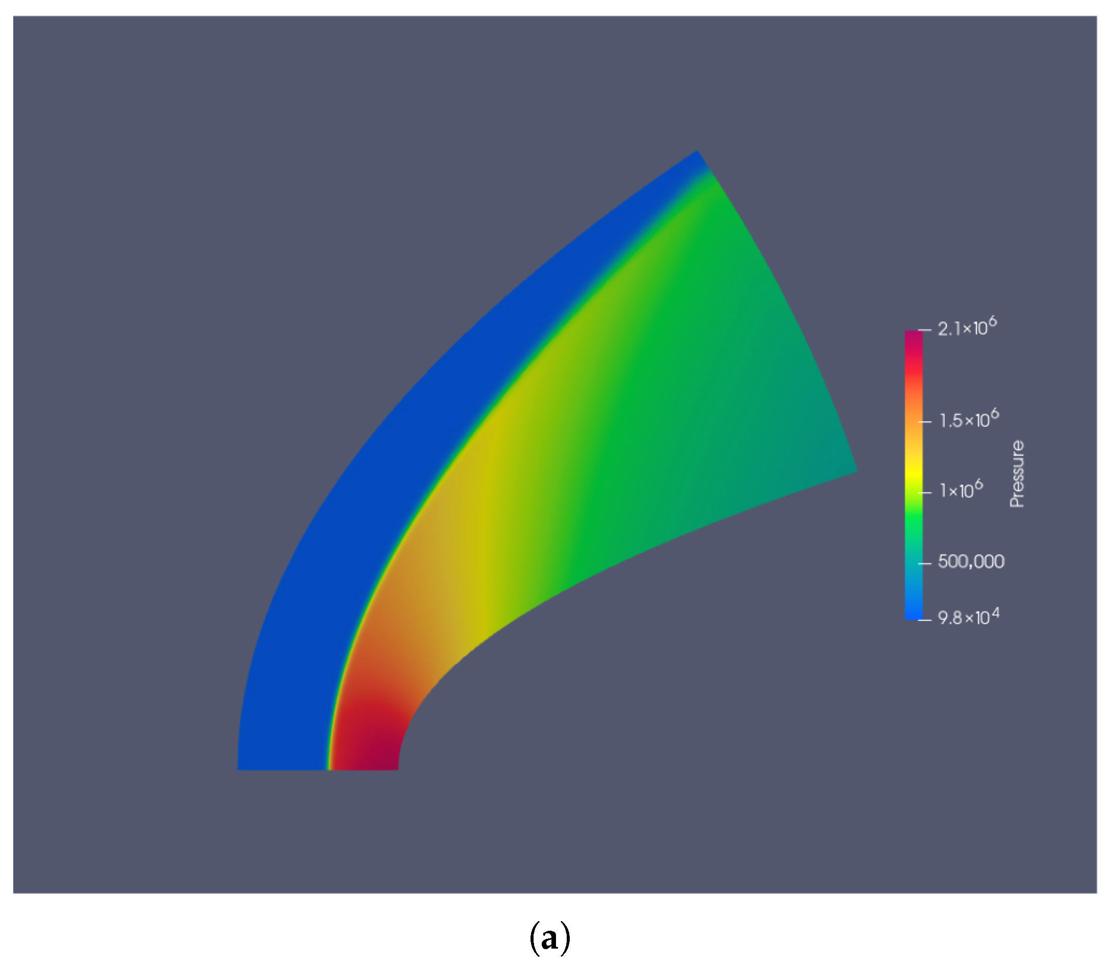
We perform multiple simulations using meshes with varying numbers of cells. Figure 4 illustrates the pressure field acquired in each simulation.
At the symmetry axis y = 0 , the shock wave can be studied as a normal shock. Consequently, we can apply the normal shock wave relations in this specific zone [2]. For the current test, with a Mach number of 2, the ratio of stagnation pressure after shock to static inlet pressure is p 0 p = 5.6403 . Table 2 displays the percentage error of the method’s result compared to p 0 p .

3.2. Flow over a Blunt Body

This case involves the analysis of the supersonic external flow over a blunt body, represented by a parabolic cylinder. The equation defining the parabola is as follows:
x = 0.769 y 2 1
Given the geometry, a single domain is used while working in parabolic coordinates. The relationship between parabolic and Cartesian coordinates is
x = 1 2 ξ 2 η 2 0.6749 , y = ξ η , h ξ = h η = ξ 2 + η 2
Note that if we use η = 0.80635 in Equation (47), we recover Equation (46).
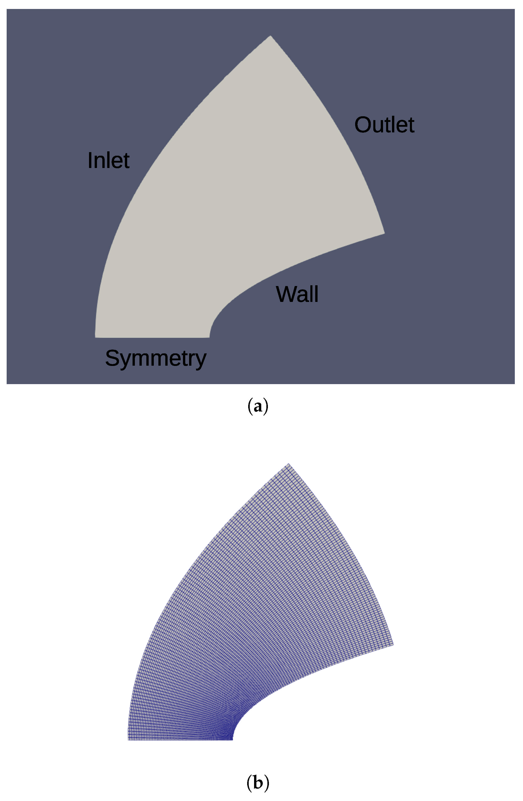
Figure 5a illustrates the physical domain and boundary conditions, while Figure 5b shows the mesh consisting of 102,400 elements. In addition, Table 3 describes the implemented boundary conditions.
Again, we consider the following ambient conditions: p = 101,325 Pa, T = 298 K, and an external velocity with a Mach number equal to two ( M = 2 ) specified in terms of the Cartesian coordinates x.
The present test is similar to the cylinder, as normal shock wave relations apply when analyzing the axis where y = 0 . Thus, according to [2], the relationship is expressed as p 0 / p = 21.0698 , where p 0 is the stagnation pressure after the shock wave.
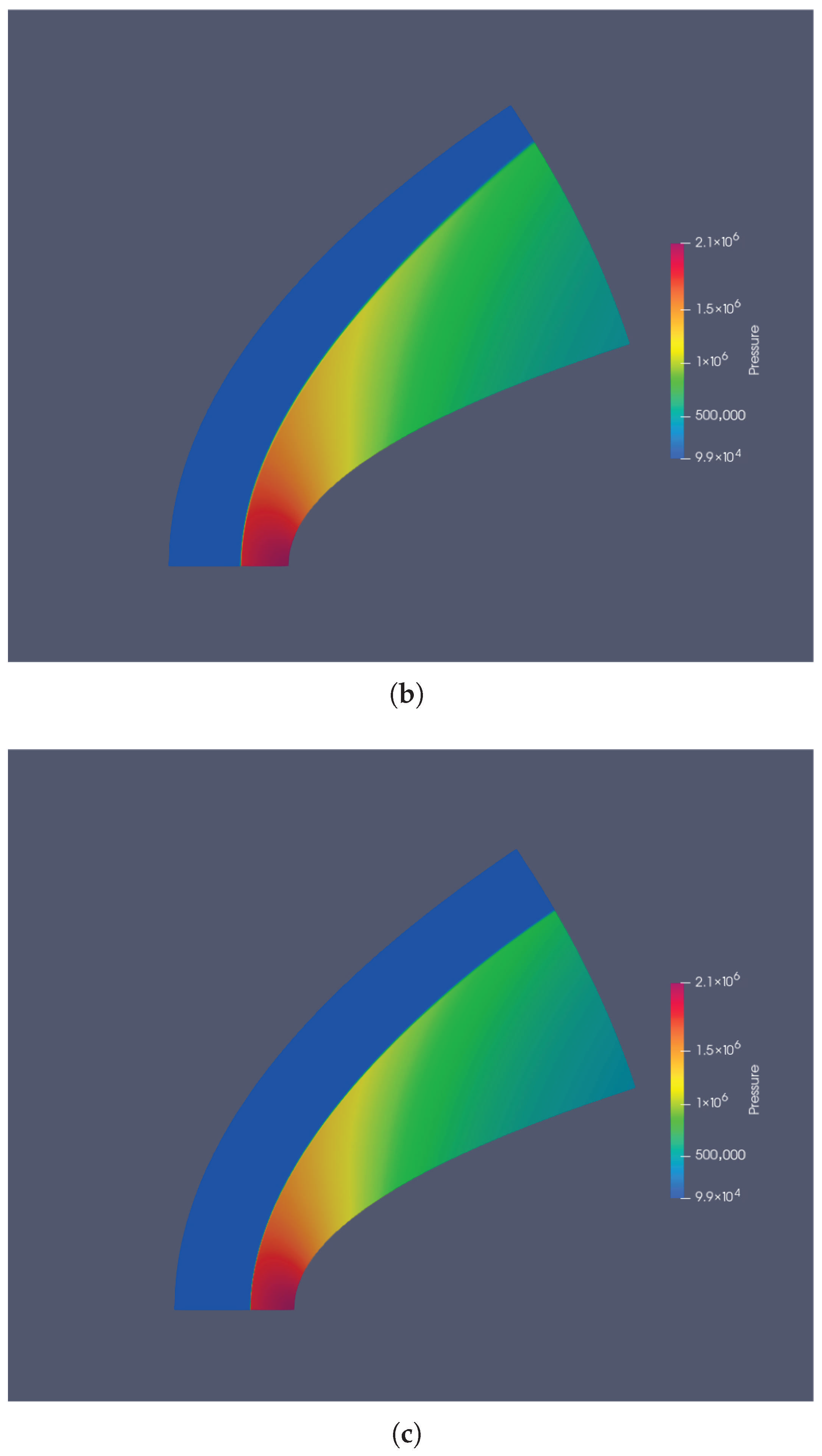
Note that for a coarse mesh, the error is less than 5 % . Furthermore, for a dense mesh, the error reduces to less than 1 % .
Figure 6 displays the resulting pressure distribution for meshes with different numbers of cells. Table 4 presents the percentage error of p 0 / p for various meshes.

3.3. Flow over a Wedge

We analyze the flow around a wedge. Due to the domain’s symmetry, we simulate only half of it. The exact steady-state solution of this problem is presented in [2].
This test comprises three subdomains and two interfaces as shown in Figure 7a. Additionally, Table 5 presents the boundary conditions for each subdomain, and Figure 7b depicts the implemented mesh (26,400 cells).
The external ambient conditions are as follows: the static pressure is p = 101,325 Pa, the static temperature is T = 298 K, and the Mach number is M = 2 in the horizontal direction.
Based on [2], for the current case with supersonic flow over a wedge, the static pressure ratio before and after the shock wave is p 2 / p = 2.82 . This pressure relation was confirmed for all developed simulations. The angle formed by the shock wave with the horizontal axis is also crucial, and it should be β = 32 . 24 ° . Using the numerical scheme with 30,000 cells, an angle of β = 32 . 07 ° was obtained, resulting in a 0.5 % error. Figure 8 shows the numerical results.
Table 2 displays the error in the shock wave angle for five meshes. We can note how the numerical solutions approach the analytical one as the mesh becomes increasingly dense.
From Figure 4, Figure 6, and Figure 8, we can observe that the numerical diffusion introduced by the new scheme to capture the shock waves decreases as the mesh becomes denser. This is evidenced by the reduction in the area experiencing pressure changes around the shock waves. In addition, the numerical diffusion introduced by the new method is less than that generated by OpenFOAM using the KNP scheme.
To calculate the order of the scheme, we use the following equation [26,27]:
s i j = log | u j u i | | u j + 1 u j | log ( N j / N i )
where s i j is the method’s order, u i and N i are the numerical solution and the number of elements of the mesh i, respectively. The numerical value under consideration is the angle of the shock wave.
We apply Equation (48) to the values in Table 6 and find s 12 = 0.045 , s 23 = 1.81 , and s 34 = 2.1 . Therefore, the new scheme converges to second-order accuracy.
We would like to emphasize that the angle of the shock wave calculated by OpenFOAM using a mesh of 30,000 elements is 32 . 84 ° . In contrast, the angle determined by our newly introduced method is 32 . 07 ° , while the analytical value for the shock wave angle is 32 . 24 ° . These results indicate that the new scheme effectively and accurately evaluates the phenomenon under investigation.

4. Conclusions

In this research, we extend the Kurganov–Tadmor scheme for solving Euler equations in two-dimensional curvilinear coordinates.
To determine the average vector of conservative variables, denoted as U ¯ , we first divide the cell into eight sub-cells. Each sub-cell’s average is influenced by the neighboring cells, and we assess these influences. Subsequently, we apply Equation (21) to compute U ¯ for the entire cell, ensuring an accurate representation of the average across the complete structure. This method accounts for spatial interactions and enhances the reliability of our calculated averages. We employ a fourth-order Runge–Kutta temporal integrator and incorporate an interface treatment to handle several mesh types. This scheme can manage interfaces across different regions of the physical domain.
To validate its performance, we test the scheme on three different cases: supersonic flow over a cylinder, a blunt body, and a wedge. For the three tests, the numerical results are promising, indicating that this method is a feasible approach for simulating flow around various objects. Its ability to handle different coordinate systems within the same domain, connected through the interface treatment, demonstrates excellent convergence as the mesh resolution increases.
We note that implementing meshes with different topologies can restrict the time step, thus increasing the total CPU time of the simulation.
The proposed method is especially beneficial for analyzing a variety of external flows over objects. It allows the division of the domain into independent zones, each with its coordinate system. These zones are interconnected through the interface treatment previously described.
The new method achieves second-order accuracy and provides more precise results than the classical Kurganov–Tadmor–Petrova scheme when both methods use similar meshes. This improvement underscores its potential as a valuable tool for enhancing computational precision.
The study presented herein represents a preliminary step in the development of a novel numerical scheme. Subsequent research will be essential in assessing its potential.

Author Contributions

Conceptualization, S.B. and S.E.; methodology, S.B.; software, S.B.; validation, S.B. and L.G.M.; formal analysis, S.B. and S.E.; investigation, S.B., S.E. and L.G.M.; resources, S.B. and S.E.; data curation, S.B. and L.G.M.; writing—original draft preparation, S.B., S.E. and L.G.M.; writing—review and editing, S.B., S.E. and L.G.M.; visualization, S.B. and L.G.M.; supervision, S.E.; project administration, S.E.; funding acquisition, S.E. All authors have read and agreed to the published version of the manuscript.

Funding

This research was funded by the Project 33620180100218CB, Secretary of Science and Technology of the National University of Córdoba, and PIP-2021-2023-GI-11220200101463CO of CONICET.

Data Availability Statement

The authors will be able to provide data and tools upon reasonable request.

Acknowledgments

The authors would like to thank José Tamagno for their teachings.

Conflicts of Interest

The authors declare no conflicts of interest.

References

  1. Anderson, J. Hypersonic and High Temperature Gas Dynamics; McGraw-Hill: Boston, MA, USA, 1989. [Google Scholar]
  2. Anderson, J. Modern Compressible Flow: With Historical Perspective, 3rd ed.; McGraw-Hill: Boston, MA, USA, 2003. [Google Scholar]
  3. LeVeque, R. Finite Volume Methods for Hyperbolic Problems, 1st ed.; Cambridge University Press: Cambridge, UK, 2004. [Google Scholar]
  4. Bakhtiyarov, S.; Adanur, S. Airflow over Wavy Yarn in Air-Jet Filling Insertion. Math. Comput. Appl. 1999, 4, 1–7. [Google Scholar] [CrossRef]
  5. Wang, B.; Garg, N. Third-order numerical scheme for Euler equations of gas dynamics using Jordan canonical based splitting flux. Comput. Fluids 2024, 281, 106370. [Google Scholar] [CrossRef]
  6. Trojak, W.; Dzanic, T. Positivity-preserving discontinuous spectral element methods for compressible multispecies flows. Comput. Fluids 2024, 280, 106343. [Google Scholar] [CrossRef]
  7. Tamagno, J.; Elaskar, S.; Ríos, G. Numerical simulation of time-dependent reacting flows in pulse facilities. Appl. Numer. Math. 2003, 47, 515–530. [Google Scholar] [CrossRef]
  8. Falcinelli, O.; Elaskar, S.; Tamagno, J. Reducing the numerical viscosity in non-structured three-dimensional finite volumes computations. J. Spacecr. Rocket AIAA 2008, 45, 406–408. [Google Scholar] [CrossRef]
  9. Toro, E. Riemann Solvers and Numerical Methods for Fluid Dynamics, 3rd ed.; Springer: Berlin, Germany, 2009. [Google Scholar]
  10. EsfandAbadi, M.; Mohammadi, A.; Djavareshkian, M. Design and analysis of supersonic inlet for ramjet engines: Aerodynamic considerations and performance optimization. J. Aerosp. Sci. Technol. 2024, 17, 47–59. [Google Scholar]
  11. Araya, G. Unsteady subsonic/supersonic flow simulations in 3D unstructured grids over an acoustic cavity. Fluids 2024, 9, 92. [Google Scholar] [CrossRef]
  12. Kurganov, A.; Noelle, S.; Petrova, G. Semidiscrete central-upwind schemes for hyperbolic conservation laws and hamilton-jacobi equations. J. Sci. Comput. 2001, 23, 707–740. [Google Scholar] [CrossRef]
  13. Kurganov, A.; Tadmor, E. New high-resolution central schemes for nonlinear conservation laws and convection–diffusion equations. J. Comput. Phys. 2000, 160, 241–282. [Google Scholar] [CrossRef]
  14. Illenseer, T.; Duschl, W. Two-dimensional central-upwind schemes for curvilinear grids and application to gas dynamics with angular momentum. Comput. Phys. Commun. 2009, 180, 2283–2302. [Google Scholar] [CrossRef]
  15. Greenshields, C.; Weller, H.; Gasparini, L.; Reese, J. Implementation of semi-discrete, non-staggered central schemes in a colocated, polyhedral, finite volume framework, for high-speed viscous flows. Int. J. Numer. Math. Fluids 2010, 63, 1–21. [Google Scholar] [CrossRef]
  16. Gutiérrez Marcantoni, L.; Tamagno, J.; Elaskar, S. rhocentralrffoam: An openfoam solver for high speed chemically active flows—Simulation of planar detonations. Comput. Phys. Commun. 2017, 219, 209–222. [Google Scholar] [CrossRef]
  17. Gutiérrez Marcantoni, L.; Tamagno, J.; Elaskar, S. Numerical study on the impact of chemical modeling on simulating methane-air detonations. Fuel 2019, 240, 289–298. [Google Scholar] [CrossRef]
  18. Weng, Z.; Mével, R. Implementation of an openfoam solver for shock and detonation simulation at high pressure. Comput. Fluids 2023, 265, 10601. [Google Scholar] [CrossRef]
  19. Kreiss, H.; Ortiz, O. Introduction to Numerical Methods for Time Dependent Differential Equations; Wiley: Hoboken, NJ, USA, 2014. [Google Scholar]
  20. Landau, L.; Lifshitz, E. Mecánica de Fluidos, Vol, 6, Colección de Física Teórica; Reverté: Barcelona, Spain, 1986. [Google Scholar]
  21. Whitham, G. Linear and Nonlinear Waves; John Wiley & Sons: New York, NY, USA, 1974. [Google Scholar]
  22. Aris, R. Vectors, Tensors, and the Basic Equations of Fluid Mechanics; Dover Publications: Mineola, NY, USA, 1989. [Google Scholar]
  23. Tannehill, J.; Anderson, D.; Pletcher, R. Computational Fluid Mechanics and Heat Transfer, 2nd ed.; Taylor & Francis: Washington, DC, USA, 1997. [Google Scholar]
  24. Chapra, S.; Canale, R. Numerical Methods for Engineers, 7th ed.; McGraw-Hill Education: New York, NY, USA, 2015. [Google Scholar]
  25. Montes, P.; Reula, O. New numerical interface scheme for the Kurganov-Tadmor second-order method. arXiv 2021, arXiv:2105.03452. [Google Scholar]
  26. Roache, P. Verification and Validation in Computational Science and Engineering; Hermosa: Albuquerque, NM, USA, 1998. [Google Scholar]
  27. Oberkampf, W.; Trucano, T. Verification and validation in computational fluid dynamics. Prog. Aerosp. Sci. 2002, 38, 209–272. [Google Scholar] [CrossRef]
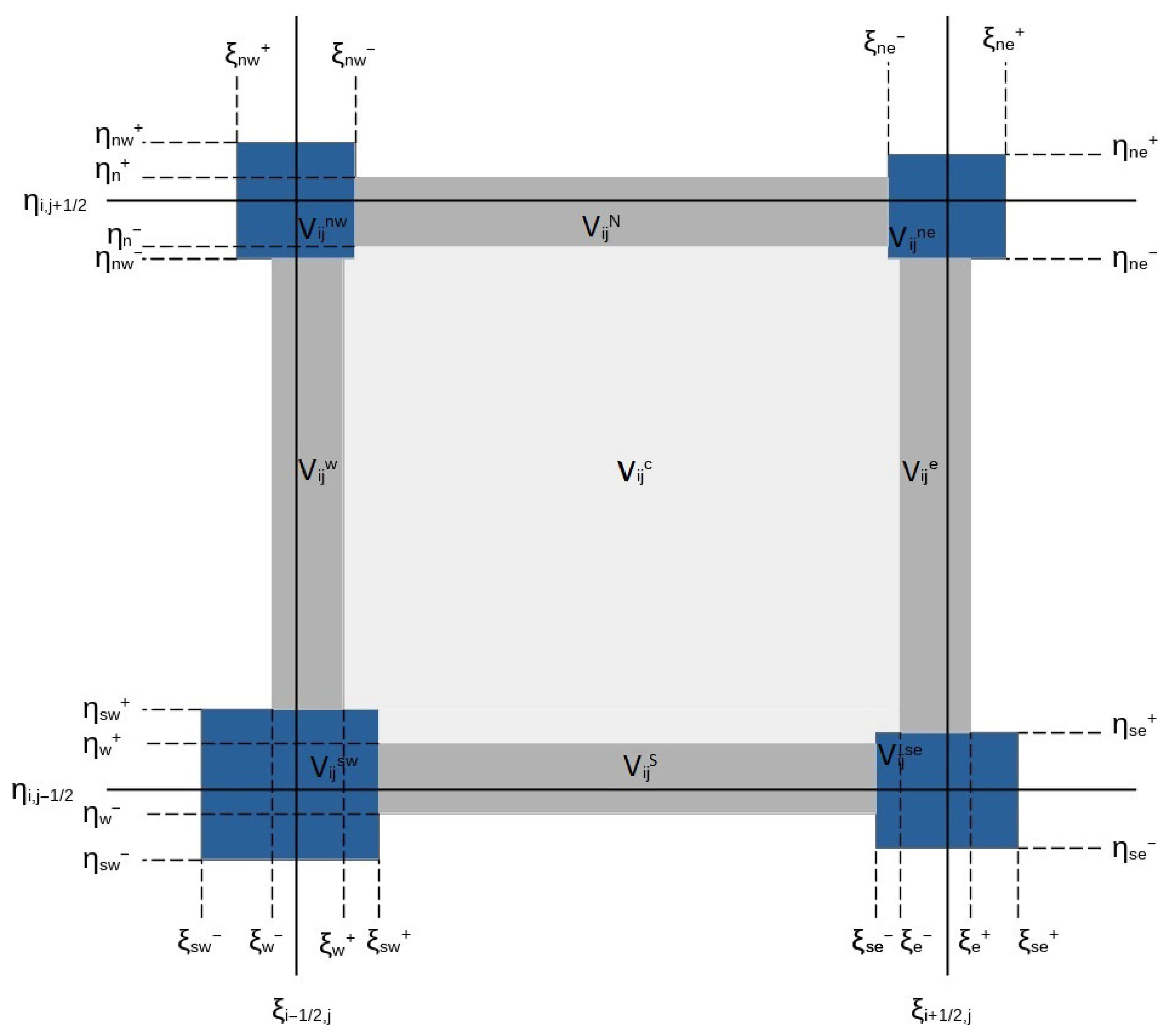
Figure 1. Cell’s sub-division.
Mca 30 00092 g001
Figure 2. Regions interface.
Mca 30 00092 g002
Figure 3. Flow over a cylinder. (a) Domain and boundary conditions. (b) Mesh.
Mca 30 00092 g003
Figure 4. Cylinder: pressure distribution for different numbers of cells, t = 0.3 s: (a) 2700 cells, (b) 6000 cells, and (c) 14,000 cells. (d) 40,000 cells.
Mca 30 00092 g004
Figure 5. Flow over a blunt body. (a) Domain and boundary conditions. (b) Mesh.
Mca 30 00092 g005
Figure 6. Blunt body: pressure distribution for different numbers of elements, t = 0.1 s: (a) 8100 cells, (b) 44,200 cells, and (c) 102,400 cells.
Mca 30 00092 g006aMca 30 00092 g006b
Figure 7. Flow over a wedge. (a) Domain and boundary conditions, (b) Mesh.
Mca 30 00092 g007
Figure 8. Edge: pressure distribution for different numbers of elements, t = 0.8 s: (a) 10,400 cells, (b) 13,000 cells, and (c) 26,400 cells.
Mca 30 00092 g008
Table 1. Boundary conditions for the cylinder test.
uvpT
  InletDirichlet
u ξ = u ξ a m b
Dirichlet
u η = v ξ a m b
Dirichlet
p = p a m b
Dirichlet
T = T a m b
  OutletDirichlet
u ξ = 0
  Neumann  Neumann  Neumann
  Symmetry  NeumannDirichlet
u η = 0
  Neumann  Neumann
  WallDirichlet
u ξ = 0
  Neumann  Neumann  Neumann
Table 2. Errors in cylinder simulation.
Number of Cells p 0 / p % Error
27005.39244.39
60005.43453.65
14,4005.5805–5.49031.06–2.659
40,0005.59530.79
Table 3. Boundary conditions for the blunt body test.
uvpT
  InletDirichlet
u ξ = u ξ a m b
Dirichlet
v ξ = v ξ a m b
Dirichlet
p = p a m b
Dirichlet
T = T a m b
OutletNeumannNeumannNeumannNeumann
  SymmetryDirichlet
u ξ = 0
  Neumann  Neumann  Neumann
  Wall  NeumannDirichlet
u η = 0
  Neumann  Neumann
Table 4. Errors in blunt body simulation.
Numbers of Elements p 0 / p % Error
810020.24563.912
44,10020.56662.38
102,00020.94450.595
Table 5. Boundary conditions for the edge’s test.
Subdomain 1
uvpT
  InletDirichlet
u ξ = u ξ a m b
Dirichlet
v ξ = v ξ a m b
Dirichlet
p = p a m b
Dirichlet
T = T a m b
Outletinterfaceinterfaceinterfaceinterface
  Symmetry  NeumannDirichlet
u η = 0
  Neumann  Neumann
PointNeumannNeumannNeumannNeumann
Subdomain 2
uvpT
Leftinterfaceinterfaceinterfaceinterface
Rightinterfaceinterfaceinterfaceinterface
TopNeumannNeumannNeumannNeumann
  Wall  NeumannDirichlet
u η = 0
  Neumann  Neumann
Subdomain 3
uvpT
Inletinterfaceinterfaceinterfaceinterface
OutletNeumannNeumannNeumannNeumann
TopNeumannNeumannNeumannNeumann
PointNeumannNeumannNeumannNeumann
Table 6. Errors in wedge simulation. The columns represent the mesh number, the number of elements in the mesh, the numerical solution for the shock wave angle, and the percentage error relative to the analytical solution.
MeshNumber of CellsShock Wave Angle% Error
13750 31 . 47 ° 2.39
210,400 31 . 69 ° 1.7
313,000 31 . 90 ° 1.05
426,400 32 . 04 ° 0.62
530,000 32 . 07 ° 0.52
Disclaimer/Publisher’s Note: The statements, opinions and data contained in all publications are solely those of the individual author(s) and contributor(s) and not of MDPI and/or the editor(s). MDPI and/or the editor(s) disclaim responsibility for any injury to people or property resulting from any ideas, methods, instructions or products referred to in the content.