Testing Neural Architecture Search Efficient Evaluation Methods in DeepGA

Abstract

Neural Architecture search (NAS) aims to automate the design process of Deep Neural Networks, reducing the Deep Learning (DL) expertise required and avoiding a trial-and-error process. Nonetheless, one of the main drawbacks of NAS is the high consumption of computational resources. Consequently, efficient evaluation methods (EEMs) to assess the quality of candidate architectures are an open research problem. This work tests various EEMs in the Deep Genetic Algorithm (DeepGA), including early stopping, population memory, and training-free proxies. The Fashion MNIST, CIFAR-10, and CIFAR-100 datasets were used for experimentation. The results show that population memory has a valuable impact on avoiding repeated evaluations. Additionally, early stopping achieved competitive performance while significantly reducing the computational cost of the search process. The training-free configurations using the Logsynflow and Linear Regions proxies, as well as a combination of both, were only partially competitive but dramatically reduced the search time. Finally, a comparison of the architectures and hyperparameters obtained with the different algorithm configurations is presented. The training-free search processes resulted in deeper architectures with more fully connected layers and skip connections than the ones obtained with accuracy-guided search configurations.

1. Introduction

Convolutional Neural Networks (CNNs) are one of the most popular and successful Deep Learning (DL) models for image processing. Their basic structure comprises convolutional, pooling, and fully connected layers, which enable the network to automatically extract features from the input data [1]. CNNs have been applied in various computer vision applications, such as image classification, object detection, and image segmentation. Nonetheless, their design requires selecting various network hyperparameters, which influence performance. In addition, no combination of them is guaranteed to provide a competitive configuration in all cases [2,3]. Therefore, manually designing CNNs requires DL experience, knowledge, and a considerable amount of computational resources in specialized hardware like Graphics Processing Units (GPUs) [4,5].

Neural Architecture Search (NAS) provides an alternative to the aforementioned problem by automating the design of the network and its hyperparameter configuration. This way, less domain expertise is required, and the by-hand trial-and-error design process is avoided [6]. As exposed in [7,8], NAS can be divided into three stages: the search space, the search strategy, and the performance estimation method. The search space is determined by the selected encoding mechanism for the network architectures [9]. The search strategy is how the search space is explored. In this case, Evolutionary Computation (EC) algorithms, as population-based meta-heuristics, are a promising approach to guide the search, giving place to the field of Evolutionary Neural Architecture Search (ENAS) [10]. Finally, an efficient way to estimate the performance of a candidate architecture is an open problem, given that its training and testing process is costly [11]. A situation that accumulates and demands more resources as several candidate architectures are explored during the search.

A series of efforts to reduce the computational burden of NAS, one of its main disadvantages, is shown in [12]. Four categories of efficient evaluation methods (EEMs) are proposed: N-shot, few-shot, one-shot, and zero-shot. In N-shot methods, the number of architectures explored during the search and the number of trained architectures are the same; however, a strategy is employed to lighten the evaluations. The previous is also known as low-fidelity evaluations. Examples include using low-resolution images or a subset of the training set, and early stopping, which reduces the number of training epochs [4,13]. As presented in [14], training an architecture for a few epochs allows for identifying its performance tendency, which is enough to conduct the search process.

Few-shot EEMs follow a scheme where not all architectures examined in the search are trained. Surrogate models are included in this category [15]. An alternative useful for ENAS is population memory, where the encoding and fitness of an architecture are stored in memory. This way, if the search process finds an architecture that has been previously evaluated, the fitness is retrieved from memory, avoiding repeated evaluations [6]. In [16], population memory is included in a Genetic Algorithm (GA) for NAS in image classification. Population memory is also known as a cache for the search process.

One-shot EEMs perform a single training process and are based on transfer learning. Usually, a super-net is trained, and the candidate architectures are sampled from it using weight-sharing mechanisms [11]. Finally, in zero-shot EEMs, no architecture is trained throughout the search process. Instead, training-free score functions rank the architectures [17]. A training-free proxy is usually designed based on a theoretical analysis of Deep Neural Networks (DNNs). The proxies can be classified into two categories: gradient-based and gradient-free [18]. A gradient-based proxy, such as the logarithm of the synaptic flow (Logsynflow) [19], considers the network’s weights and gradient to estimate the network’s trainability. While proxies such as Linear Regions [20] and noise immunity [21] consider activation patterns in the network for scoring, they are deemed gradient-free.

One of the advantages of NAS is that multiple design criteria can be considered to guide the search. For example, the user can define that the search process will not only be guided by the accuracy performance of the architecture but also consider the complexity, prioritizing a model with decent performance and a reduced number of parameters. ENAS leverages the capabilities of EC algorithms to conduct single- and multi-objective optimization processes [7].

The previous is also considered in zero-shot EEMs, where more than one proxy is used during the search. Some approaches combine proxies into a single function to conduct a single-objective optimization process, while others adopt a multi-objective process. Examples of the former include a linear combination of Logsynflow, Linear Regions, and skipped layers in [19], as well as Linear Regions and noise immunity in [22]. A linear combination of proxies introduces an additional complication due to the requirement of normalizing the scores to adjust their ranges. An alternative is presented in [23] with a ranking-based method considering noise immunity, Linear Regions, and Logsynflow. Multi-objective approaches are presented in [24], where synaptic flow is considered in conjunction with the network’s complexity, and [25], where different proxies are tested and combined for comparison with training-based metrics to guide the search.

One of the main drawbacks of training-free proxies is presented in [18], where a series of tested proxies derived in low correlation with test accuracy. Consequently, highly accurate architectures can be discarded in favor of low-performing ones. Most training-free NAS proposals are evaluated in benchmarks like NAS-bench-101 [26], where a cell-based encoding is used, and limited network operations are considered for the search. In addition, a few zero-shot EEM-based works incorporate complexity limitations into the search process. Examples are presented in [20] where the Linear Regions proxy is tested in an unconstrained and a constrained scenario; in [24,25] where the complexity of the network is used as an objective; and in [27] where latency is considered in a hardware-aware network. In the opposite sense, a maximization of the number of trainable parameters and the number of convolutional layers guides the search in [28].

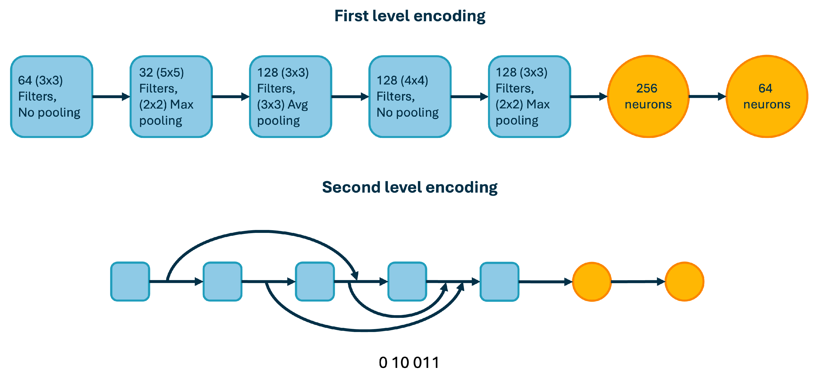
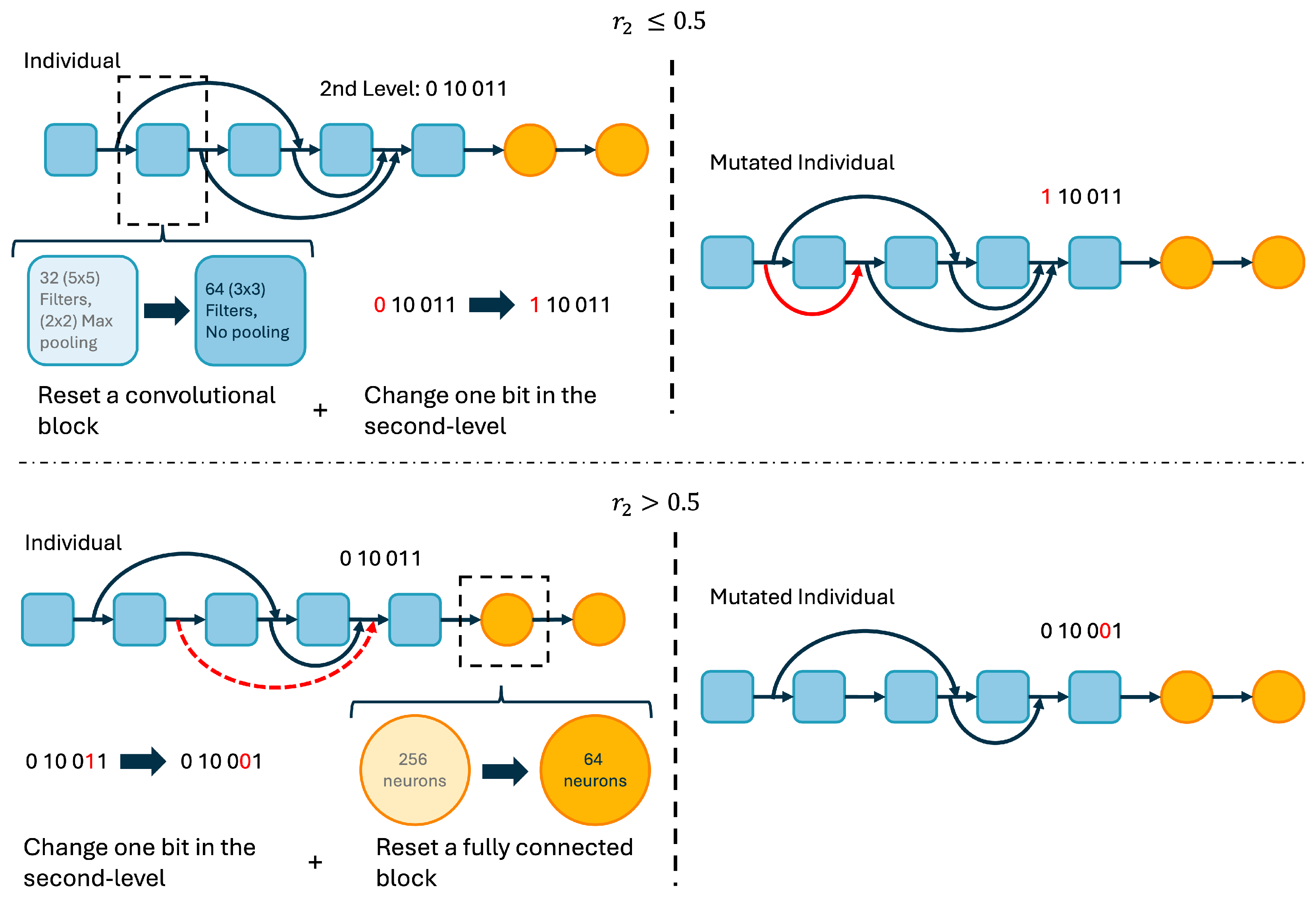
This work extends the research proposal from [29], where cost-reduction mechanisms were applied in the Deep Genetic Algorithm (DeepGA). DeepGA was initially proposed in [30], optimizing the design of CNNs for classifying chest X-ray images to detect COVID-19 and pneumonia cases. The algorithm employs a two-level hybrid encoding considering blocks for the configuration of the network layers at the first level and the skip connections at the second level. One key aspect of the search process is that it is guided by the performance of the network as well as its complexity, measured as the number of trainable parameters. The previous is performed with a weighted combination of both design criteria in the fitness function or through a multi-objective optimization process. DeepGA has also been applied in [31] for breast cancer diagnosis, in [32] for vehicle make and model recognition, in [33] for the estimation of anthocyanins in heterogeneous and homogeneous bean landraces, and in [34] for steering wheel angle estimation.

The EEMs tested in [29] were early stopping, reducing the number of epochs in an evaluation, and population memory to avoid repeated evaluations. The results for the Fashion MNIST dataset [35] indicated that the performance of DeepGA was not diminished, but a significant reduction in running time was achieved. Nonetheless, the results were limited to only one dataset with a reduced number of algorithm runs. In light of the above, the first step of this paper’s research proposal is to extend the experimentation using early stopping and population memory to more challenging datasets and analyze if the findings hold. The CIFAR-10 and CIFAR-100 datasets [36], two benchmark datasets in image classification, are considered in addition to Fashion MNIST for evaluating the cost-reduction mechanisms. Moreover, this paper proposes a zero-shot EEM scheme for DeepGA, aiming to reduce costs further. The proposal is based on implementing the training-free proxies of Logsynflow and Linear Regions, as well as a combination of these, in the weighted fitness function of single-objective DeepGA. The above implies testing the capabilities of the zero-shot EEM approach to guide the search, where network complexity is considered as a design criterion.

The efforts to reduce the computational cost of DeepGA align with the Green Artificial Intelligence trend [37], following a more efficient search process. This way, the search process of future applications using DeepGA to find CNN architectures is lightened, and fewer energy resources are required. The main contributions of the paper are presented next:

• The effects of using the population memory and the early stopping mechanisms (5 and 10 training epochs) in the search process of DeepGA are reported using the Fashion MNIST, CIFAR-10, and CIFAR-100 datasets.
• Two different training-free proxies are used to guide the search process of DeepGA with the consideration of network complexity as design criteria. Two normalization methods are tested to evaluate which one allows a more suitable implementation in the fitness function of DeepGA.
• The resulting architectures from the accuracy-guided and the training-free-based search processes are compared in detail. The performance, complexity, required computational resources, and the resulting network elements and hyperparameters are analyzed to detect trends in the use of cost-reduction mechanisms.

The rest of the paper is divided into five sections. Section 2 provides the NAS foundations. Section 3 details the materials and methods used in this study, describing the DeepGA methods (Section 3.1), exposing the training free proxies considered (Section 3.2), and addressing the data used for experimentation (Section 3.3). In Section 4, the experimental results are displayed, including performance metrics and statistical evidence. Those are later discussed in Section 5, where assessments are derived based on evidence from results. Finally, Section 6 summarizes outcomes and highlights important conclusions and directions for future work.

2. Background of Neural Architecture Search

The mathematical formulation of NAS as an optimization problem is presented in [7]:

$$\left\{\begin{array}{c}{arg\; min}_A=\mathcal{L}(A,{\mathcal{D}}_{train},{\mathcal{D}}_{fitness})\hfill \\ s.t.A\in \Omega \hfill \end{array}\right.$$

(1)

where $\mathcal{L}(·)$ represents the performance of the architecture A after being trained with ${\mathcal{D}}_{train}$ and evaluated using ${\mathcal{D}}_{fitness}$. $\mathcal{L}(·)$ varies depending on the task and the evaluation strategy selected for the NAS procedure. For example, $\mathcal{L}(·)$ can be the accuracy performance in classification, the mean square error in regression, or a training-free proxy with zero-shot EEMs. Finally, $\Omega$ represents the set of all possible architectures, which constitutes the search space and is derived from the selected encoding for the search process.

The encoding can be classified into diverse categories. In [9], the classification of fixed- and variable-length is presented. A fixed-length encoding requires the maximum depth of the architecture to be selected before the search process, which reduces $\Omega$, limiting the exploration capabilities of the algorithm. On the other hand, variable-length encoding does not require defining a network depth, as the NAS search process automates this step. One of the complications of using variable-length encodings is adapting the variation operators for the search to work with candidate architectures of different lengths.

In addition, as presented in [38], the encoding is classified into direct and indirect. A direct encoding represents characteristics of the network that need little or no additional processing when decoding the genotype into the phenotype (going from the encoding to the network construction). On the contrary, with an indirect encoding, a series of transformation rules must be followed to obtain the phenotype. Additionally, a hybrid approach can be employed, combining direct and indirect encoding methods for the networks.

3. Materials and Methods

3.1. DeepGA

DeepGA was proposed in [30] for designing CNNs. A key aspect of the algorithm is controlling the network’s complexity based on the number of parameters it has. The complexity is considered in two ways: as a penalization when the single-objective version is used and as an objective when working with the multi-objective version. The encoding is a hybrid consisting of two levels. The first level includes blocks that directly represent the network’s layers and hyperparameters. The blocks are divided into convolutional blocks and fully connected blocks, according to the type of layer they represent. Convolutional blocks are positioned at the beginning of the network, while fully connected ones are placed at the end. The second level is an indirect encoding using a binary string that codifies the skip connections for the convolutional blocks starting from the third one, which is the first that can receive a skip connection from the first one. Figure 1 presents an example of the encoding used in DeepGA.

In the convolutional blocks, hyperparameters included are the filter size, the number of filters, and whether the pooling operation is conducted at the output of the convolutional layer. In case the block includes pooling, the type (max or average) and the pooling kernel size are determined. Some hyperparameters are fixed, such as the rectified linear unit (ReLU) as the activation function, batch normalization, a stride of 1 for the convolutional layers, and a stride of 2 for pooling. In the fully connected blocks, the only hyperparameter included is the number of neurons; the ReLU activation function is also used. DeepGA employs a specialized procedure when the skip connections require dimensional adjustments. If the output size of the layer where the skip connection originates is larger than the input size of the target layer, max-pooling is used with a stride of 1 and a kernel size calculated as the output size minus the input size plus 1. When the output size where the skip connection starts is smaller than the input size of the end of the connection, zero padding is used to match the dimensions.

Table 1. Hyperparameter options considered for the convolutional and fully connected blocks of DeepGA and the parameters of the GA.

Network Hyperparameters		GA Parameters
Conv. filter size	{2, 3, 4}	N	20
No. of conv filters	{8, 16, 32, 64, 128, 256}	T	40
Pooling type	{Max, Avg, off}	$CR$	0.7
Pooling kernel size	{2, 3}	$MR$	0.5
No. of neurons FC	{16, 32, 64, 128, 256, 512}	$t_s$	5

presents the parameters selected for experimenting with DeepGA. The network hyperparameters were adjusted through trial and error, initially using the CIFAR-10 dataset. The GA parameters include the population size N, the maximum number of generations T, the crossing rate $CR$, the mutation rate $MR$, and the tournament size $t_s$.

DeepGA follows a classic evolutionary process where the population of size N is randomly initialized. Then, for each algorithm generation, $N/2$ parents are selected using a stochastic tournament where $t_s$ individuals of the population are compared, and the best of them is chosen with a probability of 80%. Otherwise, the parent is selected randomly among the $t_s$ individuals. After that, the crossover and mutation operators are applied to generate $N/2$ individuals as offspring. At the end of each generation, the offspring are added to the population, and an elitist replacement is applied to select the best N individuals that will form the next generation population. In the single-objective version of DeepGA, the fitness values are used to sort the individuals. In contrast, the non-dominated sorting procedure from [39] is used in the multi-objective version. The process is repeated until generation T is reached and the best solution found is returned in the single-objective version or the set of non-dominated solutions in the multi-objective version. In this work, the single-objective version of DeepGA is used.

3.1.1. Fitness Function

DeepGA considers the performance and the complexity of the network as design criteria for the search process. This way, the design of the network is also guided towards less complex architectures. DeepGA has two versions: single- and multi-objective. In the single-objective version, the network’s performance, measured as accuracy, and its complexity, measured by the number of trainable parameters, are combined into a single and weighted function, as presented in Equation (2).

$$f\left(A\right)=(1-w)\ast accuracy\left(A\right)+w\ast {\displaystyle \frac{MP-NP}{MP}}$$

(2)

A corresponds to the network architecture that is being evaluated. $MP$ represents a parameter that the user defines according to a maximum number of architecture parameters. $NP$ is the number of parameters of A. Finally, w represents a factor used to weight the design criterion of the network. Larger values of w will make the complexity of the network more important in the fitness calculation and vice versa.

On the other hand, the multi-objective version of DeepGA considers performance and complexity to be two separate objectives. The main difference between the single-objective version and the multi-objective version is that the latter returns a set of solutions representing a trade-off between accuracy and the number of parameters in the network. This way, the user has different architectures from which to choose.

3.1.2. Crossover

In crossover, the genetic information of the selected parents is combined to generate offspring. Two parents are used to create two descendants. Since two levels form the encoding, the crossover operator is applied at both levels. The first level works with the blocks; in this case, m and n are calculated. Considering the parent with fewer convolutional blocks, m corresponds to the floor function of the number of convolutional blocks divided by 2. The calculation of n considers the parent with fewer fully connected blocks, and n is the floor function of half the number of fully connected blocks. The offspring is generated by swapping the parents’ last m convolutional blocks and the last n fully connected blocks.

In the second level, c is calculated as the floor function of half the length of the shortest bit string of the two parents selected to perform the crossover. Then, the last c bits of the second-level encoding are exchanged. Figure 2 presents an example of the crossover procedure in DeepGA. The crossover procedure of the two parents is applied with a crossover rate defined by the user. Otherwise, the offspring is generated by just copying the parents.

3.1.3. Mutation

The mutation operator applies changes to an individual. DeepGA mutation modifies both levels of the encoding. The modifications are applied according to two random numbers, $r_1$ and $r_2$, from a uniform distribution in the range (0, 1). If $r_1\ge 0.5$, one of the blocks is restarted, changing the hyperparameters encoded there. The type of block to be reinitialized is subject to $r_2$. If $r_2\le 0.5$, one of the convolutional blocks is randomly chosen and restarted. Otherwise ($r_2>0.5$), the randomly chosen block to be restarted is one of the fully connected ones. This mutation process is complemented by a bit flip in the second-level encoding, which changes one skip connection. Figure 3 presents an example of the mutation where a block is restarted.

If $r_1<0.5$, a block is added to the encoding. When $r_2\le 0.5$, a convolutional block with a random initialization of its hyperparameters is inserted in a position selected by chance. The addition of a convolutional block requires changes to the second level encoding, where the required bits (randomly selected) are attached to the positions where needed to complete the representation of skip connections. Alternatively, if $r_2>0.5$, the block to be added is a fully connected one. Similarly to the addition of the convolutional block, the fully connected block to be added is randomly initialized, and the position is determined at random. Figure 4 presents an example of applying the mutation, adding a block to the encoding.

3.2. Training-Free Proxies

Given that no architecture is trained during the search process, zero-shot EEMs using training-free score functions can achieve an extreme computational cost reduction in NAS [18]. This work tests two score functions: Logsynflow, as a gradient-based proxy, and Linear Regions, as a gradient-free proxy. The works of [19,23] inspired the selection of these proxies. The rationale behind the choice is to have one of the proxies, the Logsynflow, considering the network’s trainability, and the other, the Linear Regions, evaluating the network’s expressive capacity. In addition, the combination of them will complement each other.

Nonetheless, as presented in [18], the training-free proxies tend to prefer more complex networks. The Linear Regions proxy that considers the expressive capacity finds potential in models with immense width and depth, given their ability to represent almost any complex function with small error. On the other hand, the trainability of the networks, considered by Logsynflow, is also better in wider networks of similar depth. The above considerations highlight the need to constrain the complexity of the networks in the DeepGA search process, incorporating the number of parameters as a design criterion. The integration of the training-free proxies in the fitness function of DeepGA requires the scores to be scaled similarly to the complexity term of the equation. More details of each proxy are provided next, along with two options for normalizing the metric values and incorporating them into DeepGA.

3.2.1. Logsynflow

The calculation of the synaptic flow was proposed in [40] as a technique for network pruning. The calculation of the score (s) is performed using the weight vector $\theta$ and the gradient vector ${\displaystyle \frac{\partial \mathcal{R}}{\partial \theta }}$ as presented in Equation (3). $\mathcal{R}$ represents a scalar loss function calculated with a feedforward pass in the network with parameters $\theta$.

$$s=\theta ·{\displaystyle \frac{\partial \mathcal{R}}{\partial \theta }}$$

(3)

In [19], the method is utilized as a training-free proxy, although some adaptations are made. The calculation of ${\displaystyle \frac{\partial \mathcal{R}}{\partial \theta }}$ is performed with a pass of a matrix of ones with the same shape as a mini-batch of the input to the network, and the gradients are computed with the output going backward. Then, it was proposed to scale the value with a logarithm to avoid gradient explosion as presented in Equation (4). This calculation gives way to the Logsynflow metric. The batch normalization layers are temporarily omitted during Logsynflow calculation to avoid interfering with the gradient flow.

$$s=\theta ·log\left({\displaystyle \frac{\partial \mathcal{R}}{\partial \theta }}+1\right)$$

(4)

3.2.2. Linear Regions

The Linear Regions proxy, also called NAS without training (NASWOT) score or logdet proxy, was proposed in [20] using a binary code to examine the activation patterns in an untrained network with the forward pass of a minibatch ($\mathbf{X}={\left\{x_i\right\}}_{i=1}^M$) of the data. It is based on the ReLU activation function, so it is classified in [17] as a model-dependent score function. Given its nature, ReLU allows the binarization of the activation pattern, distinguishing between active (multiplied by 1) and inactive units (multiplied by 0) and serving as indicator variables. When an input image $x_i$ passes through the network, the indicator variables in the ReLU function form a binary code $c_i$.

The intuition from using $c_i$ is that two inputs with similar binary codes are more challenging for the network to separate, and therefore, they reside in the same linear region. The Hamming distance $d_H(c_i,c_j)$ is used to measure the dissimilarity of the inputs i and j. With this, the kernel matrix ${\mathbf{K}}_H$ is calculated as presented in Equation (5). $N_A$ is the number of ReLU functions considered in the network for the calculation.

$${\mathbf{K}}_H=\left[\begin{array}{ccc}{N}_A-d_H(c_1,c_1)& \dots & N_A-d_H(c_1,c_M)\\ ⋮& \ddots & ⋮\\ N_A-d_H(c_M,c_1)& \dots & N_A-d_H(c_M,c_M)\end{array}\right]$$

(5)

Finally, the score is calculated using the logarithm of the determinant of ${\mathbf{K}}_H$ as presented in Equation (6).

$$s=log{\mathbf{K}}_H$$

(6)

3.2.3. Normalization

The ranges of the training-free proxies do not present an upper bound. This way, they must be normalized to combine them in a fitness function or to correctly apply the complexity term as in the fitness function of DeepGA (Equation (2)). In [19], a max normalization of the scores is performed by dividing the score $s_i$ by the maximum score in the population $s_{max}$ as presented in Equation (7). This normalization form sets a lower bound of 0 and an upper bound of 1 for the solution with the $s_{max}$.

$$s_{norm}={\displaystyle \frac{s_i}{s_{max}}}$$

(7)

An alternative is presented in [22,28] as the z-score normalization. In z-score normalization, the mean ($\mu$) is subtracted from the value and then divided by the standard deviation ($\sigma$) as presented in Equation (8). Nonetheless, the z-score is not guaranteed to be in the range of $[0,1]$; therefore, using a sigmoid function is proposed as shown in Equation (9). The max and z-score normalization are tested during experimentation with the training-free proxies.

$$s_{norm}={\displaystyle \frac{s_i-\mu }{\sigma }}$$

(8)

$$s_{norm}={\displaystyle \frac{1}{1+e^{-\frac{s_i-\mu }{\sigma }}}}$$

(9)

For combining the two training-free proxies into the fitness function of DeepGA, some changes are proposed in Equation (10). $s{1}_{norm}$ represents the calculation and normalization of the Logsynflow score, and $s{2}_{norm}$ refers to the calculation and normalization of the linear region’s score. Using ${\displaystyle \frac{(1-w)}{2}}$ expects an equal contribution of the scores.

$$f\left(A\right)={\displaystyle \frac{(1-w)}{2}}\ast s{1}_{norm}\left(A\right)+{\displaystyle \frac{(1-w)}{2}}\ast s{2}_{norm}\left(A\right)+w\ast {\displaystyle \frac{MP-NP}{MP}}$$

(10)

3.3. Data for Experimentation

Three datasets are used for experimentation: Fashion-MNIST [35], CIFAR-10, and CIFAR-100 [36]. In the three cases, the suggested train/test split of each dataset is considered. Fashion-MNIST consists of 70,000 grayscale images of clothing items, each with a size of 28 × 28 pixels. The data split considers 60,000 images for training and 10,000 test images. The dataset contains ten classes.

CIFAR-10 and CIFAR-100 contain 60,000 color images of 32 × 32 pixels of diverse objects. The datasets were proposed with a suggested partition of 50,000 training images and 10,000 test images. The images in CIFAR-10 are divided into ten balanced classes. This way, the training and test subsets contain 5000 and 1000 images of each class, respectively. CIFAR-100 is similar, but the images are divided into 100 classes. The training and testing subsets contain 500 and 100 images of each class, respectively. As presented in [9], CIFAR-10 and CIFAR-100 are datasets considered benchmarks for evaluating the performance of NAS algorithms.

No data augmentation was considered in this work, as the primary motivation was to test the cost reduction mechanisms. Using additional data during search, especially with accuracy-guided configurations, would require more resources and extend the time necessary to evaluate the architectures. The batch size of 24 used in [30] is kept in the experimentation.

4. Results

The experimentation was divided into two: the accuracy-guided search and the training-free search. The population memory mechanism is used in all the configurations for experimentation. For a fair comparison, the best architecture found in each run is trained for 50 epochs, a configuration proposed in [29]. In the accuracy-guided search, the early stopping mechanism is used in DeepGA to assess the effects on the performance of the resulting architecture and the computational resources required (see Section 4.1). Section 4.2 presents the results of the training-free search. The normalization strategies are first evaluated using the training-free proxies. Then, the Logsynflow and linear region proxies are used independently to guide the search in DeepGA. Finally, a combination of Logsynflow and Linear Regions is used for searching. A comparison among the configurations tested is provided. At the end of this section (Section 4.3), details of the resulting architectures from the different algorithm configurations are compared.

The experimentation consisted of ten runs for each configuration in DeepGA. The value of w was set to 0.1 for the accuracy-guided configurations. The networks were trained using the Adam optimizer with a learning rate of $1\times {10}^{-4}$ and the cross-entropy loss function. The code was executed using Google Colab Pro+ virtual environments with an NVIDIA T4 GPU. The CPU corresponds to a 2.2 GHz Intel Xeon. The code is based on the PyTorch library [41], and the 2.6.0 version was used.

4.1. Accuracy-Guided Search

Two configurations of DeepGA are tested, considering five and ten training epochs, as in [29], to evaluate individuals during the search and analyze the effect of early stopping mechanisms. The performance of both algorithm configurations is presented in

Table 2. Accuracy performance of DeepGA using the accuracy-guided configurations. The best values for each dataset are marked in bold.

Dataset	Configuration	Best	Mean	Std Dev	Worst
Fashion MNIST	Accuracy-10	0.9333	0.9248	0.0045	0.9180
	Accuracy-5	0.9302	0.9256	0.0038	0.9189
CIFAR-10	Accuracy-10	0.8339	0.8145	0.0133	0.7840
	Accuracy-5	0.8542	0.8290	0.0156	0.8094
CIFAR-100	Accuracy-10	0.5566	0.5341	0.0236	0.4938
	Accuracy-5	0.5650	0.5173	0.0288	0.4749

. The tested configurations are identified as Accuracy-10 and Accuracy-5, respectively. The Wilcoxon signed-rank test is performed for pairwise comparison, yielding p-values of 0.7519 for Fashion MNIST, 0.0273 for CIFAR-10, and 0.1930 for CIFAR-100. According to the CIFAR-10 dataset statistics, the configuration with five epochs performed better. Conversely, no significant differences were detected in the methods for the Fashion MNIST and CIFAR-100 datasets. The considerations above show that the early stopping mechanism is capable of maintaining a competitive performance while using fewer training epochs in an evaluation.

Table 3. Average network complexity in terms of trainable parameters and MFLOPS for the accuracy guided configurations of DeepGA. Standard deviation is shown in parentheses.

Dataset	Configuration	No. Parameters	MFLOPS
Fashion MNIST	Accuracy-10	243,438.0 (64,931.6)	140.3 (81.7)
	Accuracy-5	247,103.6 (77,268.6)	156.0 (88.1)
CIFAR-10	Accuracy-10	660,554.8 (233,352.3)	232.0 (210.1)
	Accuracy-5	842,744.4 (247,342.7)	350.6 (126.0)
CIFAR-100	Accuracy-10	1,159,852.0 (337,531.2)	457.9 (394.1)
	Accuracy-5	1,420,398.4 (687,143.5)	258.1 (147.4)

presents the average complexity of the models considering the number of training parameters and a measure of the mega FLOPS in the model. It is observed that the Accuracy-5 configuration yielded networks with a larger number of parameters. A similar tendency is seen with the MFLOPS, with the only difference occurring with the CIFAR-100 dataset, where Accuracy-10 required more MFLOPS.

Table 4. Time comparison for the accuracy-guided DeepGA. Standard deviation is shown in parentheses.

Dataset	Configuration	Evaluations	Search Time (h)	Diff. (%)	Final Eval (h)
Fashion MNIST	Accuracy-10	226.8 (24.4)	17.07 (3.86)	-	0.39 (0.11)
	Accuracy-5	231.9 (24.8)	9.22 (1.63)	45.99	0.38 (0.07)
CIFAR-10	Accuracy-10	237.6 (18.8)	22.51 (4.68)	-	0.48 (0.19)
	Accuracy-5	238.1 (28.5)	10.55 (3.24)	53.15	0.50 (0.20)
CIFAR-100	Accuracy-10	226.6 (27.4)	26.32 (13.66)	-	0.70 (0.49)
	Accuracy-5	224.5 (31.7)	9.35 (2.91)	64.47	0.41 (0.11)

presents the number of evaluations and the computational time required by the DeepGA configurations. The time measure is divided into the Search time of the procedure and the time needed for the final evaluation. Additionally, the reduction in search time achieved by the Accuracy-5 configuration compared to Accuracy-10 is presented. It is observed that the number of evaluations is similar between the configurations. The population memory has the effect of reducing the total number of evaluations. The search process without memory would have required 420 evaluations. This way, population memory avoids between 43% and 46% of the evaluations. The achieved time reduction ranges, on average, from 45.99% to 64.47%. As presented above, Accuracy-5 exhibits competitive performance, and it is now evident that it results in a considerable time reduction.

As mentioned earlier, 50 epochs were used to evaluate the best architecture found in each run.

Table 5. Results of training the architectures found by the accuracy-guided search process considering a larger number of epochs. Statistical tests are included, and significant differences are marked in bold.

Dataset	Configuration	50 epochs	100 epochs	200 epochs
Fashion MNIST	Accuracy-10	0.9248	0.9263	0.9250
	Accuracy-5	0.9256	0.9244	0.9244
Wilcoxon p-value		0.752	0.240	1.000
CIFAR-10	Accuracy-10	0.8145	0.8195	0.8287
	Accuracy-5	0.8290	0.8311	0.8384
Wilcoxon p-value		0.027	0.275	0.275
CIFAR-100	Accuracy-10	0.5341	0.5332	0.5379
	Accuracy-5	0.5173	0.5154	0.5143
Wilcoxon p-value		0.193	0.193	0.160

presents the mean results of the accuracy-guided search considering a longer training for the final evaluation. 100 and 200 were considered, respectively. The Wilcoxon rank sum test is also conducted based on the results of the longer training. With CIFAR-100 and Fashion MNIST, no significant difference is found in any of the cases. For CIFAR-10, the superiority of the method that uses five epochs during the search is not detected when the final evaluation is performed with 100 and 200 epochs. An interesting trend is observed in the CIFAR-100 and Fashion MNIST results, where the performance is even worse in some cases when training is longer. The previous observations can indicate overfitting in the network. More analysis and mechanisms to counter it are expected in future changes to the algorithm. Conversely, the results with CIFAR-10 improve if more training epochs are set for the final evaluation.

4.2. Training-Free Search

Logsynflow, Linear Regions, and a combination of both proxies are incorporated to guide the search in DeepGA. Nonetheless, as mentioned in Section 3.2, the training-free proxies must be normalized to be used in the fitness function of DeepGA (Equation (2)) as a substitute for the accuracy metric. Max and z-score normalization were tested with different values of w to perform the search process with DeepGA. Ten runs of each configuration were conducted, and the final evaluation was omitted.

Table 6. Testing the max and z-score normalization schemes with the training-free proxies in DeepGA using the Fashion MNIST dataset.

Proxy	w	Max-Norm		z-Score
		Score	No. Parameters	Score	No. Parameters
Logsynflow	0.1	161,083.75	5,970,253.2	179,482.57	6,593,799.6
	0.2	154,234.79	4,365,031.6	138,346.88	3,780,935.6
	0.3	106,755.63	2,133,017.2	103,994.28	2,384,149.2
	0.4	92,342.59	1,227,825.2	104,566.19	1,804,906.8
	0.5	81,351.06	1,282,738.0	83,542.26	1,265,634.8
NASWOT	0.1	300.50	908,006.0	317.63	5,992,382.0
	0.2	293.06	409,642.8	309.08	3,658,186.0
	0.3	286.07	217,086.8	306.55	2,546,362.8
	0.4	276.33	139,384.4	301.60	1,442,433.2
	0.5	279.46	93,854.0	296.90	898,262.0

,

Table 7. Testing the max and z-score normalization schemes with the training-free proxies in DeepGA using the CIFAR-10 dataset.

Proxy	w	Max-Norm		z-Score
		Score	No. Parameters	Score	No. Parameters
Logsynflow	0.1	195,166.95	8,364,607.6	187,851.74	8,839,062.8
	0.2	136,235.81	3,950,958.8	180,108.78	5,814,657.2
	0.3	99,455.17	2,127,498.0	112,331.76	2,480,414.8
	0.4	92,613.55	1,191,590.0	90,275.61	1,865,106.8
	0.5	86,799.67	967,518.8	95,720.37	1,425,199.6
NASWOT	0.1	310.59	656,959.6	328.21	6,082,338.8
	0.2	303.97	391,150.8	328.11	4,015,110.8
	0.3	300.73	220,789.2	317.39	1,793,818.0
	0.4	292.67	126,898.8	317.61	1,748,256.4
	0.5	286.37	58,062.8	315.35	1,054,491.6

and

Table 8. Testing the max and z-score normalization schemes with the training-free proxies in DeepGA using the CIFAR-100 dataset.

Proxy	w	Max-Norm		z-Score
		Score	No. Parameters	Score	No. Parameters
Logsynflow	0.1	252,375.81	7,918,436.0	242,474.17	8,063,005.6
	0.2	193,637.93	3,513,457.6	208,765.72	4,834,309.6
	0.3	155,851.48	1,624,516.0	177,344.79	3,352,762.4
	0.4	140,611.86	1,207,996.8	169,114.30	2,570,465.6
	0.5	126,446.96	918,656.8	142,069.35	1,370,908.0
NASWOT	0.1	312.55	720,357.6	328.39	6,557,964.8
	0.2	304.11	330,736.8	324.20	3,213,864.0
	0.3	299.88	227,526.4	322.15	2,154,715.2
	0.4	293.43	134,703.2	319.70	1,863,878.4
	0.5	288.21	98,028.0	315.27	1,204,232.8

presents the results.

It is observed that the max-normalization guides the search towards less complex architectures when the Linear Regions proxy is used. The z-score normalization presents a more consistent behavior with both proxies, which is the desired behavior given that Logsynflow and Linear Regions will be combined to guide the search. The proxies tend to favor more complex architectures, so the value of w is crucial for finding a network configuration with limited complexity. $w=0.4$ and the z-score normalization are selected for the experimentation with the training-free proxies and their combination.

4.2.1. Fashion MNIST

Table 9. DeepGA performance incorporating the training-free proxies to guide the search using the Fashion MNIST dataset. The best result is marked in bold.

Configuration	Best	Mean	Std Dev	Worst
Accuracy-10	0.9333	0.9248	0.0045	0.9180
Accuracy-5	0.9302	0.9256	0.0038	0.9189
Logsynflow	0.9297	0.9198	0.0081	0.9064
Linear Regions	0.9341	0.9243	0.0062	0.9152
LogSF + LR	0.9334	0.9288	0.0024	0.9256

presents the accuracy performance of the resulting architectures with the training-free proxies guiding the search using the Fashion MNIST dataset. The accuracy-guided search results are also included for comparison. It is seen that the highest values are obtained with the training-free configuration. Nonetheless, the Friedman non-parametric test is conducted to analyze if there are significant differences among the means of the populations of results. With a p-value of 0.083, the test did not indicate a significant difference in the accuracy performance. 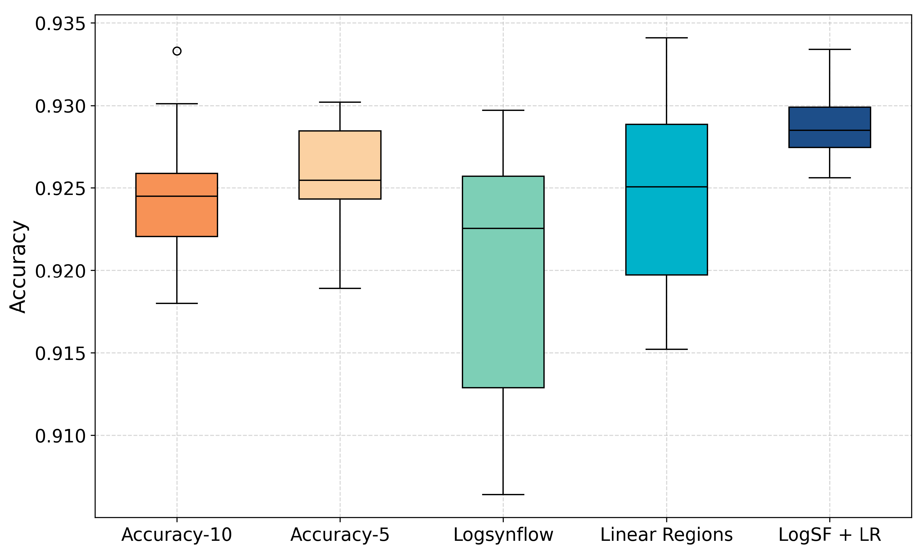Figure 5 presents a boxplot of the accuracy results. It is observed that the medians of the results are positioned closely. The Logsynflow configuration has the highest standard deviation, as shown in the respective box, which spans more than the other configurations.

The comparison presented in

Table 10. Average complexity of the resulting networks of the configurations of DeepGA with EEMs using the Fashion MNIST dataset. The standard deviation is shown in parentheses.

Configuration	No. Parameters	MFLOPS
Accuracy-10	243,438.0 (64,931.6)	140.3 (81.7)
Accuracy-5	247,103.6 (77,268.6)	156.0 (88.1)
Logsynflow	1,804,906.8 (636,449.4)	153.3 (179.5)
Linear Regions	1,442,433.2 (474,220.6)	1806.4 (755.9)
LogSF + LR	1,750,311.6 (471,406.5)	1306.6 (607.2)

corresponds to the average network complexity of the resulting models with the different configurations tested. The number of trainable parameters and the MFLOPS are included. It is observed that the training-free configurations resulted in networks with a considerably higher complexity. In the analysis of the MFLOPS, the Logsynflow configuration achieves a similar number of MFLOPS compared to the accuracy-based search. Conversely, the Linear Regions configuration and the combination of proxies have a considerably higher number of MFLOPS.

The effects of using the training-free proxies regarding the computational time are presented in

Table 11. Time comparison of the search process of DeepGA with EEMs using the Fashion MNIST dataset. The standard deviation is shown in parentheses.

Configuration	Evaluations	Search Time (h)	Diff (%)	Final Eval. (h)
Accuracy-10	226.8 (24.4)	17.071 (3.857)	-	0.389 (0.113)
Accuracy-5	231.9 (24.8)	9.220 (1.632)	45.99	0.384 (0.074)
Logsynflow	315.3 (27.2)	0.018 (0.002)	99.89	0.520 (0.178)
Linear Regions	295.9 (24.4)	0.028 (0.003)	99.84	2.009 (0.930)
LogSF + LR	311.8 (17.6)	0.032 (0.002)	99.81	1.589 (0.485)

. The training-free used more evaluations. Nonetheless, the search time reduction achieved by the zero-shot approach is above 99.81%. The training-free DeepGA completes the search in a matter of seconds. Regarding the final evaluation, it is observed that the Linear Regions proxy and the combined version with Logsynflow required more time to be completed. This observation aligns with being the architectures with considerably higher MFLOPS.

4.2.2. CIFAR-10

Table 12. DeepGA performance incorporating the training-free proxies to guide the search using the CIFAR-10 dataset. The best result is marked in bold.

Configuration	Best	Mean	Std Dev	Worst
Accuracy-10	0.8339	0.8145	0.0133	0.7840
Accuracy-5	0.8542	0.8290	0.0156	0.8094
Logsynflow	0.8083	0.7646	0.0257	0.7315
Linear Regions	0.8180	0.7853	0.0189	0.7643
LogSF + LR	0.8382	0.7800	0.0345	0.7416

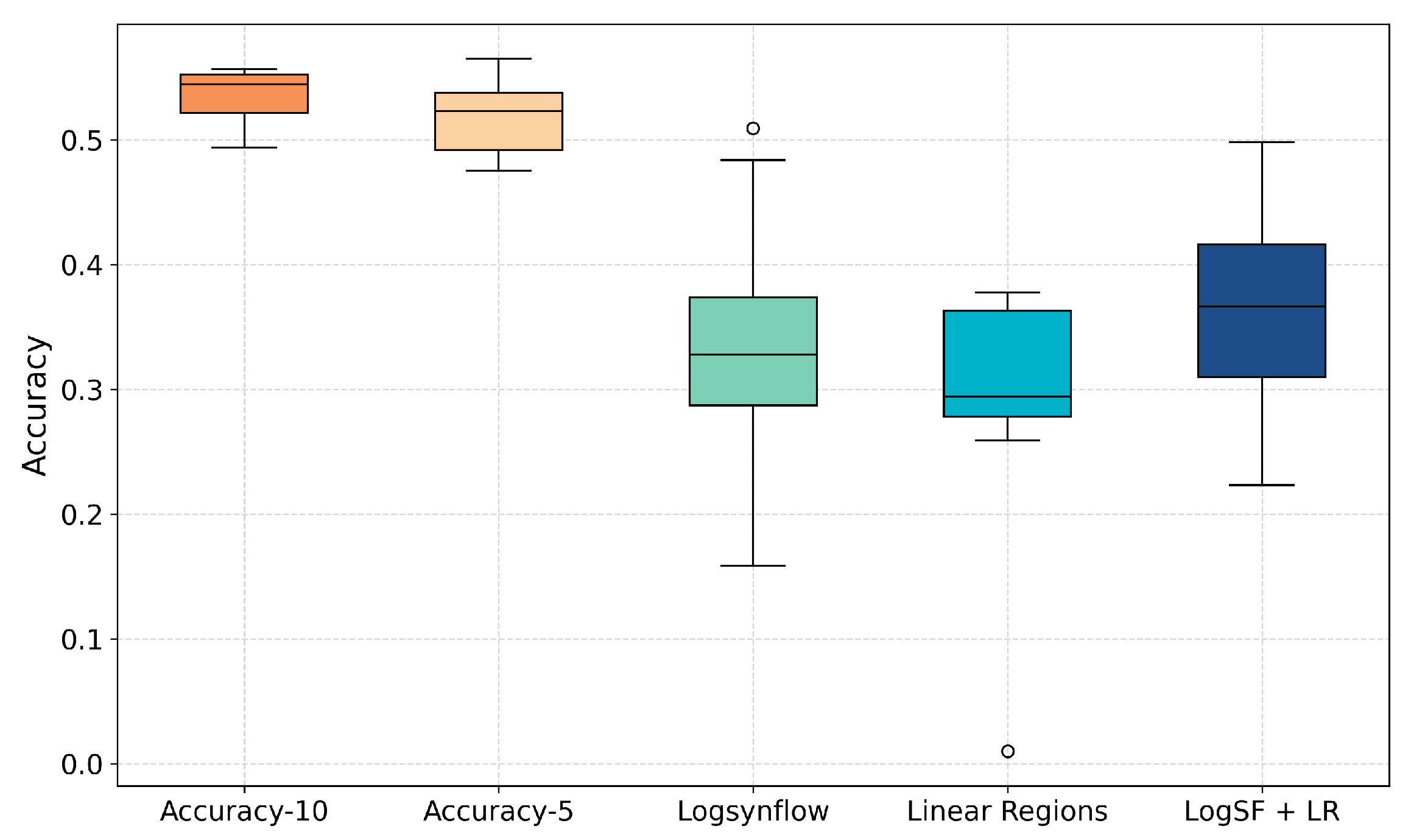
presents the accuracy performance of the different EEMs incorporated in DeepGA for the CIFAR-10 dataset. The highest values are obtained with the Accuracy-5 configuration. Figure 6 presents a box plot visualization of the results. It is seen that the accuracy-guided configurations are positioned above the training-free ones. In addition, Accuracy-10 and Accuracy-5 obtained the smallest standard deviation. An interesting point to observe is that the best result of the LogSf + LR configuration is higher than the best result from Accuracy-10. Statistical tests are conducted for a deeper analysis. The Friedman test detected significant differences among the means of the populations with a p-value of $2.18\times {10}^{-5}$.

The Nemenyi post-hoc test was used for a deeper analysis. The results are presented in

Table 13. Nemenyi post hoc analysis for the results with the CIFAR-10 dataset. The values where statistical differences are detected are marked in bold.

	Acc-10	Acc-5	Logsynflow	Linear Regions	LogSF + LR
Acc-10	1	0.8600	0.0062	0.1571	0.1141
Acc-5	0.8600	1	0.0001	0.0101	0.0062
Logsynflow	0.0062	0.0001	1	0.7899	0.8600
Linear Regions	0.1571	0.0101	0.7899	1	0.9999
LogSF + LR	0.1141	0.0062	0.8600	0.9999	1

. In this case, Accuracy-5 outperformed all the training-free configurations. On the other hand, the Accuracy-10 configuration only outmatched the Logsynflow configuration; no significant differences were detected when compared with the Linear Regions and the combined configurations. Unlike the reported pairwise comparison of the accuracy-guided search configurations, the Nemenyi post hoc procedure did not detect significant differences between using 5 or 10 training epochs during the search. Finally, there were no significant differences among the training-free configurations, i.e., no training-free configuration was better than the others.

Table 14. Average complexity of the resulting networks of the configurations of DeepGA with EEMs using the CIFAR-10 dataset. The standard deviation is shown in parentheses.

Configuration	No. Parameters	MFLOPS
Accuracy-10	660,554.8 (233,352.3)	232.0 (210.1)
Accuracy-5	842,744.4 (247,342.7)	350.6 (126.0)
Logsynflow	1,865,106.8 (504,233.2)	152.9 (260.7)
Linear Regions	1,748,256.4 (1,071,596.6)	2989.5 (1784.1)
LogSF + LR	1,884,343.6 (672,313.7)	1801.9 (1461.3)

presents the average complexity of the networks generated by DeepGA with the EEMs using the CIFAR-10 dataset. The trends are similar to those observed with the Fashion MNIST dataset. The training-free configurations present a considerably higher number of training parameters. Regarding the FLOPS, Linear Regions is again the configuration with the highest value, followed by the configuration with the combination of the training free proxies. Logsymflow required, on average, the least number of MFLOPS. The time comparison is presented in

Table 15. Time comparison of the search process of DeepGA with EEMs using the CIFAR-10 dataset. The standard deviation is shown in parentheses.

Configuration	Evaluations	Search Time (h)	Diff (%)	Final Eval. (h)
Accuracy-10	237.6 (18.8)	22.509 (4.682)	-	0.478 (0.187)
Accuracy-5	238.1 (28.5)	10.545 (3.237)	53.15	0.499 (0.197)
Logsynflow	291.2 (29.0)	0.017 (0.002)	99.92	0.468 (0.235)
Linear Regions	294.4 (28.5)	0.027 (0.003)	99.88	4.192 (2.152)
LogSF + LR	317.7 (15.9)	0.034 (0.003)	99.85	3.086 (3.575)

. The search time reduction achieved by the zero-shot search processes exceeds 99.8%. The final evaluation took considerably more time with the Linear Regions configuration and LogSF+LR, the configurations with the highest MFLOPS values.

4.2.3. CIFAR-100

The accuracy performance of the DeepGA configurations using EEMs is presented in

Table 16. DeepGA performance incorporating the training-free proxies to guide the search using the CIFAR-100 dataset. The best result is marked in bold.

Configuration	Best	Mean	Std Dev	Worst
Accuracy-10	0.5566	0.5341	0.0236	0.4938
Accuracy-5	0.5650	0.5173	0.0288	0.4749
Logsynflow	0.5093	0.3324	0.1111	0.1587
Linear Regions	0.3777	0.2889	0.1075	0.0100
LogSF + LR	0.4981	0.3644	0.0929	0.2232

, considering the CIFAR-100 dataset. It is seen that the best values are obtained with the accuracy-guided search. In this case, the Accuracy-10 is the configuration that has the highest mean value, but Accuracy-5 achieved the highest of the best values. An interesting behavior is observed in the worst cases of the training-free configurations with the CIFAR-100 dataset, where the search process resulted in architectures with particularly low performance. Figure 7 presents a box plot with the accuracy results. It is observed that the most compact boxes correspond to the accuracy-guided configurations, which are characterized by small standard deviation values. As shown in the figure, the worst result of the Linear Regions configuration, which exhibits poor performance, is an outlier.

Statistical tests were conducted. The Friedman test detected, with a p-value of $1.45\times {10}^{-5}$, that there are significant differences among the means of the results for the CIFAR-100 dataset. The Nemenyi post hoc procedure is then used. The details are presented in

Table 17. Nemenyi post hoc analysis for the results with the CIFAR-100 dataset. The values where statistical differences are detected are marked in bold.

	Acc-10	Acc-5	Logsynflow	Linear Regions	LogSF + LR
Acc-10	1	0.9153	0.0062	0.0002	0.0037
Acc-5	0.9153	1	0.0808	0.0062	0.0559
Logsynflow	0.0062	0.0808	1	0.9153	0.9999
Linear Regions	0.0002	0.0062	0.9153	1	0.9550
LogSF + LR	0.0037	0.0559	0.9999	0.9550	1

. It is seen that Accuracy-10 outperformed all of the training-free configurations. Nonetheless, no significant differences were detected when considering Accuracy-5 and the Logsynflow and LogSF + LR configurations. Additionally, no significant differences were observed among the training-free configurations.

The network complexity comparison for the CIFAR-100 datasets is presented in

Table 18. Average complexity of the resulting networks of the configurations of DeepGA with EEMs using the CIFAR-100 dataset. The standard deviation is shown in parentheses.

Configuration	No. Parameters	MFLOPS
Accuracy-10	1,159,852.0 (337,531.2)	457.9 (394.1)
Accuracy-5	1,420,398.4 (687,143.5)	258.1 (147.4)
Logsynflow	2,570,465.6 (428,558.4)	342.5 (225.2)
Linear Regions	1,863,878.4 (741,634.9)	3536.7 (1288.5)
LogSF + LR	1,766,450.4 (331,559.1)	1486.8 (852.3)

. Similarly to the other datasets, the trends in the number of parameters are that the training-free configurations resulted in higher network complexity. Nonetheless, the average number of parameters from Accuracy-5 is closer to the values of LogSf + LR than the same comparison with Fashion MNIST and CIFAR-10. The Linear Regions proxy exhibits consistent behavior in MFLOPS; it is again the configuration that requires a considerably higher number of MFLOPS.

Table 19. Time comparison of the search process of DeepGA with EEMs using the CIFAR-100 dataset. The standard deviation is shown in parentheses.

Configuration	Evaluations	Search Time (h)	Diff (%)	Final Eval. (h)
Accuracy-10	226.6 (27.4)	26.319 (13.664)	-	0.700 (0.492)
Accuracy-5	224.5 (31.7)	9.351 (2.910)	64.47	0.406 (0.115)
Logsynflow	327.2 (21.6)	0.020 (0.001)	99.92	0.811 (0.371)
Linear Regions	307.8 (17.4)	0.030 (0.003)	99.89	5.174 (2.067)
LogSF + LR	316.8 (23.3)	0.039 (0.005)	99.85	2.346 (1.303)

presents the time comparison for the CIFAR-100 dataset. The number of evaluations is higher in the training-free search process. However, the reduced cost of each evaluation in the zero-shot approaches is minimal compared to the accuracy-guided search. Therefore, the search time is immensely reduced by at least 97.42%. The final evaluations in the Linear Regions and LogSF + LR configurations are the most expensive.

4.3. Comparison of the Architectures

The first step in comparing the resulting architectures across different configurations of DeepGA with EEMs is to visualize the differences in the elements considered for the networks. Figure 8 presents the architectures from the best result of each configuration with the CIFAR-10 dataset (Table 12 presents their accuracy performance). The differences are evident. The accuracy-guided configurations considered resulted in architectures with no skip connections. The training-free search obtained deeper networks, which aligns with their larger number of parameters. The network with more convolutional layers (9) was the one obtained with the Linear Regions configuration. In addition, 15 skip connections were considered.

From Figure 8, the top-performing architecture is the one from Accuracy-5, which is the one presented in the figure with the smallest depth. The main difference between Accuracy-5 and Accuracy-10 in this case is the number of fully connected layers. The architecture with the second-best performance is the one from LogSF + LR, which features the most significant number of fully connected layers. The above observations demonstrate the difficulty in designing CNNs; there is a large number of possible designs and many paths that can be explored. Thus, the importance of NAS lies in automating the design process.

For a deeper understanding of the differences in the resulting architectures from the different DeepGA configurations, a comparison among their characteristics is presented in this subsection. For each architecture, the mean values of the following design and hyperparameter configurations are considered:

• Number of convolutional layers.
• Number of fully connected layers.
• Average number of filters per convolutional layer.
• Average filter size selected for the convolutional layers.
• Average number of neurons per fully connected layer.
• The frequency of using max pooling.
• The frequency of using average pooling.
• Average kernel size for pooling.
• Number of skip connections.

The results are presented in

Table 20. Mean values of network characteristics and hyperparameter configuration from the resulting architectures of applying DeepGA with EEMs using the Fashion MNIST dataset. The highest value is marked in bold as reference.

Configuration	Accuracy-10	Accuracy-5	Logsynflow	Linear Regions	LogSF + LR
No. Conv	4.3	4.6	7.1	6.7	6.7
No. FC	2.3	2.3	9.8	4.2	7.3
No. Filters/Conv	72.2	76.1	85.0	150.1	133.2
Mean Filter size	2.9	3.0	3.0	2.8	2.7
No. Neurons/FC	84.5	78.5	383.5	86.4	333.6
Freq Max pool	0.6	0.8	1.6	1.2	1.0
Freq Avg pool	0.7	0.6	1.2	0.8	0.8
Freq pool Off	3.0	3.2	4.3	4.7	4.9
Pooling kernel size	2.5	2.5	2.6	2.6	2.6
No. Skip Conns	1.8	2.0	5.2	3.4	5.1

for the Fashion MNIST dataset, in

Table 21. Mean values of network characteristics and hyperparameter configuration from the resulting architectures of applying DeepGA with EEMs using the CIFAR10 dataset. The highest value is marked in bold as reference.

Configuration	Accuracy-10	Accuracy-5	Logsynflow	Linear Regions	LogSF + LR
No. Conv	5.6	5.1	6.0	7.6	7.0
No. FC	3.0	2.8	9.1	3.5	9.1
No. Filters/Conv	119.3	127.7	71.2	149.9	125.5
Mean Filter size	3.2	3.0	3.3	2.7	2.9
No. Neurons/FC	154.1	97.4	429.6	112.9	302.1
Freq Max pool	1.4	1.5	1.3	0.9	0.8
Freq Avg pool	1.6	1.5	1.9	1.4	1.2
Freq pool Off	2.6	2.1	2.8	5.3	5.0
Pooling kernel size	2.5	2.6	2.5	2.5	2.3
No. Skip Conns	2.4	1.2	4.1	8.1	5.6

for CIFAR-10, and in

Table 22. Mean values of network characteristics and hyperparameter configuration from the resulting architectures of applying DeepGA with EEMs using the CIFAR-100 dataset. The highest value is marked in bold as reference.

Configuration	Accuracy-10	Accuracy-5	Logsynflow	Linear Regions	LogSF + LR
No. Conv	5.3	4.8	8.5	7.1	6.8
No. FC	1.5	1.4	11.7	4	7.2
No. Filters/Conv	119.2	129.0	79.8	168.8	138.7
Mean Filter size	2.8	3.0	3.1	2.5	2.6
No. Neurons/FC	317.9	337.1	403.5	57.9	336.2
Freq Max pool	1.4	2.4	1.5	0.6	1.3
Freq Avg pool	1.4	0.4	1.0	0.9	0.9
Freq pool Off	2.5	2.0	6.0	5.6	4.6
Pooling kernel size	2.5	2.6	2.6	2.3	2.5
No. Skip Conns	2.9	2.2	10.1	5.7	4.4

for the CIFAR-100 dataset.

The training-free configurations yielded deeper networks, featuring more convolutional and fully connected layers. Notably, it is observed that the accuracy-guided resulting architectures have a reduced number of fully connected layers, whereas the training-free configurations select more of them. With the accuracy-guided configurations, the primary difference observed between the configurations for the CIFAR-100 and CIFAR-10 datasets is the number of neurons in the fully connected layers. The previous explains the additional complexity of the CIFAR-100 architectures. Finally, the number of skip connections is considerably higher in the architectures from the training-free configurations.

Focusing on the number of filters per convolutional layer and the number of neurons in the fully connected ones, interesting patterns emerge. Linear Regions is the configuration that positions more filters on average in the convolutional layers. The behavior is consistent for the three datasets. In addition, Linear Regions positions a small number of neurons in the fully connected layers, as evident in the descriptions of the architectures for the CIFAR-100 dataset. On the other hand, Logsynflow consistently places more neurons in the fully connected layers and fewer filters in the convolutional layers. The combination of the proxies results in a middle point for both values.

5. Discussion

Early stopping, population memory, and training-free proxies are used in this paper as EEMs for NAS. Each of the mechanisms accelerated the search process of DeepGA in designing CNNs for image classification. First, as proposed in [29], 5 and 10 training epochs are used for the accuracy-based search process. The results showed that performing the search with only 5 epochs provides competitive results compared to the 10-epoch configuration. Consequently, time reductions of 45.99%, 64.47%, and 53.15% are achieved for Fashion MNIST, CIFAR-100, and CIFAR-10, respectively. Nonetheless, the resulting architecture is more complex with Accuracy-5.

Using the z-score normalization with a sigmoid function for scaling the training-free proxies resulted in a more consistent behavior than max normalization. The approach mentioned above enables the incorporation of training-free proxies into fitness functions that combine more than one proxy, as well as considering other design criteria, such as complexity limitations in DeepGA. The results showed that the training-free methods were partially competitive compared to the accuracy-guided search. The training-free methods were competitive with the Fashion MNIST data. In addition, no significant differences were detected in particular comparison cases, like Accuracy-5 and Logsynflow in CIFAR-100, or Linear Regions and Accuracy-10 in CIFAR-10. Nonetheless, in both datasets, an accuracy-based configuration outperformed all training-free configurations. It was observed that as the difficulty of the dataset increases, the proxies struggle to remain competitive.

No training-free configuration outperformed the others: using a combination of proxies does not yield better performance than using one of them independently. Nevertheless, it was observed that the resulting architectures from the combination of proxies presented trade-offs for particular network characteristics, such as the number of filters and number of neurons per convolutional and fully connected layers, respectively. The key point for using training-free proxies as EEMs is the expected high time reduction, which is confirmed in the results with a computational time reduction of above 99%. The comparison of the characteristics from the resulting architectures showed that the training-free configurations found deeper networks with considerably more fully connected layers and used more skip connections. Those network characteristics imply that training-free configurations tend to find more complex architectures than accuracy-based ones. Notably, the configurations that considered the Linear Regions proxy resulted in considerably more FLOPS than the other configurations, thereby increasing the time required for the final evaluation.

Lastly, the population memory mechanism enabled DeepGA to avoid more than 40% of the evaluations in the accuracy-based configurations and at least 20% of them in the training-free configurations. The percentage of avoided evaluations indicates the number of repeated architectures that the algorithm explores. It provides insights into the work of the selected variation operators of an EC algorithm and its parameter configuration.

6. Conclusions

This paper evaluates various EEMs in DeepGA, following an ENAS process that considers both accuracy-guided and training-free configurations. Early stopping resulted in competitive performance and considerable time reduction, highlighting the importance of selecting the number of training epochs in efficient NAS. The training-free option presented an extreme cost reduction but was only partially competitive in performance. Finally, population memory avoided repeated evaluations, resulting in further cost savings. Nonetheless, the findings are limited to three datasets, ten runs, and the consideration of only two different training-free proxies.

Future work is stated to extend the experimentation to other datasets and consider additional training-free search configurations and proxies. The focus is on improving the performance of the training-free NAS algorithm, particularly in cases where network complexity is limited. The use of a multi-objective configuration is also a proposed research direction. ENAS procedures can take advantage of the low cost of training-free proxies in the algorithm, utilizing a hybrid search process similar to surrogate models, where the expensive evaluation has limited use, while the low-cost evaluation is employed for exploration. Another possibility is considering the rich initialization of the algorithm’s population using training-free proxies to identify promising areas of the search space. Additionally, the lightweight proxies can be tested as a mechanism for parameter tuning in ENAS algorithms, where experimentation involves testing a series of parameter combinations.

References

1. Taye, M.M. Theoretical Understanding of Convolutional Neural Network: Concepts, Architectures, Applications, Future Directions. Computation 2023, 11, 52. [Google Scholar] [CrossRef]
2. Li, Z.; Liu, F.; Yang, W.; Peng, S.; Zhou, J. A Survey of Convolutional Neural Networks: Analysis, Applications, and Prospects. IEEE Trans. Neural Netw. Learn. Syst. 2022, 33, 6999–7019. [Google Scholar] [CrossRef] [PubMed]
3. Zhao, X.; Wang, L.; Zhang, Y.; Han, X.; Deveci, M.; Parmar, M. A review of convolutional neural networks in computer vision. Artif. Intell. Rev. 2024, 57, 99. [Google Scholar] [CrossRef]
4. Li, N.; Ma, L.; Xing, T.; Yu, G.; Wang, C.; Wen, Y.; Cheng, S.; Gao, S. Automatic design of machine learning via evolutionary computation: A survey. Appl. Soft Comput. 2023, 143, 110412. [Google Scholar] [CrossRef]
5. Telikani, A.; Tahmassebi, A.; Banzhaf, W.; Gandomi, A.H. Evolutionary Machine Learning: A Survey. ACM Comput. Surv. 2021, 54, 161. [Google Scholar] [CrossRef]
6. Li, N.; Ma, L.; Yu, G.; Xue, B.; Zhang, M.; Jin, Y. Survey on Evolutionary Deep Learning: Principles, Algorithms, Applications, and Open Issues. ACM Comput. Surv. 2023, 56, 41. [Google Scholar] [CrossRef]
7. Liu, Y.; Sun, Y.; Xue, B.; Zhang, M.; Yen, G.G.; Tan, K.C. A Survey on Evolutionary Neural Architecture Search. IEEE Trans. Neural Netw. Learn. Syst. 2023, 34, 550–570. [Google Scholar] [CrossRef] [PubMed]
8. Ren, P.; Xiao, Y.; Chang, X.; Huang, P.y.; Li, Z.; Chen, X.; Wang, X. A Comprehensive Survey of Neural Architecture Search: Challenges and Solutions. ACM Comput. Surv. 2021, 54, 76. [Google Scholar] [CrossRef]
9. Mishra, V.; Kane, L. A survey of designing convolutional neural network using evolutionary algorithms. Artif. Intell. Rev. 2023, 56, 5095–5132. [Google Scholar] [CrossRef]
10. Ünal, H.T.; Başçiftçi, F. Evolutionary design of neural network architectures: A review of three decades of research. Artif. Intell. Rev. 2022, 55, 1723–1802. [Google Scholar] [CrossRef]
11. Poyser, M.; Breckon, T.P. Neural architecture search: A contemporary literature review for computer vision applications. Pattern Recognit. 2024, 147, 110052. [Google Scholar] [CrossRef]
12. Song, X.; Xie, X.; Lv, Z.; Yen, G.G.; Ding, W.; Lv, J.; Sun, Y. Efficient Evaluation Methods for Neural Architecture Search: A Survey. IEEE Trans. Artif. Intell. 2024, 5, 5990–6011. [Google Scholar] [CrossRef]
13. Yang, S.; Tian, Y.; Xiang, X.; Peng, S.; Zhang, X. Accelerating Evolutionary Neural Architecture Search via Multifidelity Evaluation. IEEE Trans. Cogn. Dev. Syst. 2022, 14, 1778–1792. [Google Scholar] [CrossRef]
14. Sun, Y.; Xue, B.; Zhang, M.; Yen, G.G. Evolving Deep Convolutional Neural Networks for Image Classification. IEEE Trans. Evol. Comput. 2020, 24, 394–407. [Google Scholar] [CrossRef]
15. Liang, J.; Lou, Y.; Yu, M.; Bi, Y.; Yu, K. A survey of surrogate-assisted evolutionary algorithms for expensive optimization. J. Membr. Comput. 2024, 7, 108–127. [Google Scholar] [CrossRef]
16. Sun, Y.; Xue, B.; Zhang, M.; Yen, G.G.; Lv, J. Automatically Designing CNN Architectures Using the Genetic Algorithm for Image Classification. IEEE Trans. Cybern. 2020, 50, 3840–3854. [Google Scholar] [CrossRef] [PubMed]
17. Wu, M.T.; Tsai, C.W. Training-free neural architecture search: A review. ICT Express 2024, 10, 213–231. [Google Scholar] [CrossRef]
18. Li, G.; Hoang, D.; Bhardwaj, K.; Lin, M.; Wang, Z.; Marculescu, R. Zero-Shot Neural Architecture Search: Challenges, Solutions, and Opportunities. IEEE Trans. Pattern Anal. Mach. Intell. 2024, 46, 7618–7635. [Google Scholar] [CrossRef] [PubMed]
19. Cavagnero, N.; Robbiano, L.; Caputo, B.; Averta, G. FreeREA: Training-Free Evolution-based Architecture Search. In Proceedings of the 2023 IEEE/CVF Winter Conference on Applications of Computer Vision (WACV), Waikoloa, HI, USA, 2–7 January 2023; pp. 1493–1502. [Google Scholar] [CrossRef]
20. Mellor, J.; Turner, J.; Storkey, A.; Crowley, E.J. Neural Architecture Search without Training. In Proceedings of the 38th International Conference on Machine Learning, Virtual, 18–24 July 2021; Volume 139, pp. 7588–7598. [Google Scholar]
21. Wu, M.T.; Lin, H.I.; Tsai, C.W. A Training-Free Neural Architecture Search Algorithm Based on Search Economics. IEEE Trans. Evol. Comput. 2024, 28, 445–459. [Google Scholar] [CrossRef]
22. Wu, M.T.; Lin, H.I.; Tsai, C.W. A Training-free Genetic Neural Architecture Search. In Proceedings of the 2021 ACM International Conference on Intelligent Computing and Its Emerging Applications, Jinan, China, 28–29 December 2021; pp. 65–70. [Google Scholar] [CrossRef]
23. Hsieh, C.H.; Tsai, C.W. Rank-based Training-Free NAS Algorithm. In Proceedings of the 2023 International Conference on Intelligent Computing and Its Emerging Applications, Kaohsiung, Taiwan, 14–16 December 2023; pp. 30–35. [Google Scholar] [CrossRef]
24. Vo, A.; Pham, T.N.; Nguyen, V.B.; Luong, N.H. Training-Free Multi-Objective and Many-Objective Evolutionary Neural Architecture Search with Synaptic Flow. In Proceedings of the 11th International Symposium on Information and Communication Technology, Hanoi, Vietnam, 1–3 December 2022; pp. 1–8. [Google Scholar] [CrossRef]
25. Luong, N.H.; Phan, Q.M.; Vo, A.; Pham, T.N.; Bui, D.T. Lightweight multi-objective evolutionary neural architecture search with low-cost proxy metrics. Inf. Sci. 2024, 655, 119856. [Google Scholar] [CrossRef]
26. Ying, C.; Klein, A.; Christiansen, E.; Real, E.; Murphy, K.; Hutter, F. NAS-Bench-101: Towards Reproducible Neural Architecture Search. In Proceedings of the 36th International Conference on Machine Learning, Long Beach, CA, USA, 9–15 June 2019; Volume 97, pp. 7105–7114. [Google Scholar]
27. Thanh, T.H.; Doan, L.; Luong, N.H.; Huynh Thi Thanh, B. THNAS-GA: A Genetic Algorithm for Training-free Hardware-aware Neural Architecture Search. In Proceedings of the Genetic and Evolutionary Computation Conference, Melbourne, Australia, 14–18 July 2024; pp. 1128–1136. [Google Scholar] [CrossRef]
28. Lin, J.C.; Tsai, C.W. A Lightweight Training-Free Method for Neural Architecture Search. In Proceedings of the 2024 IEEE Congress on Evolutionary Computation (CEC), Yokohama, Japan, 30 June–5 July 2024; pp. 1–8. [Google Scholar] [CrossRef]
29. Barradas-Palmeros, J.A.; López-Herrera, C.A.; Acosta-Mesa, H.G.; Mezura-Montes, E. Efficient Neural Architecture Search: Computational Cost Reduction Mechanisms in DeepGA. In Advances in Computational Intelligence. Proceedings of the MICAI 2024 International Workshops, Tonantzintla, Mexico, 21–25 October 2024; Martínez-Villaseñor, L., Ochoa-Ruiz, G., Montes Rivera, M., Barrón-Estrada, M.L., Acosta-Mesa, H.G., Eds.; Springer: Cham, Switzerland, 2025; pp. 125–134. [Google Scholar] [CrossRef]
30. Vargas-Hákim, G.A.; Mezura-Montes, E.; Acosta-Mesa, H.G. Hybrid encodings for neuroevolution of convolutional neural networks: A case study. In Proceedings of the Genetic and Evolutionary Computation Conference Companion, Lille, France, 10–14 July 2021; pp. 1762–1770. [Google Scholar] [CrossRef]
31. Llaguno-Roque, J.L.; Barrientos-Martínez, R.E.; Acosta-Mesa, H.G.; Romo-González, T.; Mezura-Montes, E. Neuroevolution of Convolutional Neural Networks for Breast Cancer Diagnosis Using Western Blot Strips. Math. Comput. Appl. 2023, 28, 72. [Google Scholar] [CrossRef]
32. Vázquez-Santiago, D.I.; Acosta-Mesa, H.G.; Mezura-Montes, E. Vehicle Make and Model Recognition as an Open-Set Recognition Problem and New Class Discovery. Math. Comput. Appl. 2023, 28, 80. [Google Scholar] [CrossRef]
33. Morales-Reyes, J.L.; Aquino-Bolaños, E.N.; Acosta-Mesa, H.G.; Márquez-Grajales, A. Estimation of Anthocyanins in Heterogeneous and Homogeneous Bean Landraces Using Probabilistic Colorimetric Representation with a Neuroevolutionary Approach. Math. Comput. Appl. 2024, 29, 68. [Google Scholar] [CrossRef]
34. Velazco-Muñoz, J.D.; Acosta-Mesa, H.G.; Mezura-Montes, E. Reducing Parameters by Neuroevolution in CNN for Steering Angle Estimation. In Pattern Recognition. Proceedings of the MCPR 2024, Xalapa, Mexico, 19–22 June 2024; Mezura-Montes, E., Acosta-Mesa, H.G., Carrasco-Ochoa, J.A., Martínez-Trinidad, J.F., Olvera-López, J.A., Eds.; Springer: Cham, Switzerland, 2024; pp. 377–386. [Google Scholar]
35. Xiao, H.; Rasul, K.; Vollgraf, R. Fashion-MNIST: A Novel Image Dataset for Benchmarking Machine Learning Algorithms. arXiv 2017, arXiv:1708.07747v2. [Google Scholar] [CrossRef]
36. Krizhevsky, A. Learning Multiple Layers of Features from Tiny Images; Technical Report; Computer Science Department, University of Toronto: Toronto, ON, Canada, 2009. [Google Scholar]
37. Bolón-Canedo, V.; Morán-Fernández, L.; Cancela, B.; Alonso-Betanzos, A. A review of green artificial intelligence: Towards a more sustainable future. Neurocomputing 2024, 599, 128096. [Google Scholar] [CrossRef]
38. Vargas-Hákim, G.A.; Mezura-Montes, E.; Acosta-Mesa, H.G. A Review on Convolutional Neural Network Encodings for Neuroevolution. IEEE Trans. Evol. Comput. 2022, 26, 12–27. [Google Scholar] [CrossRef]
39. Deb, K.; Pratap, A.; Agarwal, S.; Meyarivan, T. A fast and elitist multiobjective genetic algorithm: NSGA-II. IEEE Trans. Evol. Comput. 2002, 6, 182–197. [Google Scholar] [CrossRef]
40. Tanaka, H.; Kunin, D.; Yamins, D.L.; Ganguli, S. Pruning neural networks without any data by iteratively conserving synaptic flow. In Proceedings of the Advances in Neural Information Processing Systems, Virtual, 6–12 December 2020; Volume 33, pp. 6377–6389. [Google Scholar]
41. Paszke, A.; Gross, S.; Massa, F.; Lerer, A.; Bradbury, J.; Chanan, G.; Killeen, T.; Lin, Z.; Gimelshein, N.; Antiga, L.; et al. PyTorch: An imperative style, high-performance deep learning library. In Proceedings of the 33rd International Conference on Neural Information Processing Systems, Vancouver, BC, Canada, 8–14 December 2019. [Google Scholar]
Figure 1. An example of the neural encoding of DeepGA. Two levels are used. The first level consists of convolutional (square) and fully connected (circle) blocks, along with the details of each layer. In the second level, skip connections are considered. The second level encoding in the figure represents no skip connections to the third convolutional layer, a skip connection from the output of the first layer to the input of the fourth layer, and skip connections from the second and third layers to the fifth layer.
Mca 30 00074 g001
Figure 2. An example of the crossover procedure in DeepGA. The operator works on two levels, taking two parents as input and returning two individuals as offspring. First, a fraction of the blocks is exchanged, and then, a portion of the bits in the bit string is swapped.
Mca 30 00074 g002
Figure 3. Mutation of restarting a block applied when r 1 0.5 .
Mca 30 00074 g003
Figure 4. Mutation of adding one block applied when r 1 < 0.5 .
Mca 30 00074 g004
Figure 5. Boxplot of the accuracy performance of the accuracy-guided and training-free search in DeepGA using the Fashion MNIST dataset.
Mca 30 00074 g005
Figure 6. Boxplot of the accuracy performance of the accuracy-guided and training-free search in DeepGA using the CIFAR-10 dataset.
Mca 30 00074 g006
Figure 7. Boxplot of the accuracy performance of the accuracy-guided and training-free search in DeepGA using the CIFAR-100 dataset.
Mca 30 00074 g007
Figure 8. Representation of the best performing architectures obtained with the different DeepGA configurations. The square blocks represent convolutional layers; their number of filters and pooling type are displayed under the block. Circles represent fully-connected blocks, and the number of neurons is displayed below the block.
Mca 30 00074 g008