Figure 1.
Common bean landraces with homogeneous and heterogeneous seeds. Bean landraces with (A) yellow color seeds (homogeneous), (B) black and red color seeds (heterogeneous), (C) black, yellow and pink color seeds (heterogeneous), (D) variegated seeds (heterogeneous), and (E) yellow and variegated seeds (heterogeneous).
Figure 2.
Color categories considered for seeds.
Figure 2.
Color categories considered for seeds.
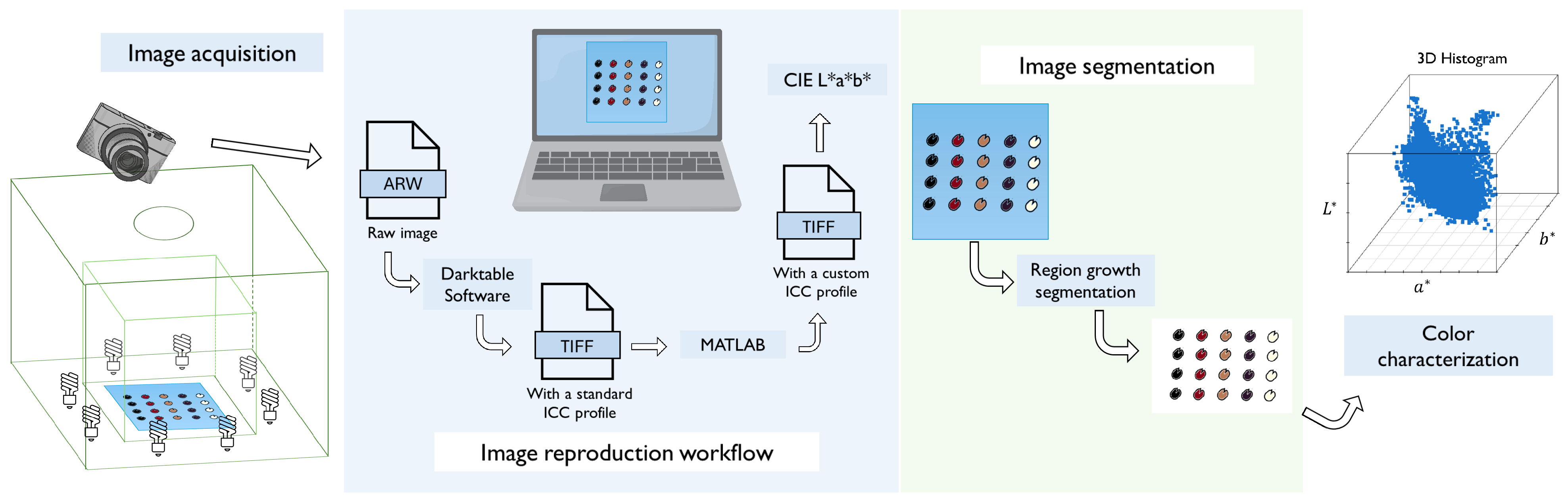
Figure 3.
Process performed to obtain the color information of the bean landraces seeds as 3D histograms in the CIE L*a*b* color space.
Figure 3.
Process performed to obtain the color information of the bean landraces seeds as 3D histograms in the CIE L*a*b* color space.
Figure 4.
Prototype for the image acquisition process.
Figure 4.
Prototype for the image acquisition process.
Figure 5.
Visual contrast between the bean landrace and the background of the image in blue color.
Figure 5.
Visual contrast between the bean landrace and the background of the image in blue color.
Figure 6.
CIE L*a*b* color space.
Figure 6.
CIE L*a*b* color space.
Figure 7.
Original and binary image obtained with the region growth segmentation algorithm. The black regions obtained correspond to the region of interest, i.e., the bean landrace seeds.
Figure 7.
Original and binary image obtained with the region growth segmentation algorithm. The black regions obtained correspond to the region of interest, i.e., the bean landrace seeds.
Figure 8.
3D histogram divisions considering the CIE L*a*b* color space.
Figure 8.
3D histogram divisions considering the CIE L*a*b* color space.
Figure 9.
3D histogram of a bean landrace in the CIE L*a*b* color space.
Figure 9.
3D histogram of a bean landrace in the CIE L*a*b* color space.
Figure 10.
Example of (a) a dataset dispersion in , and (b) its corresponding fitted Gaussian mixture distribution.
Figure 10.
Example of (a) a dataset dispersion in , and (b) its corresponding fitted Gaussian mixture distribution.
Figure 11.
Graphical representation of a joint distribution function whose projections onto the axes are the distributions and .
Figure 11.
Graphical representation of a joint distribution function whose projections onto the axes are the distributions and .
Figure 12.
Process of data cleansing using thresholding on a 3D histogram of a bean landrace. (A) presents the positions considered in the original 3D histogram and (B) the positions that remain after the thresholding process.
Figure 12.
Process of data cleansing using thresholding on a 3D histogram of a bean landrace. (A) presents the positions considered in the original 3D histogram and (B) the positions that remain after the thresholding process.
Figure 13.
Bean landraces with seeds of heterogeneous colors, considering one, two or three colors in each landrace.
Figure 13.
Bean landraces with seeds of heterogeneous colors, considering one, two or three colors in each landrace.
Figure 14.
Example of the steps performed for the general design of the experiments. The training dataset (A) is structured by the single-point means of 3D histograms of individual seeds that have been labeled with one of seven colors considered. The test dataset (B) comprises the means with a mixture proportion greater than zero delivered by the GI algorithm for the bean landraces analyzed. The labels predicted by the K- method for the test dataset (C) are obtained, and the label assignment for each bean landrace (D) is considered as the set of colors identified by the K- method in their respective means. To evaluate the performance of the proposed method, the precision of each bean landrace, , and the general precision, , (E), are considered.
Figure 15.
Process performed in one bean landrace seed of homogeneous color to obtain its representative mean in the CIE L*a*b* color space.
Figure 15.
Process performed in one bean landrace seed of homogeneous color to obtain its representative mean in the CIE L*a*b* color space.
Figure 16.
Example of the representative means for a training dataset in the CIE L*a*b* color space.
Figure 16.
Example of the representative means for a training dataset in the CIE L*a*b* color space.
Figure 17.
Process performed in one bean landrace of heterogeneous color to obtain its representative means in the CIE L*a*b* color space.
Figure 17.
Process performed in one bean landrace of heterogeneous color to obtain its representative means in the CIE L*a*b* color space.
Figure 18.
Boxplots of the results obtained considering bean landraces with one- and two-color seeds and the different K values for the K- method with the proposed methodology, fitting 7 Gaussians with the GI algorithm. The median for each K value is displayed in the corresponding boxplot.
Figure 18.
Boxplots of the results obtained considering bean landraces with one- and two-color seeds and the different K values for the K- method with the proposed methodology, fitting 7 Gaussians with the GI algorithm. The median for each K value is displayed in the corresponding boxplot.
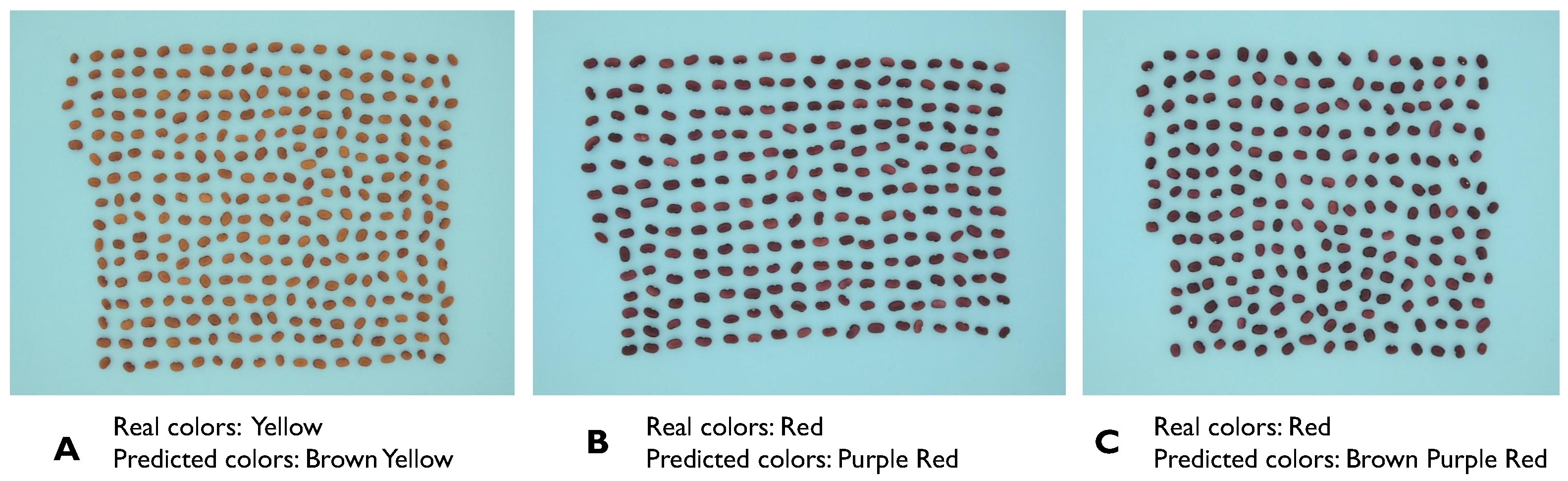
Figure 19.
Examples of bean landraces with single-color seeds (according to the expert), where the proposed methodology identifies the color, and one (A,B) or two colors more (C).
Figure 19.
Examples of bean landraces with single-color seeds (according to the expert), where the proposed methodology identifies the color, and one (A,B) or two colors more (C).
Figure 20.
Examples of bean landraces characterized by the presence of two colors on their seeds (according to the expert), where the proposed methodology identifies these colors and one more color.
Figure 20.
Examples of bean landraces characterized by the presence of two colors on their seeds (according to the expert), where the proposed methodology identifies these colors and one more color.
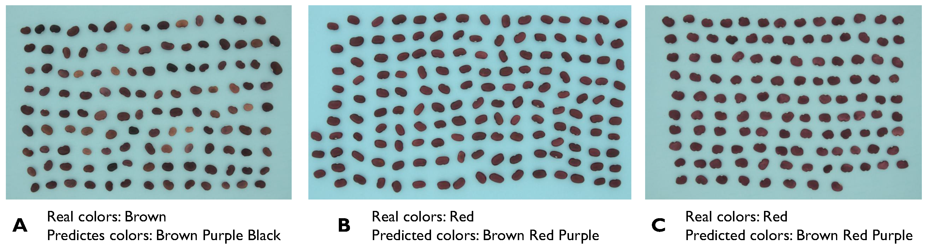
Figure 21.
Examples of bean landraces characterized by the presence of two colors on their seeds (according to the expert), where the proposed methodology identifies these colors and two more colors.
Figure 21.
Examples of bean landraces characterized by the presence of two colors on their seeds (according to the expert), where the proposed methodology identifies these colors and two more colors.
Figure 22.
Examples of bean landraces characterized by the presence of two colors on their seeds (according to the expert), where the proposed methodology only identifies one of these colors.
Figure 22.
Examples of bean landraces characterized by the presence of two colors on their seeds (according to the expert), where the proposed methodology only identifies one of these colors.
Figure 23.
Examples of bean landraces characterized by the presence of two colors on their seeds (according to the expert), where the proposed methodology only identifies one of these colors and assigns two colors (A,B) or one color (C) more.
Figure 23.
Examples of bean landraces characterized by the presence of two colors on their seeds (according to the expert), where the proposed methodology only identifies one of these colors and assigns two colors (A,B) or one color (C) more.
Figure 24.
Boxplots of the results obtained considering bean landraces with one-, two-, and three-color seeds and the different K values for the K- method with the proposed methodology, and fitting 7 Gaussians with the GI algorithm. The median for each K value is displayed in the corresponding boxplot.
Figure 25.
Examples of bean landraces where the real color observed by the expert is included in the corresponding set of predicted colors with the proposed methodology, with two colors.
Figure 25.
Examples of bean landraces where the real color observed by the expert is included in the corresponding set of predicted colors with the proposed methodology, with two colors.
Figure 26.
Examples of bean landraces where the real color observed by the expert is included in the corresponding set of predicted colors with the proposed methodology, with three colors.
Figure 26.
Examples of bean landraces where the real color observed by the expert is included in the corresponding set of predicted colors with the proposed methodology, with three colors.
Figure 27.
Examples of bean landraces where the real color observed by the expert is included in the corresponding set of predicted colors with the proposed methodology, with four colors.
Figure 27.
Examples of bean landraces where the real color observed by the expert is included in the corresponding set of predicted colors with the proposed methodology, with four colors.
Figure 28.
Examples of bean landraces where the two real colors observed by the expert are included in the corresponding set of predicted colors with the proposed methodology, with three colors.
Figure 28.
Examples of bean landraces where the two real colors observed by the expert are included in the corresponding set of predicted colors with the proposed methodology, with three colors.
Figure 29.
Examples of bean landraces where the two real colors observed by the expert are included in the corresponding set of predicted colors with the proposed methodology, with four colors.
Figure 29.
Examples of bean landraces where the two real colors observed by the expert are included in the corresponding set of predicted colors with the proposed methodology, with four colors.
Figure 30.
Examples of bean landraces where the three real colors observed by the expert are included in the corresponding set of predicted colors with the proposed methodology, with four colors.
Figure 30.
Examples of bean landraces where the three real colors observed by the expert are included in the corresponding set of predicted colors with the proposed methodology, with four colors.
Figure 31.
Bean landrace where the three real colors observed by the expert are included in the corresponding set of predicted colors with the proposed methodology, with five colors.
Figure 31.
Bean landrace where the three real colors observed by the expert are included in the corresponding set of predicted colors with the proposed methodology, with five colors.
Figure 32.
Examples of bean landraces where the predicted color with the proposed methodology is included in the corresponding set of real colors observed by the expert, with three colors.
Figure 32.
Examples of bean landraces where the predicted color with the proposed methodology is included in the corresponding set of real colors observed by the expert, with three colors.
Figure 33.
Examples of bean landraces where the two predicted colors with the proposed methodology are included in the corresponding set of real colors observed by the expert, with three colors.
Figure 33.
Examples of bean landraces where the two predicted colors with the proposed methodology are included in the corresponding set of real colors observed by the expert, with three colors.
Figure 34.
Examples of bean landraces where the set of predicted colors with the proposed methodology and the set of real colors observed by the expert have one or two colors in common.
Figure 34.
Examples of bean landraces where the set of predicted colors with the proposed methodology and the set of real colors observed by the expert have one or two colors in common.
Figure 35.
Examples of training datasets considered in the experiments of the proposed methodology.
Figure 35.
Examples of training datasets considered in the experiments of the proposed methodology.
Table 1.
Number of bean landraces that have one, two, or three colors on their seeds.
Table 1.
Number of bean landraces that have one, two, or three colors on their seeds.
| Number of Colors | Number of Landraces |
|---|
| One | 130 |
| Two | 42 |
| Three | 34 |
| Total | 206 |
Table 2.
Number of bean landrace seeds used in the experimental setup and training dataset, categorized by color.
Table 2.
Number of bean landrace seeds used in the experimental setup and training dataset, categorized by color.
| Color | Number of Seeds | Number of Seeds for Training (10%) |
|---|
| Black | 108 | 11 * |
| Brown | 135 | 14 * |
| Pink | 48 | 5 * |
| Purple | 110 | 11 |
| Red | 166 | 17 * |
| White | 66 | 7 * |
| Yellow | 129 | 13 * |
| Total | 762 | 78 |
Table 3.
Computer specifications.
Table 3.
Computer specifications.
| Operating System | Windows 11 Pro 23H2 |
|---|
| RAM | 64 GB |
| Processor | AMD Ryzen 5 5600G |
| Processor speed | 3.90 GHz |
Table 4.
Results of the experiments considering bean landraces with seeds of one and two colors, searching for 7 Gaussian components with the GI algorithm.
Table 4.
Results of the experiments considering bean landraces with seeds of one and two colors, searching for 7 Gaussian components with the GI algorithm.
| K | Min | Max | Mean ± St.D. | Train/Test Mean Time (min) | p-Value (Shapiro-Wilk) |
|---|
| 1 | 0.7209 | 0.9477 | 0.8974 ± 0.0651 | 4.05/8.67 | 2.51 × 10⁻⁵ * |
| 2 | 0.7384 | 0.9419 | 0.9041 ± 0.0437 | 4.34/8.40 | 1.50 × 10⁻⁵ * |
| 3 | 0.7529 | 0.9477 | 0.8953 ± 0.0645 | 4.17/8.45 | 3.16 × 10⁻⁵ * |
| 4 | 0.7616 | 0.9506 | 0.9161 ± 0.0414 | 4.04/8.45 | 1.88 × 10⁻⁵ * |
| 5 | 0.7878 | 0.9477 | 0.9164 ± 0.0400 | 4.18/8.47 | 2.37 × 10⁻⁶ * |
| 6 | 0.8488 | 0.9477 | 0.9256 ± 0.0236 | 4.06/8.42 | 3.46 × 10⁻⁵ * |
| 7 | 0.8256 | 0.9564 | 0.9230 ± 0.0279 | 4.07/8.46 | 5.92 × 10⁻⁴ * |
| 8 | 0.7471 | 0.9622 | 0.9231 ± 0.0435 | 4.09/8.48 | 5.09 × 10⁻⁷ * |
| 9 | 0.7500 | 0.9622 | 0.9259 ± 0.0437 | 4.12/8.50 | 6.95 × 10⁻⁷ * |
| 10 | 0.8692 | 0.9506 | 0.9279 ± 0.0192 | 4.16/8.52 | 8.05 × 10⁻³ * |
Table 5.
Analysis of labels obtained with the proposed methodology considering bean landraces with one- and two-color seeds.
Table 5.
Analysis of labels obtained with the proposed methodology considering bean landraces with one- and two-color seeds.
| Description | Number of Bean Landraces |
|---|
| Same colors | 99 |
| Predicted colors contain real colors | 60 |
| Real colors contain predicted colors | 3 |
| Some colors are the same | 10 |
| Different colors | 0 |
| Total | 172 |
Table 6.
Analysis of bean landraces where the real colors are contained in the predicted colors.
Table 6.
Analysis of bean landraces where the real colors are contained in the predicted colors.
| Real Colors | Predicted Colors | Number of Bean Landraces |
|---|
| 1 | 2 | 33 |
| 1 | 3 | 7 |
| 2 | 3 | 16 |
| 2 | 4 | 4 |
Table 7.
Results of the experiments considering bean landraces with seeds of one, two and three colors, searching for 7 Gaussian components with the GI algorithm.
Table 7.
Results of the experiments considering bean landraces with seeds of one, two and three colors, searching for 7 Gaussian components with the GI algorithm.
| K | Min | Max | Mean ± St.D. | Train/Test Mean Time (min) | p-Value (Shapiro-Wilk) |
|---|
| 1 | 0.6610 | 0.8989 | 0.8408 ± 0.0656 | 4.17/10.37 | 9.56 × 10⁻⁵ * |
| 2 | 0.6731 | 0.8859 | 0.8459 ± 0.0564 | 4.19/10.36 | 1.73 × 10⁻⁵ * |
| 3 | 0.6683 | 0.8859 | 0.8503 ± 0.0568 | 4.32/10.38 | 3.37 × 10⁻⁶ * |
| 4 | 0.6820 | 0.8908 | 0.8590 ± 0.0524 | 4.29/10.42 | 1.12 × 10⁻⁶ * |
| 5 | 0.7112 | 0.9094 | 0.8704 ± 0.0403 | 4.19/10.47 | 1.64 × 10⁻⁶ * |
| 6 | 0.7751 | 0.8997 | 0.8725 ± 0.0268 | 4.20/10.50 | 1.04 × 10⁻⁴ * |
| 7 | 0.7961 | 0.9037 | 0.8765 ± 0.0235 | 4.34/10.50 | 9.22 × 10⁻⁴ * |
| 8 | 0.8139 | 0.9013 | 0.8741 ± 0.0207 | 4.20/10.51 | 8.09 × 10⁻³ * |
| 9 | 0.8390 | 0.9013 | 0.8765 ± 0.0166 | 4.27/10.60 | 3.30 × 10⁻¹ * |
| 10 | 0.8341 | 0.8989 | 0.8739 ± 0.0173 | 4.29/10.64 | 2.94 × 10⁻¹ * |
Table 8.
Analysis of labels obtained with the proposed methodology considering bean landraces with one-, two-, and three-color seeds.
Table 8.
Analysis of labels obtained with the proposed methodology considering bean landraces with one-, two-, and three-color seeds.
| Description | Number of Bean Landraces |
|---|
| Same colors | 118 |
| Predicted colors contain real colors | 47 |
| Real colors contain predicted colors | 9 |
| Some colors are the same | 32 |
| Different colors | 0 |
| Total | 206 |
Table 9.
Analysis of bean landraces where the real colors are contained in the predicted colors.
Table 9.
Analysis of bean landraces where the real colors are contained in the predicted colors.
| Real Colors | Predicted Colors | Number of Bean Landraces |
|---|
| 1 | 2 | 18 |
| 1 | 3 | 5 |
| 1 | 4 | 3 |
| 2 | 3 | 11 |
| 2 | 4 | 5 |
| 3 | 4 | 4 |
| 3 | 5 | 1 |
Table 10.
Analysis of bean landraces where the predicted colors are contained in the real colors.
Table 10.
Analysis of bean landraces where the predicted colors are contained in the real colors.
| Real Colors | Predicted Colors | Number of Bean Landraces |
|---|
| 3 | 1 | 2 |
| 3 | 2 | 7 |

 ,
, 


