Multiple-Feature Construction for Image Segmentation Based on Genetic Programming

Abstract

Within the medical field, computer vision has an important role in different tasks, such as health anomaly detection, diagnosis, treatment, and monitoring medical conditions. Image segmentation is one of the most used techniques for medical support to identify regions of interest in different organs. However, performing accurate segmentation is difficult due to image variations. In this way, this work proposes an automated multiple-feature construction approach for image segmentation, working with magnetic resonance images, computed tomography, and RGB digital images. Genetic programming is used to automatically create and construct pipelines to extract meaningful features for segmentation tasks. Additionally, a co-evolution strategy is proposed within the evolution process to increase diversity without affecting segmentation performance. The segmentation is addressed as a pixel classification task; in this way, a wrapper approach is used, and the classification model’s segmentation performance determines the fitness. To validate the effectiveness of the proposed method, four datasets were used to measure the capability of the proposal to deal with different types of medical images. The results demonstrate that the proposal achieves values of the DICE similarity coefficient of more than 0.6 in MRI and C.T. images. Additionally, the proposal is compared with SOTA GP-based methods and the convolutional neural networks used within the medical field. The method proposed outperforms these methods, achieving improvements greater than $20\%$ in DICE, specificity, and sensitivity. Additionally, the qualitative results demonstrate that the proposal accurately identifies the region of interest.

1. Introduction

Computer vision has been an important and relevant tool within the medical field. The capabilities of computer vision systems that involve images play an important role in clinical care and treatment. Also, these systems can support medical staff and decision-making, particularly for personnel with limited experience. Furthermore, medical images can effectively help doctors evaluate the size of different disease tumors and analyze the images obtained before and after treatment. Numerous approaches for different tasks have been developed over the last several years, such as image classification [1,2,3,4,5,6], image segmentation [7,8,9,10,11,12], and image estimation [13]. These tasks involve medical imaging, and typically, the images used are obtained via Magnetic Resonance Imaging (MRI), X-ray, and Computerized Tomography (C.T.) [14]. Working with medical imaging, grayscale images are commonly used because most medical image acquisition systems naturally produce grayscale output based on intensity values corresponding to tissue density or signal response [15]. The grayscale comprises an image where each pixel can take a value between 0 and 255. The lowest value (0) represents black, and the highest (255) represents white.

The segmentation process separates an image into representative regions according to certain criteria shared in a specific area. It differentiates digital image pixels belonging to an object from those corresponding to the background [7]. Image segmentation has several grades of complexity according to the different coarse and fine granularities of segmentation [3]. The lowest complexity is the semantic segmentation, where each pixel has a label that determines whether it belongs to the object [16], also known as binary segmentation. For example, the task is to identify an object from the rest of the image. The medium complexity is the instance segmentation, which allocates a pixel label for objects and separates them from each other; in other words, it separates the per-object mask and localizes varying numbers of instances presented in the image [17], for example, when identifying cars in traffic, each vehicle has its own label. The highest complexity is panoptic segmentation, which generalizes and combines instance segmentation and semantic segmentation. The task is to identify individual objects and their backgrounds, for example, to identify trees in a landscape and also the sky or the ground [18].

To perform these tasks adequately, the object/interest region needs to be separated from the background, which is not an easy task. Firstly, one of the most common issues is the low quality or noise within the images caused by the acquisition of the source device. In this way, noise can influence determining which region belongs to the background and the Region Of Interest (ROI). Secondly, determining which techniques or functions of image processing are the most adequate to perform the segmentation requires expertise.

Several approaches have been proposed within the state of the art. The well-known convolutional neural networks are the most popular deep learning models, such as U-net [9] and U-net++ [19]. These architectures are relevant within the medical field, which is the interest of this research. Despite the good performance of these models, designing and implementing them requires knowledge about artificial neural networks. Additionally, they are known as “black boxes”, and the big models lack information about how they perform tasks, making it difficult for humans to analyze and interpret the procedure. However, several efforts have been reported in the area of evolutionary computation (EC), specifically within the field of Genetic Programming (GP) for image classification and segmentation, where the approaches work as “white boxes” [20].

In this way, this work proposes an automated approach for multiple-feature construction for medical image segmentation. Based on Darwin’s metaphor, evolutionary computation is employed to perform a guided search for selecting image processing functions such as filters, morphological operators, and pixel operations, which modify the raw data until meaningful features are extracted. Selecting by hand the set of functions for feature extraction in the images requires effort and is time-consuming. In contrast, the automated approach for multiple-feature construction significantly reduces processing time, improves efficiency and precision, and allows for adaptation using different images. For this reason, the automated approach for multiple-feature construction saves time in the trial and error phases.

The proposed approach, Genetic Programming Multiple-Image Feature Construction (GP-MIFC), extracts five different features from the raw images, and then the segmentation is performed as a pixel classification task. In this way, a classification model is employed in the pipeline. The contributions of this research can be summarized as follows:

• Multiple features are constructed independently from the raw grayscale images.
• A co-evolution strategy is adapted to evolve five different populations, and each one constructs a feature used for the segmentation step.
• The binarization for segmentation is performed as a pixel classification task using an Iterative Dichotomiser 3 (ID3) classifier [21].
• Images are segmented from different acquisition systems such as Computed Tomography (C.T.), Magnetic Resonance Imaging (M.R.I.), and digital images.

2. Background and Related Work

2.1. Basics of Genetic Programming

GP is a paradigm of EC known for evolving computer programs. It has gained relevance in recent years due to its capability to deal with problems in different research areas mainly due to its flexibility to adapt problems to tree representations, including complex functions or computer programs. Additionally, it enhances the transparency of the solutions, making them more interpretable for humans. Each solution is easy to replicate via analysis. Furthermore, unlike other optimization techniques based on the gradient, GP can be optimized in non-differentiable or discontinuous functions. GP can be considered as an automated learning method—the evolutionary process supports the automatic search.

The paradigm of GP is based on Darwin’s evolutionary theory, where a population of programs (individuals) lives within a specific environment. Within this environment, the individuals contend among themselves, and those that perform better according to the environmental conditions are selected for reproduction. This selection process ensures that the individuals with the highest fitness and who are most capable of solving problems have a high probability of producing offspring.

The offspring inherit features from their parents with some variations. Through generations, the offspring will be able to adapt to the environment, ensuring that future generations evolve to solve problems. To determine which individuals are the most promising for solving problems, an evaluation process is performed to assess their aptitude. The individuals are then selected to create new individuals. The fitness function assesses each individual and assigns a corresponding performance score according to how well the individual solves the problem.

The evolutionary process involves two selection mechanisms. First, the individuals are evaluated and selected as potential individuals to generate offspring through crossover and mutation operators. These are responsible for exploring the search space by introducing variations and maintaining diversity within the population. The other selection step is performed during the replacement strategy to determine which individuals will remain in the population and survive for the next generation. This way, the crossover and mutation operators introduce new solutions along the evolution process. The evolutionary process can be observed within Figure 1.

John Koza proposed GP [22], where the individual is represented as a tree. Other approaches of GP have arisen, such as Cartesian Genetic Programming (CGP) [23], Grammar-Guided Genetic Programming (GG-GP) [24], and Linear Genetic Programming (LGP) [25]. For our work, we use tree-based GP. As part of the representation, trees contain internal and leaf nodes, and the length and size of the trees can be different.

Considering the representation, the nodes in the tree can be functions, variables, and constants. The internal nodes can be used to implement and represent a computational program, arithmetic functions, or another function the programmer implements as needed. On the other hand, the leaf nodes always contain variables and constants. The scope of our method is to make a feature extraction and construction from the images. In this way, the set of functions to construct the individuals correspond to image processing filters, pixel operations, and morphological operators. According to the aforementioned, the leaf nodes correspond to the raw image data for our implementation, acting as the individuals’ inputs. The final result is the set of functions used to extract the most representative information to perform the segmentation.

2.2. GP for Feature Construction and Image Segmentation

GP has also been applied in image segmentation tasks. StronglyGP, CoevoGP, and TwostageGP methods are proposed in [26], employing preprocessing and postprocessing techniques, such as histogram equalization and morphological operations. In [27,28], a semi-automatic method transforms a segmentation problem into a classification problem by taking sub-images of the test image. They use Gabor features, extraction, feature construction, and a voting scheme to generate the segmented image. Ref. [29] uses GP to construct a model to measure the blurriness of pixels using a linear binary pattern along with high-frequency multiscale fusion and sort transform (HiSFT) with different window sizes. Then, an adaptive threshold based on a support vector machine generates the segmented image. Using smoothing and edge detection operators, a speckle noise-reduction model based on GP is proposed in [30]. Moreover, the authors propose a fitness function to prevent the uncontrolled height of trees. The Kartezio method [31] leverages the interpretability of CGP [23] to evolve image pipelines employing 42 operators and trained with limited data.

M2GP [32] is a wrapper-based multidimensional feature transformation method for multiclass classification. It employs a root node as a collector of tree-based GP solutions, each representing the attributes transformed to a scalar. Therefore, each individual is described as a set of d-evolved transformations. To overcome the fixed d hyperparameter, the M3GP method [33] adapts the number of dimensions of the evolved feature transformations. The M4GP [34] method employs a stack-based representation. It encodes each GP solution with a postfix notation, allowing multiple outputs without specialized instructions. Recent works have aimed to develop parallelizable models capable of running on GPUs [35] and multi-objective approaches [36] that consider the structural complexity of the trees in addition to the classification performance.

Despite the demonstrated applicability of GP in image segmentation [26,27,28], most existing methods rely on preprocessing techniques for feature extraction as well as threshold-based and if–then rules for pixel classification. In addition, it has been observed that employing multi-tree-structured [32,33,34,35,36] solutions can lead to a collection of evolved feature transformations, improving future learned representations. However, its applications have been limited to tabular data classification and regression tasks. Our proposal focuses on the image segmentation task, employing a set of domain spatial functions and a simple co-evolution approach.

3. The Proposed Approach

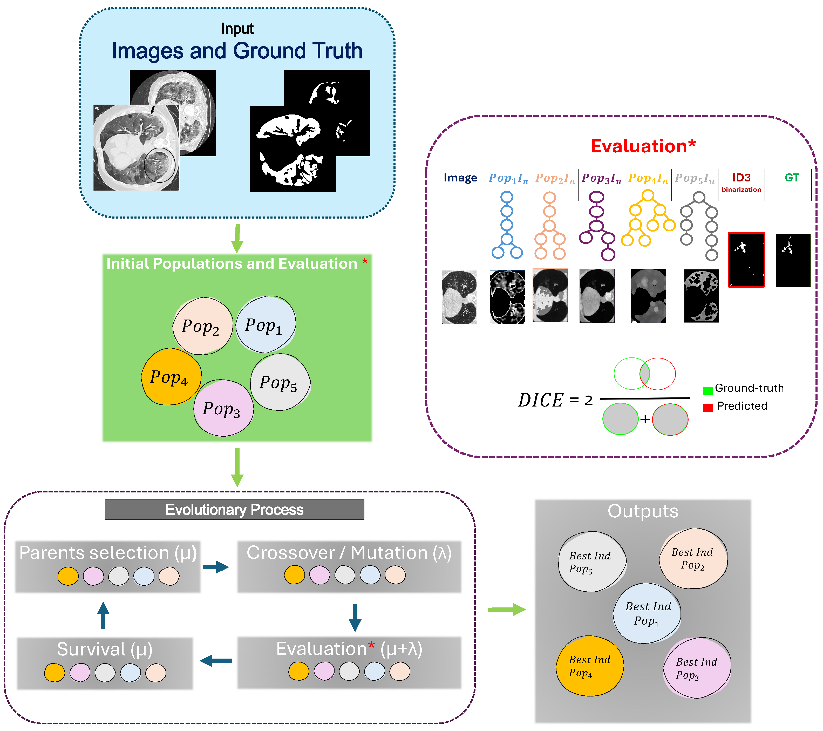
Considering the importance of segmentation tasks within the medical field, our method leverages the tree-based representation of genetic programming, where more than one tree can be generated and evolved to construct and extract more efficient features to perform segmentation tasks. Additionally, our method addresses the segmentation task as a form of pixel classification. In this way, a classifier is used instead of classical techniques such as Otsu or threshold binarization methods. To perform the segmentation, it is necessary to work with the original image and the image already segmented by an expert, also known as Ground Truth (G.T.).

In this manner, we can asses the performance of each individual at the binarization/segmentation step. The proposal uses a wrapper method where the learning algorithm’s performance is used as the evaluation criterion.

Typically, the evolution process involves only one population to evolve. The result from the evolution returns only one individual with the highest fitness according to the metric used during evaluation.

Our method evolves simultaneously and in isolation into five populations. Each population returns one pipeline containing the necessary functions for the feature extraction/construction of the raw grayscale images. These five features are fed into the classifier to perform the pixel classification. Each featured image is converted to a column vector to match the pixel label for the ROI in the G.T. Figure 1 shows the framework of the segmentation based on the features constructed by GP.

First, the data used contain the original images in grayscale. Then, the evolution process includes five populations. The five initial populations are generated using the Full method [22]. This method randomly produces individuals with the same depth in all branches. Then, the five populations are evaluated as if they were one population. For each population, one individual is taken and performs the feature construction/extraction in the images. Then, after processing the images with the functions for each individual, they are converted into a feature vector, where each pixel has its own label.

At this stage, six features are considered for the classifier model. The first is the original grayscale image, and the rest correspond to each feature constructed for each individual selected from the five populations.

The fitness of those individuals is shared among them, i.e, individual 1 in population one shares the same fitness as individual 1 in the other populations.

At this point, the way they are paired for the evaluation and fitness sharing is based on the index of the initial population. The order across populations during the evolution is static, meaning that the individuals keep the same index and remain consistent across generations.

The variation operators, such as crossover and mutation, are performed internally in each population. The $\mu +\lambda$ strategy is adopted into our approach. $\mu$ represents the number of individuals to select for the next generation during the evolutionary process, while $\lambda$ is the number of offspring to generate each generation. This ensures that at the time of evaluation, the offspring for the five populations will be the same number of new individuals.

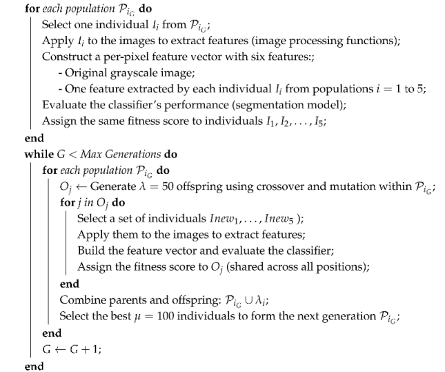
The final result of the evolutionary process is the best individual for each population. The five individuals contain the set of functions of image processing that help the classifier to perform the segmentation. The GP-MIFC pseudocode is shown in Algorithm 1.    

Algorithm 1 GP-MIFC algorithm

Input: Grayscale images

Output: Five individuals, one from each population, with image processing

functions for segmentation

$G\leftarrow 0$

$P_{i_G}\leftarrow$ Initialize five populations ${\mathcal{P}}_1,{\mathcal{P}}_2,\dots ,{\mathcal{P}}_5$ using the Full method by

Koza [22], each with $\mu =100$ individuals

Select the best individual from each population as the final result

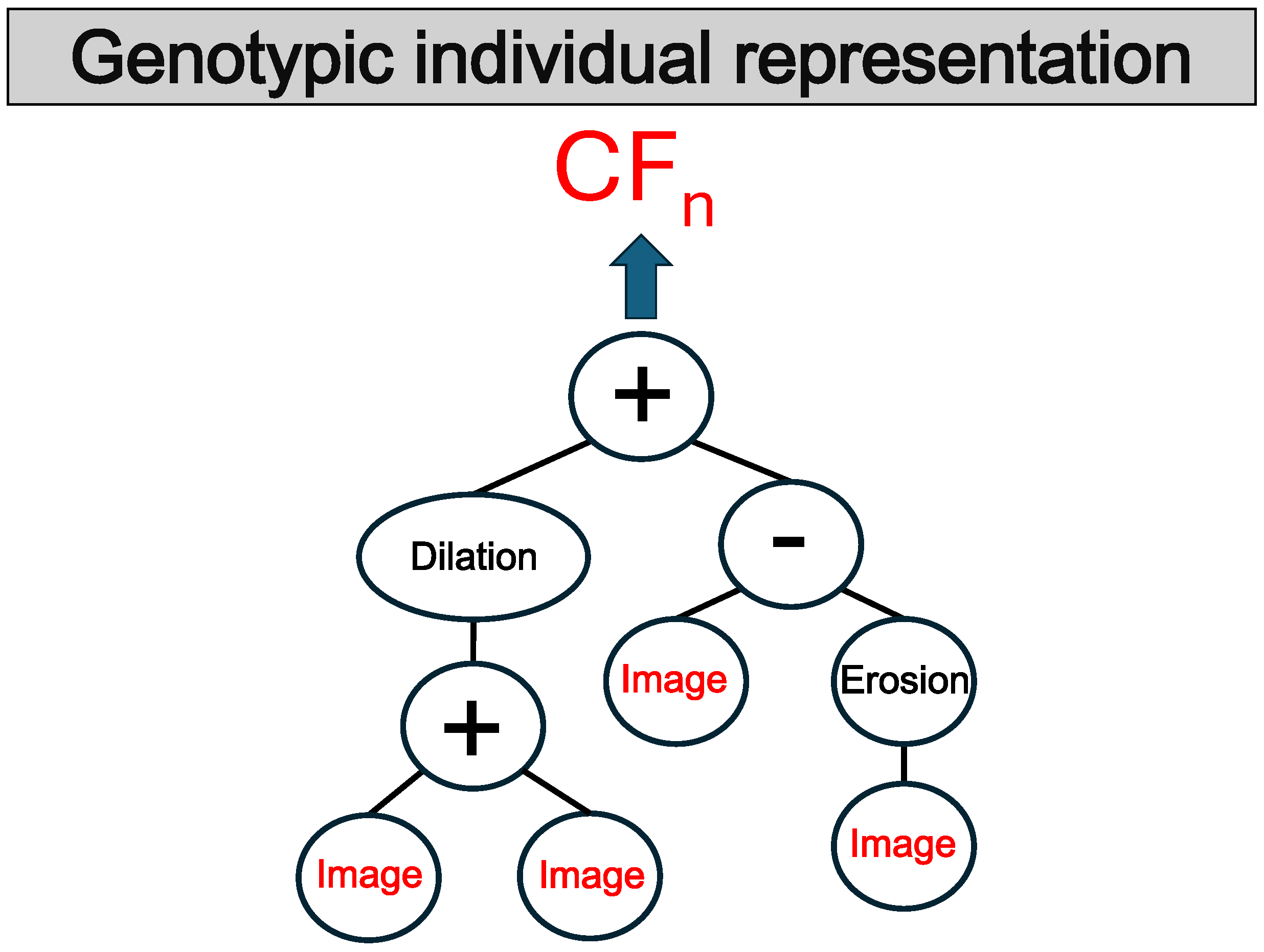
3.1. Representation

As mentioned earlier, the representation used throughout our proposal is trees and five populations within the evolutionary process. The tree-based representation of individuals contains functions, and the leaf nodes involve the variables, which correspond to grayscale images. We use this representation because of its ability to efficiently perform the co-evolution. Also, it is easy to interpret and replicate the pipeline of image processing functions.

Figure 2 shows the individual tree representation.

3.2. Function and Terminal Set

The set of functions used in GP-MIFC is listed in

Table 1. Function set and terminal definitions used in the Genetic Programming framework.

Function	Definition
Addition	Pixel-wise summation: $I(x,y)+I(x,y)$. Useful for combining two images.
Subtraction	Pixel-wise difference: $I(x,y)-I(x,y)$. Highlights contrast.
Erosion	Morphological operation that removes pixels on object boundaries.
Dilation	Morphological operation that adds pixels to object boundaries.
Opening	Erosion followed by dilation, removes small objects/noise.
Closing	Dilation followed by erosion, fills small holes.
Mask (from [8])	Thresholding function: sets pixel to 0 if $I(x,y)<$ threshold.
Gaussian Filter	Smoothes the image using a Gaussian kernel to reduce noise.
Canny Edge Detector	Detects edges based on gradient magnitude.
Gabor Filter	Detects texture patterns using sinusoidal functions modulated by Gaussian.
Invert Values	Transforms intensity: $|255-I(x,y\left)\right|$ to highlight complementary features.
Terminal Set
Grayscale Image (Im)	Input 2D grayscale image used as the terminal node in the tree.

. The function set is divided into pixel, filter, and morphological operation, as suggested in [8].

The pixel operation only considers the pixel value, and the neighborhood is discarded. Each new value depends on the original pixel value in the same position. The new values are calculated following $f\left[I(x,y)\right]\to I^{\prime }(x,y)$. The arithmetic operation functions, such as addition, subtraction, mask [8], and invert values, are used as pixel operations. The addition and subtraction work as a feature construct function. They can mix different features from different filters used in the same image.

The filter functions include the Gaussian and Canny using the default parameters [37]. Gabor filters can take one of five possible frequency values: 0.2, 0.4, 0.6, and 0.8. Likewise, for orientation degrees, one of the following is taken: 15°, 30°, 45°, 75°, and 90°.

Morphological operators included are opening, closing, erosion, and dilation. The structure element employed for operation is a disk using a kernel size of 7 × 7 pixels. It is known that morphological operators work well with grayscale and binary images.

The unique terminal used is called Im. It contains the input for the individual, which is the grayscale image.

3.3. Fitness Function

The proposal focuses on the segmentation task; the most important metric is the DICE coefficient. This metric evaluates the model’s performance on pixel classification in the test set of images and is assigned to individuals. Another reason to use this metric is that it performs well for binary classification and can deal with unbalanced data. Additionally, it is the most common metric used for segmentation. The DICE coefficient is expressed by

$$DICE={\displaystyle \frac{2TP}{2TP+FP+FN}}$$

(1)

where TP is the total of true positives, FN is the total of false negatives, and FP is the total of false positives. The value 0 indicates that the segmentation is poor, and the maximum value of 1 indicates that the segmentation is excellent.

In medical image segmentation, the interpretation of the value of DICE varies according to the images and the difficulty in distinguishing the ROI by humans in different anatomic structures [38]. Typically, working with RMI images and CT, a 0.6 value of the metric DICE can be categorized as satisfactory, especially due to the visual features that can be complex and require major effort to segment. Additionally, in sample visualization, comparing the annotation by the expert with the prediction by the segmentation allows for avoiding a statistical bias [38]. Values higher than 0.7 of DICE can be categorized as good and excellent segmentation, respectively.

Supporting the above, suppose that the ROI of the image covers 100 pixels (G.T.) and the result of the segmentation gives the following values for TP = 50 (pixels correctly segmented), FP = 50 (pixels wrongly segmented), and FN = 50 (pixels not segmented that belong to the ROI). Applying the metric, the value of DICE is 0.5.

Another segmentation case takes the following values: TP = 50, FP = 0, and FN = 50; additionally, the value of the metric DICE is $\approx 0.67$. In both cases, the TP was 50, which means that 50% of the ROI was correctly segmented. However, it does mean that 50% correctly segmented is equal to 0.5 of the DICE metric.

4. Experimental Design

4.1. Parameter Settings and Experiment Configuration

The number of populations used within the co-evolution process was fixed to 5. The objective was to create five features from the raw images instead of only one from the typical evolution process. Five populations are enough to give the necessary information to the classifier model and cover the search space, whereas only one population does not cover it. Additionally, including more than five populations represents consuming more computational resources. The time to construct a feature was multiplied by the number of populations evolved.

The five populations used the same terminals and function, and the primitives gave the search space. At this point, we could not ensure that the final solutions for each population were completely orthogonal. The same parameters were also applied for the five populations, all listed in

Table 2. Configuration details for the Genetic Programming (GP) setup.

Parameter	Value	Description
Number of generations	100	Total evolutionary iterations.
Population size	100	Number of solutions.
Initialization strategy	Full method	Same depth in each branch
Min/Max tree depth	5–15	Defines the range of depth for the expression trees used in evolution.
Selection strategy	Tournament (size = 5)	Selects the fittest individual among five randomly chosen candidates.
Crossover probability	0.75	Probability of recombining subtrees from two parents during evolution.
Mutation probability	0.25	Probability of randomly modifying a subtree to introduce variation.
Reproduction strategy	($\mu$, $\lambda$) = (100, 50)	Evolutionary strategy where 50 children are created from a parent population of 100.

. In this way, the objective was to explore the search space in different regions, not other search spaces. This is why each population evolved independently, and only the fitness was shared among the individuals according to the initial index. Even though the five populations used the same functions, different regions could be explored by the randomness of the initialization populations and the variation operators applied separately on each population. This allowed each population to explore different regions of the search space.

The parameter settings for each population were set as follows. Considering the number of evolved individuals in preliminary research [8] and based on the performance obtained given the experimentation research, our method also used the same parameters of 100 generations and 100 individuals for each population. The $\mu +\lambda$ values were set to 100 and 50, respectively.

Additionally, the crossover and mutation rates were set to 0.75 and 0.25. The crossover operator was one-point, and mutation was the uniform [22]. The maximum and minimum depths of the initial trees were set to 15 and 5, respectively. The tournament was the selection method with a size of 5 individuals.

The model classifier that performed the segmentation throughout the pixel classification was the ID3 decision tree. The maximum depth was set to 5 to avoid overfitting. As part of the wrapper approach, the datasets were split into training and test sets, 70% and 30%, respectively.

The proposal was implemented in Python 3, using DEAP [39], OpenCV [40], Scikit-image [37], and Scikit-learn [41] libraries. The experimentation was performed on a server with 64 Intel Xeon Silver 4216 2.1 GHz CPU’s, 264 GB of memory, and Linux OS. The GP-MIFC was run 10 times for each dataset due to the limited time available on the server, and each execution took more than 5 h. The executions were carried out in a serial configuration.

4.2. Benchmark Datasets

In this paper, we evaluate the performance of the proposed method using four medical datasets. The datasets were selected according to the objective of dealing with different modalities of medical images, such as C.T., MRI, and digital images from cameras. The first dataset is the COVID-19 dataset [42], which contains the computed tomography of lungs affected by COVID-19 with the corresponding mask. This dataset contains 100 images with the corresponding G.T.

The second and third datasets are DRIVE [43] and ISIC [44], which contain 20 and more than 1200 color images, respectively. Finally, the fourth dataset, Intracranial Hemorrhage (MRI-IH) [45], contains MRI. This dataset includes more than 2000 slices of images of brain MRI; however, only 318 MRI images contain the G.T. For experimentation only, 100 images were used for each dataset, except for DRIVE (it only contains 20 images). In the case of those datasets that contain more than 100 images, the selection was performed randomly with different seeds to ensure a fair comparison with other methods. The reason for using only 100 images was to save computational resources. This configuration and seeds are also used for benchmark methods.

4.3. Benchmark Methods

The proposal was compared with four methods. Two of them are based on Genetic Programming. The first one is StronglyGP, and the second is TwoStageGP, both taken from [26]. StronglyGP highlights using the updated version of GP where the set of functions are typed according to a certain type of data. TwostageGP evolves two subpopulations, where the first one uses grayscale images, which are then binarized, in such a way that the second one employs binary image operators.

On the other hand, the well-known CNN’s U-net [9] and U-net++ [19] were used to compare our method. Each model considered a maximum number of 500 epochs using an early stopping strategy with 10 tolerance epochs to save computational cost, and the learning rate was $1\times {10}^{-4}$.

5. Results and Discussion

This section is divided into two subsections. Section 5.1 refers to the results of the proposed method evaluated in different datasets and briefly discusses the performance achieved. In Section 5.2, we compare our method with SOTA methods in the datasets mentioned above.

5.1. Performance for Each Dataset

Table 3. Performance of GP-MIFC in four datasets.

	DICE Performance in Datasets
Statistic	COVID-19	ISIC	DRIVE	MRI-IH
Best	0.81	0.78	0.74	0.56
Worst	0.71	0.71	0.24	0.31
Mean	0.75	0.75	0.58	0.44
Median	0.74	0.76	0.65	0.43
Std. Dev.	0.02	0.03	0.18	0.09

and Figure 3 show the performance statistics of GP-MIFC corresponding to different datasets. The listed values correspond to the performance in the test set. The dataset where GP-MIFC performs better is in the COVID-19 and DRIVE datasets, achieving median values of more than 0.74 of DICE. The dataset where GP-MIFC performs badly is with MRI-IH, achieving mean and median values lower than 0.35 regarding the DICE metric. The best value of segmentation is for the COVID-19 dataset, with a DICE value of 0.81. On the other hand, the worst proposal performance is in the MRI-IH, with a DICE value of 0.31.

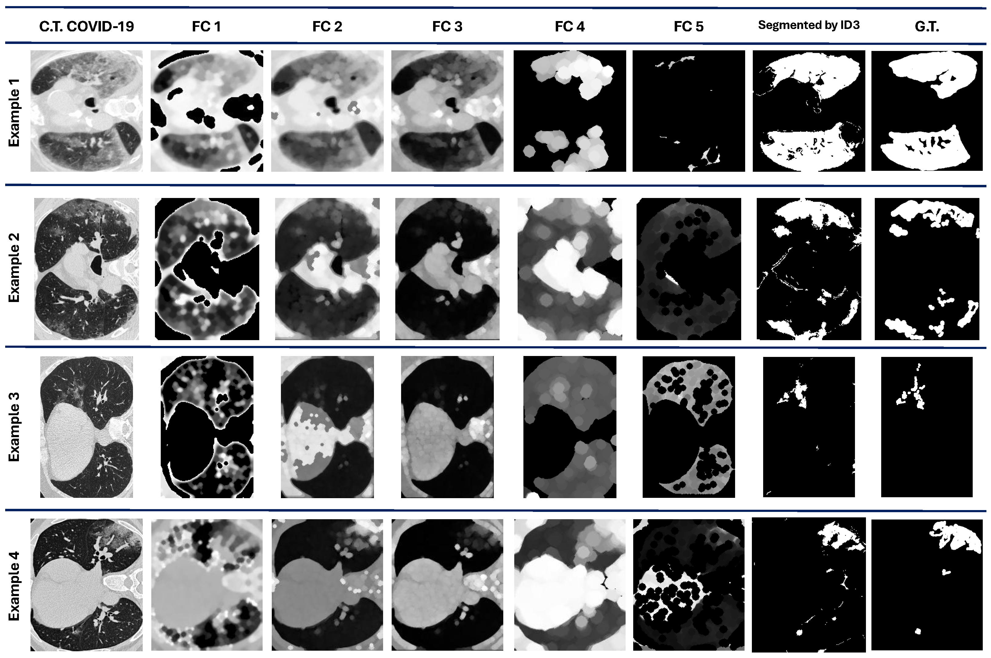
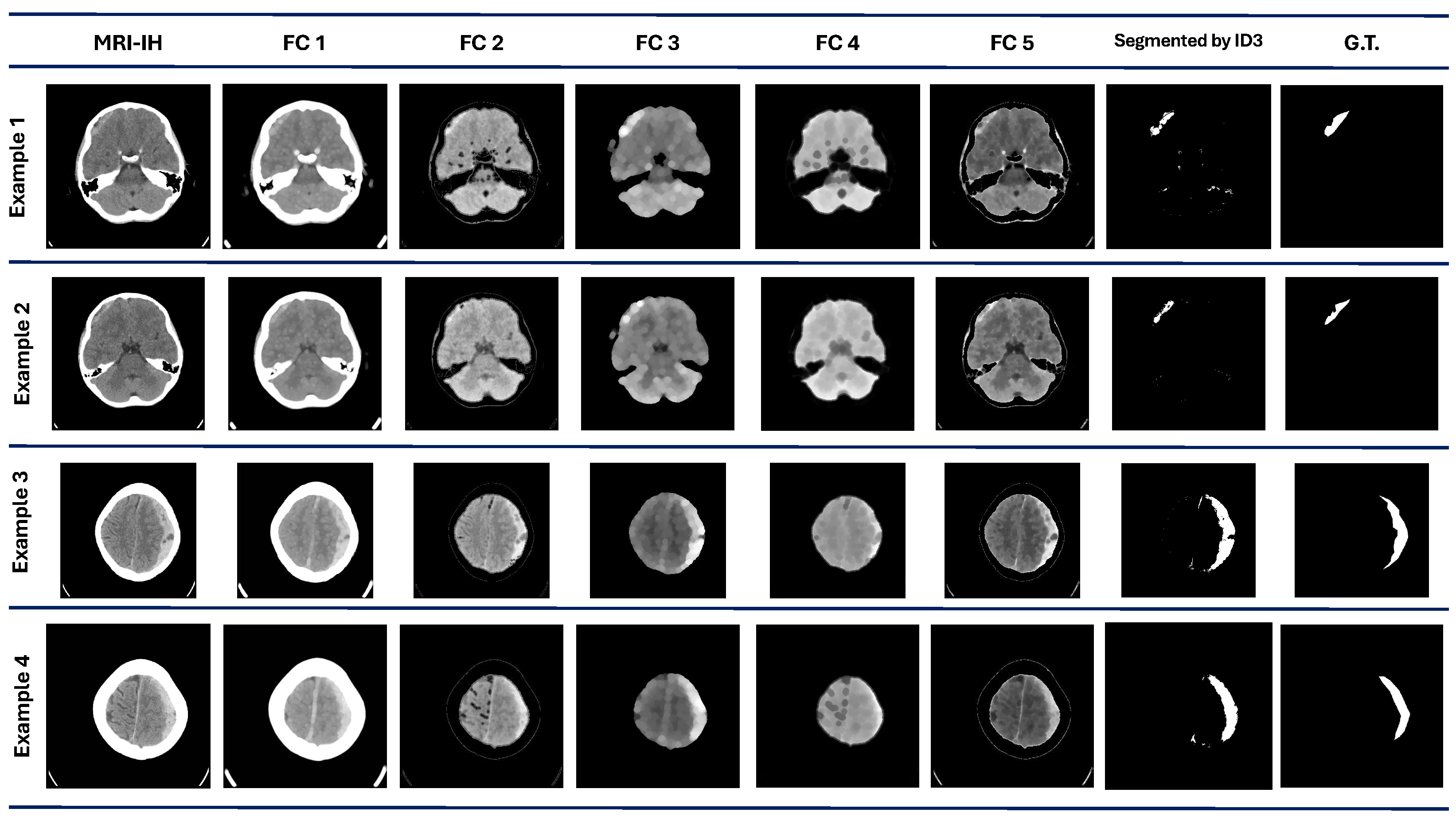
Figure 4 shows four examples of the results obtained from the five best individuals after the evolution process. The original image is also considered a feature for the pixel classification made by the ID3. $F{C}_1,F{C}_2,F{C}_3,F{C}_4$, and $F{C}_5$ are the image features constructed/extracted according to the individual, which contains the pipeline for the image processing.

We can observe that comparing qualitative results in Figure 4 with the quantitative performance with DICE in Table 3 demonstrates that the ROI is marked successfully in some cases, such as in examples 1 and 3. However, in examples 2 and 4, some regions are also marked as ROI even though they are not.

For the performance of the ISIC dataset, the best DICE value achieved is 0.78, and the worst is around 0.72. However, according to the DICE metric, the mean and median are greater than 0.76. The standard deviation demonstrates that the GP-MIFC performs more stably with COVID-19, MRI-IH, and ISIC datasets. Two datasets correspond to C.T. and MRI sources, where, naturally, the images are in grayscale. However, in the ISIC dataset, the algorithm is also stable. The algorithm works without outliers with images originally in grayscale, such as the MRI-IH dataset. It is well known that moving from RGB colors to grayscale results in information loss. As mentioned in [1], the color gives more information as part of the features related to the image content. Surprisingly, the RGB DRIVE dataset achieves values that are higher than 0.65, but it also shows a higher standard deviation than in the grayscale datasets.

For the DRIVE dataset, the mean and median are 0.58 and 0.65, respectively, and the best and worst values obtained are 0.747 and 0.24, respectively. This dataset’s mean and median results are higher than the MRI-IH dataset.

Finally, in the MRI-IH, the algorithm performance achieves a mean and median value of 0.44 and 0.43, respectively. This dataset was the most challenging part of the proposal. The best value achieved is the lowest compared to the other datasets, with only a 0.56 DICE value. Also, it has the second-lowest value for the worst performance in the different datasets. The visual results with this dataset are shown in Figure 5. In example 1, the segmentation results show some regions marked as ROI, according to the G.T. Examples 3 and 4 show a good visual performance. However, some regions are discarded and include areas that do not correspond to the ROI.

The variability among the segmentations by the model and the G.T. given by an expert can be high, mainly due to human bias. This can be attributed to the fact that human segmentations may be influenced by the expert’s experience with a specific imaging modality and their individual visual perception. The variability is present in both cases, in humans and computer programs. The results demonstrate that the variability of our method is present in different percentages according to the dataset.

The significant variability is present in the DRIVE dataset, where some outliers exist and correspond to the worst and lowest values. As we can observe in Figure 3, the MRI-IH dataset reflects the difficulty for our method to perform the segmentation, where the ROIs are small regions that are hard to segment.

Regarding ISIC and COVID-19 datasets, the distribution is lower. However, the COVID-19 dataset has some outliers.

Figure 3 demonstrates the variability, which is highly related to the image complexity of each dataset.

5.2. Comparison with Benchmark Methods

Given the results obtained regarding segmentation quality, a comparison was made between the proposed algorithm and other state-of-the-art methods designed for image segmentation. Two of these methods follow the genetic programming approach, both taken from [26]: StronglyGP and TwostageGP. These were considered in the comparison due to their recent development and the fact that they were tested on various image datasets, obtaining competitive results. It is worth noting that both algorithms were configured using the parameters reported in [26].

On the other hand, the comparison also includes two well-known methods used for medical image segmentation: the convolutional neural networks U-Net [9] and U-Net++ [19].

Table 4. Comparison with benchmark methods for each dataset. The values reported correspond to the medians of ten executions.

Dataset	Method	DICE	SPC/SEN	HD
COVID-19	GP-MIFC	0.74 ↑	0.95/0.80	7.90
	StronglyGP	0.40	0.96/0.33	2045.26
	TwostageGP	0.45	0.89/0.48	16,233.66
	Unet	0.43	0.91/0.63	2300.48
	Unet++	0.54	0.95/0.71	2091.99
ISIC	GP-MIFC	0.76 ↑	0.90/0.85	126.39
	StronglyGP	0.23	0.63/0.19	1680.96
	TwostageGP	0.45	0.81/0.40	1851.13
	Unet	0.19	0.78/0.27	948.09
	Unet++	0.32	0.90/0.34	2157.25
DRIVE	GP-MIFC	0.65 ↑	0.95/0.87	9.01
	StronglyGP	0.54	0.93/0.53	2087.34
	TwostageGP	0.44	0.96/0.31	2697.37
	Unet	0.10	0.91/0.51	1152.01
	Unet++	0.15	0.91/0.66	980.59
MRI-IH	GP-MIFC	0.43 ↑	0.99/0.81	3.93
	StronglyGP	0.13	0.99/0.07	2650.29
	TwostageGP	0.16	0.98/0.11	2542.92
	Unet	0.10	0.99/0.05	2337.89
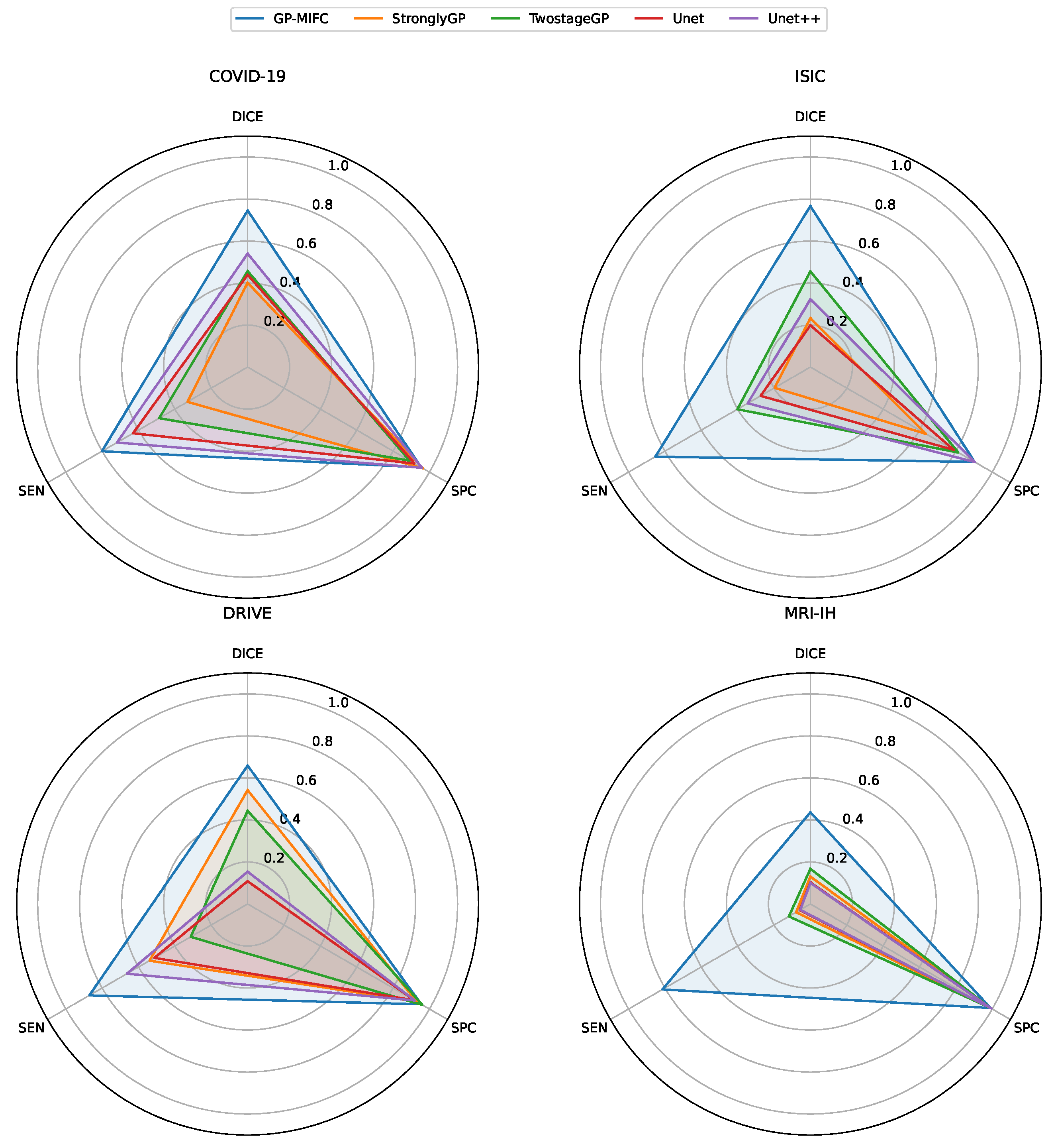
	Unet++	0.10	0.99/0.05	2396.68

reports the median values for each method compared. Each method was executed 10 times. The values marked with ↑ for only the DICE metric indicate the best result, according to the Mann–Whitney U statistical test with a 95% confidence level. The results for the metrics specificity (SPC), sensitivity (SEN), and Hausdorff Distance are also reported in detail. The highest median values for each method and metric are highlighted in bold.

Figure 6 contains a radar chart for each dataset, where the benchmark methods are compared with our method GP-MIFC in terms of DICE, specificity, and sensitivity metrics.

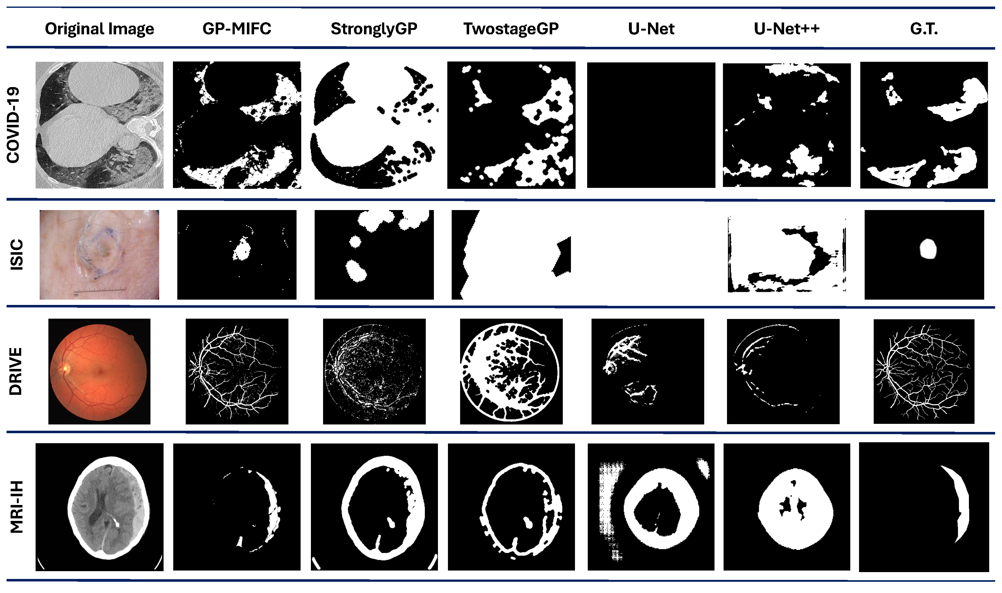
For the first dataset containing COVID-19 images, GP-MIFC showed favorable results regarding segmentation performance. As seen in Table 4, the values achieved are outstanding compared to the other methods. Regarding StronglyGP, its performance was not favorable due to its use of Otsu’s method for binarization, which led to less competitive segmentation in a portion of the images. In contrast, TwostageGP achieved better performance than StronglyGP.

The performance of the CNNs is also noteworthy, with UNet++ reaching a value of 0.54038. UNet++ outperformed UNet, TwostageGP, and StronglyGP, but not GP-MIFC. Visually, the results do not clearly show the affected lung area, as some final images appear completely dark.

The proposed algorithm significantly outperformed the other algorithms in the ISIC dataset. The second-best performance was obtained by TwostageGP, which benefits from applying certain operations and filters in the first stage and then processing the already-binarized image in the second stage. The performance of UNet and UNet++ was unfavorable; although some of the resulting images visually resemble the target image, the DICE metric indicates otherwise.

The third dataset used for comparison is DRIVE. For GP-MIFC, both visual- and segmentation-level performances were favorable. The method achieved a DICE score above 0.60, surpassing the other methods. Interestingly, the genetic programming-based methods performed more competitively than the CNNs. For this dataset, StronglyGP outperformed TwostageGP. The CNNs showed poor segmentation performance and visual interpretation of the resulting images.

Lastly, none of the comparison methods reached a DICE value of 0.2 for the MRI-IH dataset. Even GP-MIFC did not perform as well on the other datasets. Moreover, due to the nature of the images, accurately identifying the hemorrhage area is challenging, as it represents a very small portion of the entire image. Despite this challenge, GP-MIFC still achieved a meaningful level of performance compared to the other methods, with some resulting images clearly showing the area of interest. This was not the case for the other methods, which failed to approach the target image.

Based on the results and comparisons between all methods, it is evident that the proposed GP-MIFC algorithm performs competitively compared to state-of-the-art methods. Additionally, the visual perception of the resulting images allows for the easy identification of the area of interest, making this tool capable of constructing the necessary features to perform accurate segmentation. Figure 7 shows the comparison results with benchmark methods in the four datasets.

6. Conclusions

Based on the results obtained in this work, it is clear that the capability of evolutionary algorithms can achieve competitive results. Although they do not guarantee finding the optimal solution, they offer one or more solutions that can effectively address the problem. In this work, genetic programming provided the opportunity to create solutions using programs and image processing functions to perform the feature construction process, enabling adequate segmentation of the ROI and demonstrating competitiveness compared to various current algorithms that tackle the segmentation problem.

In this work, the design of the GP-MIFC algorithm, which performs automatic feature construction to achieve competitive segmentation and identify the ROI in the images, was presented. The proposed method achieved competitive values, with segmentation performance exceeding 0.7 regarding the DICE metric. Moreover, the ROI was identified clearly and concisely.

With the obtained results, comparisons were made with other SOTA methods that perform the image segmentation task. Two of them were based on genetic programming, and the remaining two were based on convolutional neural networks.

Part of our future work is to use the updated version of GP, Strongly Genetic Programming, to include the classifiers within the individual. Additionally, strategies such as surrogate models or inheritance can speed up the image processing during individual evaluation since the evolutionary process takes a long time. It is important to consider reducing the computational cost without affecting the segmentation performance. Future research would be appropriate to explore changing the search space for each population, modifying the primitive set for each, and using different parameters for the variation operators to ensure orthogonality across the final co-evolution solutions.

References

- Herrera-Sánchez, D.; Acosta-Mesa, H.G.; Mezura-Montes, E.; Márquez-Grajales, A. Shifting Color Space for Image Classification using Genetic Programming. In Proceedings of the GECCO 2024 Companion—Proceedings of the 2024 Genetic and Evolutionary Computation Conference Companion, Melbourne, VIC, Australia, 14–18 July 2024; pp. 283–286. [Google Scholar] [CrossRef]
- Ling, Y.; Wang, Y.; Dai, W.; Yu, J.; Liang, P.; Kong, D. MTANet: Multi-Task Attention Network for Automatic Medical Image Segmentation and Classification. IEEE Trans. Med. Imaging 2024, 43, 674–685. [Google Scholar] [CrossRef] [PubMed]
- Liu, X.; Song, L.; Liu, S.; Zhang, Y.; Feliu, C.; Burgos, D. A Review of Deep-Learning-Based Medical Image Segmentation Methods. Sustainability 2021, 13, 1224. [Google Scholar] [CrossRef]
- Lensen, A.; Al-Sahaf, H.; Zhang, M.; Xue, B. Genetic Programming for Region Detection, Feature Extraction, Feature Construction and Classification in Image Data. In Genetic Programming. EuroGP 2016. Lecture Notes in Computer Science; Springer: Cham, Switzerland, 2016; Volume 9594, pp. 51–67. [Google Scholar] [CrossRef]
- Bi, Y.; Xue, B.; Zhang, M. Dual-Tree Genetic Programming for Few-Shot Image Classification. IEEE Trans. Evol. Comput. 2022, 26, 555–569. [Google Scholar] [CrossRef]
- Sun, Y.; Zhang, Z. Automatic Feature Construction-Based Genetic Programming for Degraded Image Classification. Appl. Sci. 2024, 14, 1613. [Google Scholar] [CrossRef]
- Fuentes-Tomás, J.A.; Mezura-Montes, E.; Acosta-Mesa, H.G.; Márquez-Grajales, A. Tree-Based Codification in Neural Architecture Search for Medical Image Segmentation. IEEE Trans. Evol. Comput. 2024, 28, 597–607. [Google Scholar] [CrossRef]
- Herrera-Sánchez, D.; Fuentes-Tomás, J.A.; Acosta-Mesa, H.G.; Mezura-Montes, E. Experimental Study for Automatic Feature Construction to Segment Images of Lungs Affected by COVID-19 Using Genetic Programming. Lect. Notes Comput. Sci. 2025, 15465 LNAI, 155–166. [Google Scholar] [CrossRef]
- Ronneberger, O.; Fischer, P.; Brox, T. U-Net: Convolutional Networks for Biomedical Image Segmentation. In Medical Image Computing and Computer-Assisted Intervention—MICCAI 2015. MICCAI 2015. Lecture Notes in Computer Science; Springer: Cham, Switzerland, 2015; Volume 9351, pp. 234–241. [Google Scholar] [CrossRef]
- Cai, Y.; Yuan, J. A Review of U-Net Network Medical Image Segmentation Applications. In Proceedings of the 2022 5th International Conference on Artificial Intelligence and Pattern Recognition (AIPR ’22), Xiamen, China, 23–25 September 2022; pp. 457–461. [Google Scholar] [CrossRef]
- Naser, M.A.; Deen, M.J. Brain tumor segmentation and grading of lower-grade glioma using deep learning in MRI images. Comput. Biol. Med. 2020, 121, 103758. [Google Scholar] [CrossRef]
- Liang, Y.; Zhang, M.; Browne, W.N. Image Segmentation: A Survey of Methods Based on Evolutionary Computation. In Simulated Evolution and Learning. SEAL 2014. Lecture Notes in Computer Science; Springer: Cham, Switzerland, 2014; Volume 8886, pp. 847–859. [Google Scholar] [CrossRef]
- Herrera-Sánchez, D.; Acosta-Mesa, H.G.; Mezura-Montes, E.; Herrera-Meza, S.; Rivadeneyra-Domínguez, E.; Zamora-Bello, I.; Almanza-Domínguez, M.F. Imaging Estimation for Liver Damage Using Automated Approach Based on Genetic Programming. Math. Comput. Appl. 2025, 30, 25. [Google Scholar] [CrossRef]
- Miller, C.G.; Krasnow, J.; Schwartz, L.H. Medical imaging in clinical trials. In Medical Imaging in Clinical Trials; Springer: London, UK, 2013; pp. 1–420. ISBN 9781848827103. [Google Scholar] [CrossRef]
- Mahesh, M. The Essential Physics of Medical Imaging. Med. Phys. 2013, 40, 077301. [Google Scholar] [CrossRef]
- Guo, Y.; Nie, G.; Gao, W.; Liao, M. 2D Semantic Segmentation: Recent Developments and Future Directions. Future Internet 2023, 15, 205. [Google Scholar] [CrossRef]
- Liu, S.; Qi, L.; Qin, H.; Shi, J.; Jia, J. Path Aggregation Network for Instance Segmentation. In Proceedings of the IEEE Computer Society Conference on Computer Vision and Pattern Recognition, Salt Lake City, UT, USA, 18–23 June 2018; pp. 8759–8768. [Google Scholar] [CrossRef]
- Kirillov, A.; He, K.; Girshick, R.; Rother, C.; Dollar, P. Panoptic segmentation. In Proceedings of the IEEE Computer Society Conference on Computer Vision and Pattern Recognition, Long Beach, CA, USA, 15–20 June 2019; pp. 9396–9405. [Google Scholar] [CrossRef]
- Zhou, Z.; Rahman Siddiquee, M.M.; Tajbakhsh, N.; Liang, J. Unet++: A nested u-net architecture for medical image segmentation. In Lecture Notes in Computer Science (Including Subseries Lecture Notes in Artificial Intelligence and Lecture Notes in Bioinformatics); Springer International Publishing: Berlin/Heidelberg, Germany, 2018; Volume 11045 LNCS, pp. 3–11. [Google Scholar] [CrossRef]
- Mei, Y.; Chen, Q.; Lensen, A.; Xue, B.; Zhang, M. Explainable Artificial Intelligence by Genetic Programming: A Survey. IEEE Trans. Evol. Comput. 2023, 27, 621–641. [Google Scholar] [CrossRef]
- Quinlan, J.R. Induction of decision trees. Mach. Learn. 1986, 1, 81–106. [Google Scholar] [CrossRef]
- Koza, J.R. Genetic Programming On the Programming of Computers by Means of Natural Selection. Stat. Comput. 1994, 4, 87–112. [Google Scholar] [CrossRef]
- Miller, J.F. Cartesian Genetic Programming. In Cartesian Genetic Programming; Springer: Berlin/Heidelberg, Germany, 2011; pp. 17–34. [Google Scholar] [CrossRef]
- Mckay, R.I.; Hoai, N.X.; Whigham, P.A.; Shan, Y.; O’Neill, M. Grammar-based Genetic Programming: A survey. Genet. Program. Evolvable Mach. 2010, 11, 365–396. [Google Scholar] [CrossRef]
- Brameier, M.F.; Banzhaf, W. Linear Genetic Programming. In Linear Genetic Programming; Springer: Berlin/Heidelberg, Germany, 2007. [Google Scholar] [CrossRef]
- Liang, J.; Wen, J.; Wang, Z.; Wang, J. Evolving semantic object segmentation methods automatically by genetic programming from images and image processing operators. Soft Comput. 2020, 24, 12887–12900. [Google Scholar] [CrossRef]
- Liang, Y.; Zhang, M.; Browne, W.N. Image feature selection using genetic programming for figure-ground segmentation. Eng. Appl. Artif. Intell. 2017, 62, 96–108. [Google Scholar] [CrossRef]
- Liang, Y.; Zhang, M.; Browne, W.N. Figure-ground image segmentation using feature-based multi-objective genetic programming techniques. Neural Comput. Appl. 2019, 31, 3075–3094. [Google Scholar] [CrossRef]
- Mahmood, M.T. Defocus Blur Segmentation Using Genetic Programming and Adaptive Threshold. Comput. Mater. Contin. 2021, 70, 4867–4882. [Google Scholar] [CrossRef]
- Yuan, D.; Zhang, D.; Yang, Y.; Yang, S. Automatic construction of filter tree by genetic programming for ultrasound guidance image segmentation. Biomed. Signal Process. Control 2022, 76, 103641. [Google Scholar] [CrossRef]
- Correia, J.; Rodriguez-Fernandez, N.; Vieira, L.; Romero, J.; Machado, P. Towards Automatic Image Enhancement with Genetic Programming and Machine Learning. Appl. Sci. 2022, 12, 2212. [Google Scholar] [CrossRef]
- Ingalalli, V.; Silva, S.; Castelli, M.; Vanneschi, L. A Multi-dimensional Genetic Programming Approach for Multi-class Classification Problems. In Genetic Programming. EuroGP 2014. Lecture Notes in Computer Science; Springer: Berlin/Heidelberg, Germany, 2014; Volume 8599, pp. 48–60. [Google Scholar] [CrossRef]
- Muñoz, L.; Silva, S.; Trujillo, L. M3GP—Multiclass Classification with GP. In Genetic Programming. EuroGP 2015. Lecture Notes in Computer Science; Springer: Cham, Switzerland, 2015; Volume 9025, pp. 78–91. [Google Scholar] [CrossRef]
- La Cava, W.; Silva, S.; Vanneschi, L.; Spector, L.; Moore, J. Genetic Programming Representations for Multi-dimensional Feature Learning in Biomedical Classification. In Applications of Evolutionary Computation. EvoApplications 2017. Lecture Notes in Computer Science); Springer: Cham, Switzerland, 2017; Volume 10199 LNCS, pp. 158–173. [Google Scholar] [CrossRef]
- Cárdenas Florido, L.; Trujillo, L.; Hernandez, D.E.; Muñoz Contreras, J.M. M5GP: Parallel Multidimensional Genetic Programming with Multidimensional Populations for Symbolic Regression. Math. Comput. Appl. 2024, 29, 25. [Google Scholar] [CrossRef]
- Batista, J.E.; Rodrigues, N.M.; Vanneschi, L.; Silva, S. M6GP: Multiobjective Feature Engineering. In Proceedings of the 2024 IEEE Congress on Evolutionary Computation, CEC 2024—Proceedings, Yokohama, Japan, 30 June–5 July 2024. [Google Scholar] [CrossRef]
- Van Der Walt, S.; Schönberger, J.L.; Nunez-Iglesias, J.; Boulogne, F.; Warner, J.D.; Yager, N.; Gouillart, E.; Yu, T. Scikit-image: Image processing in python. PeerJ 2014, 2014, e453. [Google Scholar] [CrossRef] [PubMed]
- Müller, D.; Soto-Rey, I.; Kramer, F. Towards a guideline for evaluation metrics in medical image segmentation. BMC Res. Notes 2022, 15, 210. [Google Scholar] [CrossRef]
- Kim, J.; Yoo, S. Software review: DEAP (Distributed Evolutionary Algorithm in Python) library. Genet. Program. Evolvable Mach. 2019, 20, 139–142. [Google Scholar] [CrossRef]
- Bradski, G. The OpenCV Library. Dr. Dobb’s J. Softw. Tools 2000, 25, 120–123. [Google Scholar]
- Pedregosa, F.; Varoquaux, G.; Gramfort, A.; Michel, V.; Thirion, B.; Grisel, O.; Blondel, M.; Prettenhofer, P.; Weiss, R.; Dubourg, V.; et al. Scikit-learn: Machine learning in Python. J. Mach. Learn. Res. 2011, 12, 2825–2830. [Google Scholar]
- MedSeg; Jenssen, H.B.; Sakinis, T. MedSeg Covid Dataset 1. Available online: https://doi.org/10.6084/m9.figshare.13521488.v2 (accessed on 16 April 2025).
- Staal, J.; Abràmoff, M.D.; Niemeijer, M.; Viergever, M.A.; Van Ginneken, B. Ridge-based vessel segmentation in color images of the retina. IEEE Trans. Med. Imaging 2004, 23, 501–509. [Google Scholar] [CrossRef]
- Gutman, D.; Codella, N.C.F.; Celebi, E.; Helba, B.; Marchetti, M.; Mishra, N.; Halpern, A. Skin Lesion Analysis toward Melanoma Detection: A Challenge at the International Symposium on Biomedical Imaging (ISBI) 2016, hosted by the International Skin Imaging Collaboration (ISIC). arXiv 2016, arXiv:1605.01397. [Google Scholar]
- Hssayeni, M.D.; Croock, M.S.; Salman, A.D.; Al-Khafaji, H.F.; Yahya, Z.A.; Ghoraani, B. Intracranial Hemorrhage Segmentation Using a Deep Convolutional Model. Data 2020, 5, 14. [Google Scholar] [CrossRef]