Comparative Analysis of ALE Method Implementation in Time Integration Schemes for Pile Penetration Modeling

Abstract

This study investigates the full penetration simulation of piles from the ground surface, focusing on frictional contact modeling without mesh distortion. To overcome issues related to mesh distortion and improve solution convergence, the Arbitrary Lagrangian–Eulerian (ALE) adaptive mesh technique was implemented within both explicit and implicit time integration schemes. The numerical model was validated against field experiments conducted at Bothkennar, Scotland, using the Imperial College instrumented displacement pile (ICP) in soft clay, where the soil behavior was effectively represented using the modified Cam-Clay model and the Mohr–Coulomb model. The primary objectives of this study are to evaluate the ALE method performance in handling mesh distortion; analyze the effects of soil–pile interface friction, pile dimensions, and various dilation angles on pile resistance; and compare the effectiveness of explicit and implicit time integration schemes in terms of stability, computational efficiency, and solution accuracy. The ALE method effectively modeled pile penetration in Bothkennar clay, validating the numerical model against field experiments. Comparative analysis revealed the explicit time integration method as more robust and computationally efficient, particularly for complex soil–pile interactions with higher friction coefficients.

1. Introduction

Pile foundations are commonly used to support structures on soft soils. Load transfer between pile and soil occurs primarily through frictional contact at the interface. Significant soil deformations and sliding can occur at this interface during pile installation [1,2,3,4].

The calibration chamber model pile [5,6,7] and field experiments [8,9,10,11,12,13,14,15] yielded satisfactory outcomes in terms of the stress and strain distributions induced during installation in soil. These empirical findings demonstrate a superior predictive capacity compared to theoretical solutions, which fail to adequately forecast such an installation process. Owing to the constrained quantity of sensors positioned in proximity to the pile shaft, stress and strain data are confined to discrete regions, rendering it challenging to experimentally acquire comprehensive, large-scale assessments of the soil characteristics enveloping the pile. Consequently, computational techniques can yield precise and economically viable resolutions to these challenges, thereby enhancing the analysis of experimental outcomes and improving the precision of stress and strain distribution estimations [16].

The process of installing piles into the ground can significantly deform the surrounding soil caused by frictional contact and large deformation, which can negatively impact the accuracy of finite element models. To address this issue, researchers have employed numerical methods like the Coupled Eulerian–Lagrangian (CEL) method [17,18,19,20,21,22] and the Arbitrary Lagrangian–Eulerian (ALE) method [23,24,25,26], as well as the Material Point Method (MPM) [27,28]. These methods have been demonstrated to be effective in mitigating the challenges associated with large deformations during pile installation.

Traditional finite element methods using Lagrangian formulations often struggle with severe mesh distortion during pile penetration simulation, leading to numerical instabilities and solution divergence [29]. The Arbitrary Lagrangian–Eulerian (ALE) method has emerged as a promising solution to overcome these limitations. Originally developed for fluid dynamics applications [30], the ALE has gained traction in solid mechanics, particularly in geotechnical applications involving large deformations [31]. The ALE method allows the mesh to move independently of the material, which prevents excessive distortion. This is achieved by defining a fixed reference mesh and moving computational meshes. The material is then mapped onto the computational mesh at each time step. ALE-based finite element models have been successfully used to analyze problems involving large deformations in geotechnical engineering.

Although previous studies have demonstrated the potential of the ALE method in geotechnical applications, a comprehensive comparison of its performance across different time integration schemes is still required. The choice between explicit and implicit time integration schemes significantly influences simulation stability, accuracy, and computational efficiency [32,33]. This decision becomes particularly crucial when modeling complex soil–pile interactions involving frictional contact [16,34].

Well-documented field tests, particularly those conducted at Bothkennar, Scotland, using the Imperial College instrumented displacement pile (ICP) in soft clay, have provided valuable data for validating numerical models [35]. These experiments have become a benchmark for evaluating the effectiveness of different numerical approaches in simulating pile installation processes. Notably, Rezania et al. [36] implemented the cavity-expansion method (CEM), while Tan et al. [37] employed a small-strain numerical approach known as the press–replace method (PRM). More recently, Li et al. [38] applied the zipper technique, initially developed by Mabsout and Tassoulas [39]. Nevertheless, across all these studies, a comprehensive simulation of the full penetration of a pile from the ground surface using frictional contact at the interface was not achieved.

The present study aims to bridge existing knowledge gaps by implementing the ALE method to simulate the entire pile penetration process from the ground surface to the target depth. Validation of the numerical models is carried out through comparison with field data derived from a jacked pile test conducted in soft clay at Bothkennar, Scotland. This research includes assessing the effectiveness of the ALE formulation, implemented within both explicit and implicit time integration schemes, in handling mesh distortion. Additionally, it also evaluates the stability, accuracy, and computational efficiency of the integration solutions when modeling pile installation. Furthermore, this study examines the effect of pile dimensions and various dilation angles on pile resistance, as well as the influence of the friction coefficient at the soil–pile interface on the total resistance of a pile.

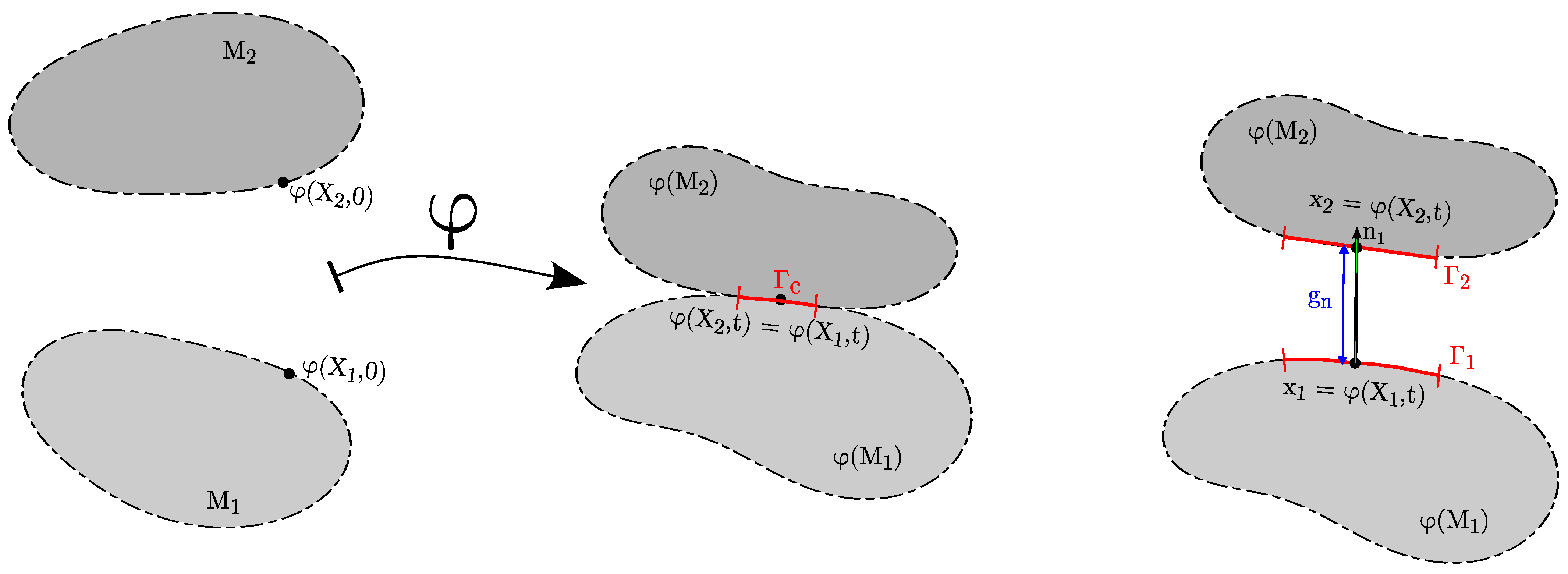
2. Contact Kinematics

Contact kinematics play a key role in the analysis of pile installation processes. Therefore, the basics of the normal and frictional contact constraints used in this work are introduced in this section. Two elastic bodies $M_{\omega }$ ($\omega$ = 1, 2) shown in Figure 1 come into contact, where ${\Gamma }_{\omega }$ is the boundary of a body $M_{\omega }$. $x_{\omega }=\phi (X_{\omega },t)$ indicates the position coordinates at time t in deformed configuration $\phi \left(M_{\omega }\right)$ and $X_{\omega }=\phi (X_{\omega },0)$ denotes the position coordinates of the reference configuration $M_{\omega }$ at time 0, where $u_{\omega }$ is the displacement field:

$$x_{\omega }=X_{\omega }+u_{\omega }$$

(1)

$\phi :M_{\omega }\to \phi \left(M_{\omega }\right)$ is designated as the deformation mapping, which describes the transformation of the body $M_{\omega }$ from its initial configuration to its deformed configuration [40]. Observe in Figure 1 that within the reference configuration, the positions $X_1$ and $X_2$ corresponding to the two distinct material points of bodies $M_1$ and $M_2$, respectively, are capable of coinciding at an identical position $\phi (X_1,t)$ = $\phi (X_2,t)$ in the deformed configuration during the deformation process.

The normal vector $n_1$ corresponds to body $M_1$, while $g_n$ represents the gap or penetration distance between $M_1$ and $M_2$.

$$g_n=(x_2-x_1)·n_1$$

(2)

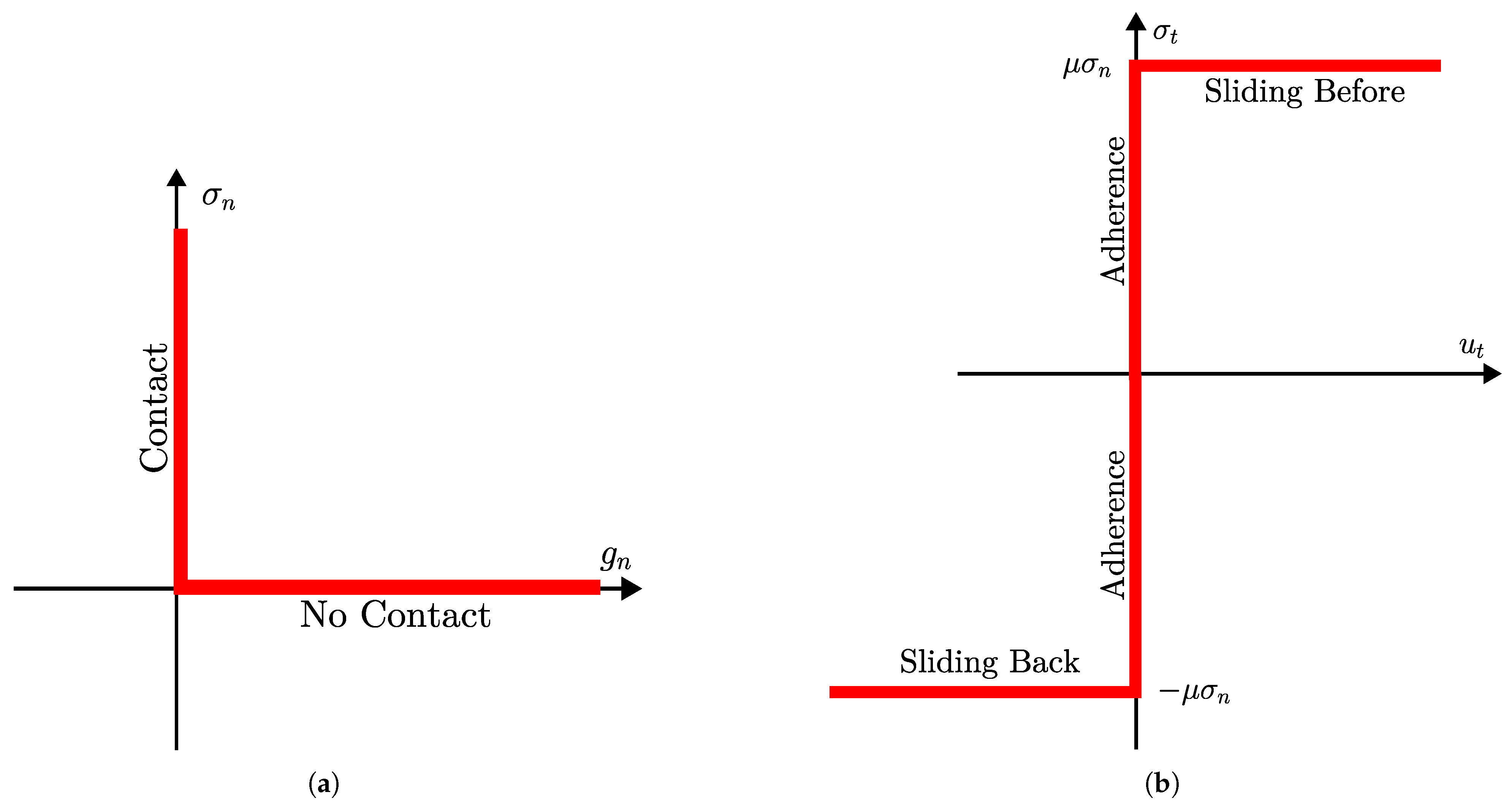
2.1. Normal Conditions

The usual approach for handling normal contact in mechanics is to consider it as a problem of unilateral contact when two solid bodies are in contact. Signorini conditions are used to express unilateral contact in three conditions [41], as illustrated in Figure 2:

$$g_n\ge 0,{\sigma }_n\ge 0,{\sigma }_n·g_n=0$$

(3)

• No penetration occurs                   $g_n\ge 0$
• Compressive contact stress           ${\sigma }_n\ge 0$
• The normal contact stress ${\sigma }_n$ exists only when the surfaces are in contact ($g_n=0$) and ${\sigma }_n=0$ when the surfaces are separated ($g_n>0$). These complementary conditions are formulated as ${\sigma }_n·g_n=0$.

2.2. Contact with Friction

The tangential stress at the contact interface can be split into two actions, which can be either negative or positive. In the beginning, force F does not cause any tangential displacement in the region of contact. This behavior is known as adherence; see Figure 2. The next action caused by force F is related to a tangential displacement in the contact interface, representing what is called sliding [41]. The friction law of Coulomb for isotropic contact and friction is written as follows:

• Contact with adherence

  $$|{\sigma }_t|<\mu {\sigma }_n\mathrm{and}{u}_t=0$$

  (4)
• Contact with slip

  $$|{\sigma }_t|=\mu {\sigma }_n\mathrm{and}\left|u_t\right|>0$$

  (5)

  where $\mu$ is the coefficient of friction, ${\sigma }_t$ and $u_t$, respectively, are the tangential contact stress and the tangential displacement.

3. Numerical Methods

3.1. Numerical Time Integration Schemes

The choice between explicit and implicit time integration schemes plays a crucial role in solving dynamic problems. The general equation of motion is given by the following:

$$\mathbf{M}\ddot{\mathbf{u}}+\mathbf{C}\dot{\mathbf{u}}+\mathbf{K}\mathbf{u}=\mathbf{F}\left(t\right)$$

(6)

At a discrete time $t_{n+1}=t_n+\mathsf{\Delta }t$, Equation (6) can be written as

$$\mathbf{M}{\ddot{\mathbf{u}}}_{n+1}+\mathbf{C}{\dot{\mathbf{u}}}_{n+1}+\mathbf{K}{\mathbf{u}}_{n+1}={\mathbf{F}}_{n+1}$$

(7)

where $\mathbf{M}$ is the mass matrix, $\mathbf{C}$ is the damping matrix, $\mathbf{K}$ is the stiffness matrix, $\mathbf{u}$ is the displacement vector, and $\mathbf{F}\left(t\right)$ is the external force vector. The solution of Equations (6) and (7) by explicit or implicit time integration is discussed in the following.

3.1.1. Explicit Time Integration

The explicit method computes the state at time $t_{n+1}$ directly from the known information at time $t_n$. It does not require solving a system of equations. By using the central difference scheme, the displacement at time step $t_{n+1}$ is given by

$${\mathbf{u}}_{n+1}={\mathbf{u}}_n+\mathsf{\Delta }t{\dot{\mathbf{u}}}_n+{\displaystyle \frac{\mathsf{\Delta }{t}^2}{2}}{\ddot{\mathbf{u}}}_n$$

(8)

The acceleration vector ${\ddot{\mathbf{u}}}_n$ at time $t_n$ is obtained as follows:

$${\ddot{\mathbf{u}}}_n={\mathbf{M}}^{-1}({\mathbf{F}}_n-\mathbf{C}{\dot{\mathbf{u}}}_n-\mathbf{K}{\mathbf{u}}_n)$$

(9)

And at time $t_{n+1}$,

$${\ddot{\mathbf{u}}}_{n+1}={\mathbf{M}}^{-1}({\mathbf{F}}_{n+1}-\mathbf{C}{\dot{\mathbf{u}}}_{n+1}-\mathbf{K}{\mathbf{u}}_{n+1})$$

(10)

The velocity is updated using the average of accelerations at $t_n$ and $t_{n+1}$:

$${\dot{\mathbf{u}}}_{n+1}={\dot{\mathbf{u}}}_n+{\displaystyle \frac{\mathsf{\Delta }t}{2}}({\ddot{\mathbf{u}}}_n+{\ddot{\mathbf{u}}}_{n+1})$$

(11)

The acceleration ${\ddot{\mathbf{u}}}_{n+1}$ is then computed by solving Equation (7) [42]:

$${\ddot{\mathbf{u}}}_{n+1}={\left(\mathbf{M}+{\displaystyle \frac{\mathsf{\Delta }t}{2}}\mathbf{C}\right)}^{-1}\left({\mathbf{F}}_{n+1}-{\displaystyle \frac{\mathsf{\Delta }t}{2}}\mathbf{C}{\ddot{\mathbf{u}}}_n-\mathbf{K}{\mathbf{u}}_{n+1}\right)$$

(12)

The stability condition for explicit schemes is governed by the Courant–Friedrichs–Lewy (CFL) condition:

$$\mathsf{\Delta }t\le \mathsf{\Delta }{t}_{cr}={\displaystyle \frac{L_{min}}{C_d}}$$

(13)

where $L_{min}$ represents the smallest dimension of an element in the mesh, while $C_d$ denotes the dilatational wave speed.

Since no system of equations is solved, the explicit method is computationally efficient for each time step but may require a large number of time steps due to small $\mathsf{\Delta }t$.

3.1.2. Implicit Time Integration

In implicit schemes, such as the Newmark-$\beta$ method [43], the state at time $t_{n+1}$ is obtained by solving a system of equations that considers both the known state at time $t_n$ and the unknowns at time $t_{n+1}$. The displacement and velocity updates are given by the following:

$$\begin{array}{cc}\hfill {\mathbf{u}}_{n+1}& ={\mathbf{u}}_n+\mathsf{\Delta }t{\dot{\mathbf{u}}}_n+{\displaystyle \frac{\mathsf{\Delta }{t}^2}{2}}[(1-2\beta ){\ddot{\mathbf{u}}}_n+2\beta {\ddot{\mathbf{u}}}_{n+1}]\hfill \end{array}$$

(14)

$$\begin{array}{cc}\hfill {\dot{\mathbf{u}}}_{n+1}& ={\dot{\mathbf{u}}}_n+\mathsf{\Delta }t[(1-\gamma ){\ddot{\mathbf{u}}}_n+\gamma {\ddot{\mathbf{u}}}_{n+1}]\hfill \end{array}$$

(15)

The constants $\beta$ and $\gamma$ define the integration method behavior and are user-selectable. The Newmark method imposes limits on these parameters: $0\le \beta \le 0.5$ and $0\le \gamma \le 1$ [42].

The acceleration and velocity at $t_{n+1}$ can be expressed in terms of the unknown displacement vector ${\mathbf{u}}_{n+1}$ and known values at $t_n$ [42]:

$${\ddot{\mathbf{u}}}_{n+1}={\alpha }_1({\mathbf{u}}_{n+1}-{\mathbf{u}}_n)-{\alpha }_2{\dot{\mathbf{u}}}_n-{\alpha }_3{\ddot{\mathbf{u}}}_n$$

(16)

$${\dot{\mathbf{u}}}_{n+1}={\alpha }_4({\mathbf{u}}_{n+1}-{\mathbf{u}}_n)+{\alpha }_5{\dot{\mathbf{u}}}_n+{\alpha }_6{\ddot{\mathbf{u}}}_n$$

(17)

where the constants ${\alpha }_i$ are defined as

$$\begin{array}{cccccc}\hfill {\alpha }_1& ={\displaystyle \frac{1}{\beta {\left(\mathsf{\Delta }t\right)}^2}},\hfill & \hfill {\alpha }_2& ={\displaystyle \frac{1}{\beta \mathsf{\Delta }t}},\hfill & \hfill {\alpha }_3& ={\displaystyle \frac{1}{2\beta }}-1\hfill \\ \hfill {\alpha }_4& ={\displaystyle \frac{\gamma }{\beta \mathsf{\Delta }t}},\hfill & \hfill {\alpha }_5& =1-{\displaystyle \frac{\gamma }{\beta }},\hfill & \hfill {\alpha }_6& =\mathsf{\Delta }t\left(1-{\displaystyle \frac{\gamma }{2\beta }}\right)\hfill \end{array}$$

To solve for the state at $t_{n+1}$, these approximations (16) and (17) are substituted into Equation (7):

$$\begin{array}{c}\hfill R\left({\mathbf{u}}_{n+1}\right)=\mathbf{M}[{\alpha }_1({\mathbf{u}}_{n+1}-{\mathbf{u}}_n)-{\alpha }_2{\dot{\mathbf{u}}}_n-{\alpha }_3{\ddot{\mathbf{u}}}_n]\\ \hfill +\mathbf{C}[{\alpha }_4({\mathbf{u}}_{n+1}-{\mathbf{u}}_n)+{\alpha }_5{\dot{\mathbf{u}}}_n+{\alpha }_6{\ddot{\mathbf{u}}}_n]\\ \hfill +\mathbf{K}\left({\mathbf{u}}_{n+1}\right)-{\mathbf{F}}_{n+1}=\mathbf{0}\end{array}$$

(18)

This Equation (18) is typically solved with the iterative Newton method.

Both approaches address nonlinear problems; however, their numerical formulations differ. Explicit methods are particularly effective for problems involving short-duration events or highly frictional contact conditions. Explicit methods are advantageous because of their computational efficiency in parallel processing and their robustness against convergence difficulties. In contrast, implicit methods are more suitable for genuinely quasi-static problems, where the need for accurate equilibrium solutions and the ability to utilize larger time steps justify their higher computational cost per step.

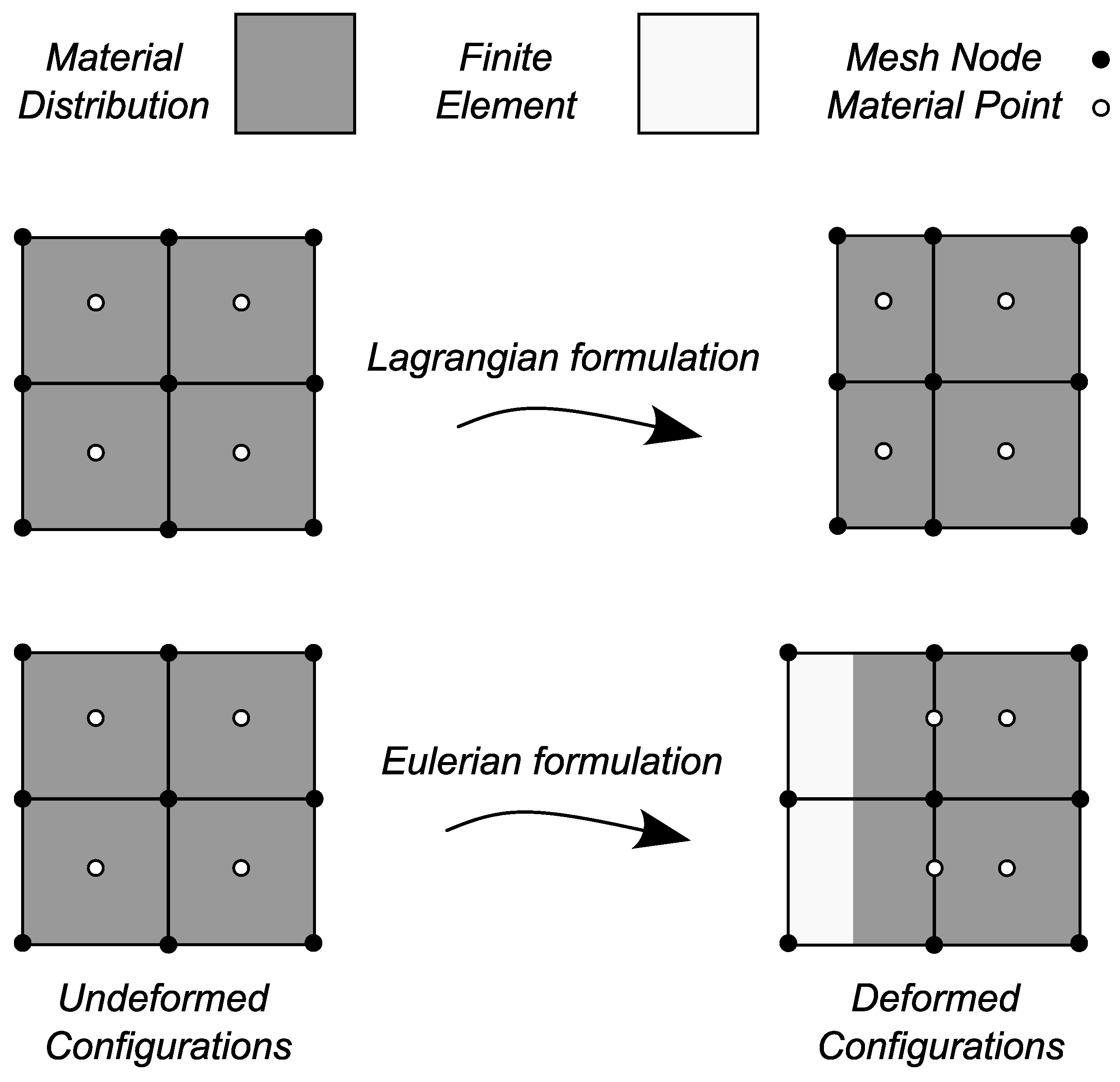
3.2. Arbitrary Lagrangian–Eulerian Method

Based on the virtual work principle, when a virtual displacement field $\delta u$ satisfies the boundary displacement requirements [44], equilibrium is achieved if

$$\begin{array}{c}\hfill {\int }_V\delta {\epsilon }^T\sigma dV+{\int }_V\delta u^T\rho \ddot{u}dV-{\int }_V\delta u^{T}bdV-{\int }_S\delta u^{T}RdS\\ \hfill +{\int }_{{\Gamma }^c}({\sigma }_n\delta g_n+{\sigma }_t\delta g_t)dS=0\end{array}$$

(19)

where $\mathsf{\sigma }$ is the Cauchy stress tensor, $\mathsf{\rho }$ is the density, $\mathsf{\delta }\mathsf{\epsilon }$ indicates the variation of the strain tensor derived from the virtual displacements, $\ddot{\mathit{u}}$ is the acceleration vector, $\mathit{R}$ is the distributed force acting on the boundary $\mathit{S}$ of the volume $\mathit{V}$, $\mathit{b}$ is the body force vector, ${\mathsf{\Gamma }}_{\mathit{c}}$ is the boundary where contact occurs, ${\mathsf{\sigma }}_{\mathit{n}}$ and ${\mathsf{\sigma }}_{\mathit{t}}$ are, respectively, the normal and tangential stresses at the contact surface, and $\mathsf{\delta }{\mathit{g}}_{\mathit{n}}$ and $\mathsf{\delta }{\mathit{g}}_{\mathit{t}}$ are, respectively, the virtual normal and tangential gaps.

Equation (19) is solved incrementally in nonlinear analyses by mapping variables onto a known configuration, either the initial state or the configuration at time t. The Updated Lagrangian (UL) formulation refers to the most recent (i.e., current) equilibrium configuration at each time step, while the Total Lagrangian (TL) formulation uses the reference (i.e., original) configuration at $t=0$. The UL formulation is preferred for situations with large-slip contact.

In the situation of large deformation analysis, using the Lagrangian formulations will inevitably result in severe mesh distortion, reduce the precision of the analysis, or also lead to a negative Jacobian. Separating the material displacements and mesh is one way to prevent mesh distortion. As a result, material points and mesh nodes move in an arbitrary manner [45]. This technique is the core concept of the ALE method. This method integrates the benefits of Eulerian and Lagrangian formulations.

The Eulerian and Lagrangian approaches are the two basic approaches to problems involving the motion of deformable materials [33]. The material points move with the mesh nodes in a Lagrangian description, as shown in Figure 3. Severe mesh deformation can occur because the mesh deforms with the material. The mesh is fixed in space in the Eulerian description, while the material moves through. Because the mesh is fixed, there is no mesh distortion, as presented in Figure 3.

The ALE method proposed in this study is based on the operator-split technique [46]. This approach adds a further Euler step after each UL step [31]. In the UL step, Equation (19) can be solved using the UL method. But it is likely that the mesh will be distorted at the end of the UL step due to the material points being advected along with the mesh nodes. Then comes the Euler step in which a new mesh is created for the distorted mesh, maintaining the original topology while preventing element deformation. After that, all the kinematic and static parameters from the prior mesh are transferred into the current mesh.

4. Validation of the Numerical Model

4.1. Field Experiments

First, the numerical models of jacked piles are validated using data collected from field experiments conducted in Bothkennar, Scotland. These experiments were conducted using the Imperial College instrumented displacement pile (ICP), which was tested in a soft and sensitive marine clay soil [35]. Comprehensive geotechnical investigations were conducted using sampling methodologies, laboratory analyses, and in situ testing procedures to assess the underground conditions. The stratigraphic profile observed at depths ranging from 1 to 6 m revealed a soil composition of soft black silty mottled clay with occasional silt laminae. This primary stratum is overlaid by a weathered firm crust approximately 1 m thick. In situ investigations at the site involved vertical measurements of stress and excess pore pressure using piezometers. Lehane [35] conducted a series of pile installation tests using instrumented steel tubular piles with a diameter of 102 mm, featuring a cone-shaped end with a 60° angle. The piles were pushed into the ground at a constant rate of 10 mm/s, with each push resulting in a 200 mm penetration followed by a pause. They were installed from the bottom of a 1 m deep cased hole to final depths of either 3.2 or 6 m, as illustrated in Figure 4. Three instrument clusters were strategically positioned along the lower 3 m of the pile. These clusters were equipped with various sensors designed to measure the axial load, radial stress, shear stress, and pore pressure, as shown in Figure 4. The specific instrumentation configuration was in accordance with the methodology detailed by Bond [47]. The pile test results were categorized based on their timing during pile installation (jacking), during post-installation as stresses stabilized, and during load testing to failure. In this paper, this validation focuses specifically on the pile jacking phase findings.

4.2. Finite Element Model

The results presented in this study were obtained using the commercial finite element software ABAQUS. Figure 5 illustrates the axisymmetric two-dimensional geometry of the numerical model deployed in pile installation, along with a schematic representation of soil stratification. Figure 5 shows that the water table is located 1 m below the ground surface. The analysis used an axisymmetric soil domain with dimensions of 3 m in radius (approximately 60 times the pile radius) and 8 m in depth, which was considered sufficient for this study. The simulated pile possessed a radius of 0.051 m and an overall length of 6 m. Its tip featured a conical geometry with an apex angle of 60°, which conformed to the specifications of the ICP [47]. The soil nodes on the right were allowed to move vertically, while those at the bottom boundary remained fixed. The axis of symmetry was located on the left boundary, as depicted in Figure 5.

For both the pile and soil domains, the mesh was discretized using four-noded axisymmetric quadrilateral elements. To account for pore pressure effects, four-node axisymmetric elements with pore pressure degrees of freedom (CAX4P) were used for the soil domain. Considering the influence of mesh size on solution convergence and to mitigate computational expense alongside geometric and material nonlinearities, the approach implemented adheres to the methodology used in studies by Sheng [16] for selecting an appropriate mesh size for the soil and pile.

To examine the influence of mesh size on analysis accuracy, three distinct scenarios were developed based on element dimensions. The element size was progressively increased with distance from the axis of symmetry. The ALE method was applied within a localized region extending four radii (4R) from the pile–soil interface to mitigate mesh distortion in the finely discretized domain. The radial thickness of the soil elements beneath the pile tip was defined as follows:

• Fine mesh: Approximately half of the pile shaft radius.
• Medium mesh: Equal to the pile shaft radius.
• Coarse mesh: Two times the pile shaft radius.

If the thickness of the soil elements beneath the pile tip is less than half of the pile shaft radius, numerical instability arises, preventing solution convergence. The considered three scenarios are outlined in

Table 1. Mesh properties.

Mesh	Element Sizes (m)	Total N Elements
Coarse	0.1	425
Medium	0.05	1249
Fine	0.025	3862

and shown in Figure 6.

The Coulomb friction law is employed to model constitutive behavior at the soil–pile interface, using the penalty method for contact treatment. Soil–pile interfaces are discretized using the node-to-segment (NTS) approach. Sheng et al. [2] originally described the NTS approach, which involves master segments on the pile and slave nodes on the soil interface. The primary advantage of NTS discretization is its ability to accommodate both small and large strains, including significant relative sliding at the contact area. In this study, soil properties were derived from the study of Rezania et al. [36]. The dry crust layer, extending from the surface to a depth of 1 m, was modeled using the Mohr–Coulomb material model. The remaining depth of the soil represents the lower layer, which consists of Bothkennar Clay and was represented using the Modified Cam-Clay model. The material properties utilized in the analyses are summarized in

Table 2. Pile and soil properties used in the numerical modeling [36].

Property	Value
Weathered Firm Crust
Elastic modulus (MPa)	3
Poisson’s ratio, $\nu$	0.2
Cohesion (kPa)	6
Friction angle, $\varphi$	30°
Dilation angle, $\psi$	0°
Dry unit weight (kg/m3), ${\gamma }_d$	1900
Bothkennar Clay
$\lambda$	0.3
Poisson’s ratio, $\nu$	0.2
$\kappa$	0.02
M	1.5
Initial void ratio, $e_0$	2
Permeability (m/s), k	$5.96\times {10}^{-5}$
OCR	1.5
Lateral stress coefficient, $K_0$	0.5
Saturated unit weight (kg/m3), ${\gamma }_{sat}$	1650

. The steel pile was represented as a linear elastic material characterized by a volumetric weight of 7750 kg/m³, a Young’s modulus of 210 GPa, and a Poisson’s ratio of 0.3.

In all analyses of this study, the pile is initially located above the ground surface. Two steps are used to model this example.

Firstly, a geostatic analysis was performed where the pile would be primarily situated above the soil surface. Before installing the pile, gravity loading is used to establish the initial in situ stress states in the soil. The lateral stress coefficients and soil unit weights that govern these initial stresses were specified as $K_0$ = 0.5. The pile is then progressively inserted into the clay.

An implicit solver was adopted to simulate the entire pile installation procedure in Bothkennar clay. Small load increments were used in the analysis. Due to the significant nonlinearities arising from frictional contact, large deformation, and elastoplasticity, obtaining convergence to a stable solution presents a major challenge in this type of numerical analysis. To resolve the governing nonlinear system of equations, the Newton iteration procedure was implemented.

4.3. Results and Discussion

In this section, the numerical analysis results are compared with the field experimental data. The graphs illustrate how mesh size affects the solution, as well as the pile-end bearing capacity and radial total stress during installation, along with the experimental measurements. To provide context, the instruments are referenced by their distance from the pile tip $\left(h\right)$ normalized by the pile radius $\left(R\right)$. Graphs of the radial total stress ${\sigma }_r$ measured during installation at $h/R$ ratios of 8 and 28 are included.

4.3.1. Mesh Size Effect

The present study, as shown in Figure 7, investigates the influence of mesh size on pile-end bearing capacity during the installation of the pile. The total stresses in the upper nodes of the pile were assessed. The results show a clear correlation between mesh refinement and the accuracy of the stress predictions. The coarse mesh consistently overestimated the stress values, particularly at greater depths, and exhibited pronounced oscillations that may not accurately reflect the actual pile behavior. The medium mesh offered an intermediate level of accuracy with reduced oscillations compared to the coarse mesh. The fine mesh demonstrated the most reliable stress predictions, as it was characterized by minimal oscillations and a smoother stress distribution.

The oscillations observed in the numerical modeling of pile penetration depend on several factors. Among them, the oscillations are significantly influenced by the size of soil elements used in the mesh discretization—with the amplitude of oscillations proportional to the element size, finer meshes lead to less-pronounced oscillations. The presence of sharp corners or transition points on the geometry of the penetrating pile is a major contributor [2], as soil nodes passing these points experience sudden changes in contact stress directions, causing drops in the vertical reaction force [16]. The NTS approach plays a pivotal role, particularly when applied in conjunction with linear segments representing the pile surface; it is directly associated with the oscillations due to its strong projection of contact constraints. Furthermore, the choice of the penalty parameter can influence oscillations [2], as high penalty values stiffen the contact area and causing smooth oscillations even with a smoothed pile tip.

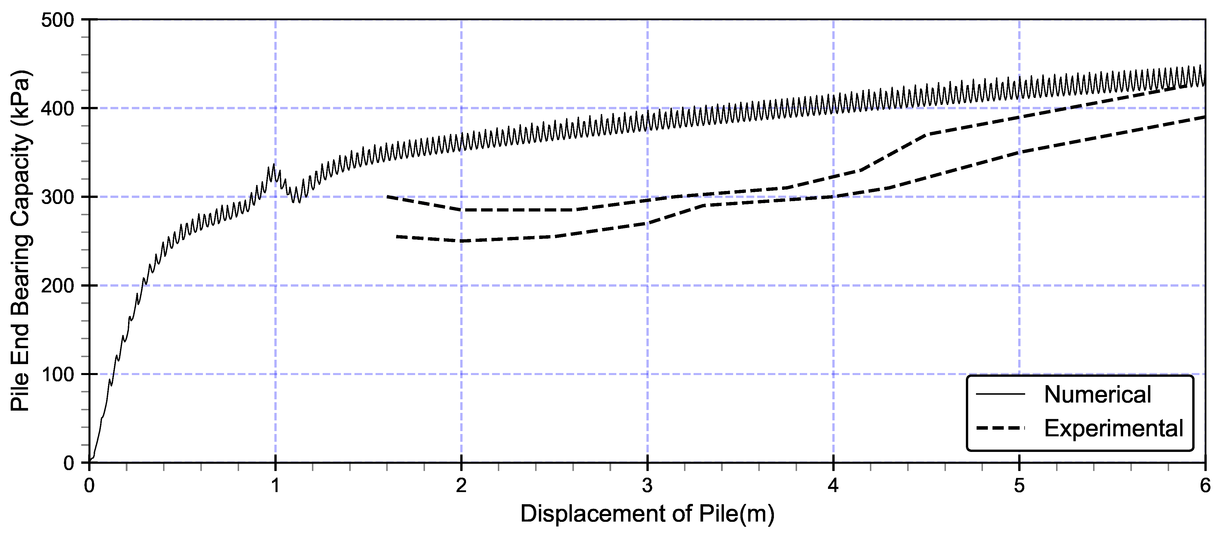
4.3.2. Pile-End Bearing Capacity

Figure 8 presents a comparative analysis of the pile-end bearing capacity between numerical simulations and experimental measurements during jacked pile installation in Bothkennar Clay. The fine mesh was preferred in this analysis, due to its superior reliability in accurately. The numerical results (solid line) closely align with the experimental data (dashed line), demonstrating that the numerical model can capture the stress response at varying depths. However, discrepancies may arise due to differences in installation procedures. The numerical analysis assumes continuous pile installation from 0 to 6 m, whereas the experimental setup involved pre-drilling the uppermost 1 m layer. This variation could influence the stress development near the interface between the weathered crust and the clay stratum, potentially explaining the deviations in the early stages of pile penetration. Nonetheless, the overall agreement suggests the numerical model effectively replicates the end-bearing stress behavior observed in the experiment.

4.3.3. Radial Total Stress During Installation

Figure 9 shows a comparison between experimental tests and numerical analysis results for radial total stress ${\sigma }_{ri}$ during pile installation, where stress values are plotted against displacement. The numerical results (solid lines) and experimental data (dashed lines) are presented at two normalized distances from the pile tip: $h/R$ = 8 (blue lines) and $h/R$ = 28 (red lines).

At $h/R$ = 8, the numerical and experimental stress values align closely, with both peaking at approximately 68 kPa at a displacement of around 1.4 m, followed by a gradual increase to 172 kPa at a displacement of 5.6 m, indicating a strong correlation. At $h/R$ = 28, the numerical results slightly overestimate the stress compared to the experimental data, starting at around 68 kPa and rising to 132 kPa at 5.6 m displacement, whereas the experimental data start from 25 kPa and reach approximately 125 kPa, suggesting a divergence of about 6%. Overall, the numerical model effectively captured the trend of the radial total stress, with a better match at $h/R$ = 8 than at $h/R$ = 28, highlighting the influence of the distance from the pile tip on the radial total stress distribution during installation.

In summary, the modified Cam-Clay model provides a satisfactory approximation of Bothkennar Clay behavior during pile installation. A notable correlation between the predicted and measured values suggests that the proposed model is capable of accurately simulating pile penetration into the soil from the ground surface to the designated depth, when utilizing the implicit time integration scheme.

The discrepancies between the experimental and numerical results can be attributed to various factors. One approach to improving accuracy would be to refine the mesh elements. However, this could lead to distortion and increased computational cost. To address this issue, adaptive mesh refinement was proposed and applied to regions of high interest in explicit and implicit time schemes. Additionally, the application of the ALE method in explicit and implicit time integration has been investigated to mitigate mesh distortion and enhance solution convergence.

5. ALE Method in Explicit and Implicit Time Integration

As shown in the previous section, pile installation in Bothkennar soil layers was successfully executed from the surface to the designated depth, using Modified Cam-Clay (MCC) and Mohr–Coulomb (MC) constitutive models for validation through numerical analysis. While the results exhibited a strong correlation, several limitations were identified, including the impediment that prevented reduction in the soil element thickness beneath the pile tip to less than half of the pile shaft radius—this is due to significant deformations, elastoplastic behavior, and frictional contact at the pile–soil interface. Key challenges included severe distortion of soil elements near the penetrating pile. Moreover, the friction coefficient presented notable constraints for validating the numerical model. To address these computational challenges, the ALE re-meshing method was implemented across explicit and implicit time integration schemes. This approach was selected to mitigate soil element distortion, facilitate the application of appropriate friction coefficients, accurately represent pile–soil interface behavior, and reduce computational demands. The present investigation provides a comparative analysis of the ALE method across explicit and implicit time integration schemes. This study investigates pile behavior under sandy soil conditions by examining various pile dimensions and soil–pile interface friction coefficients, and the effect of dilation angle on pile resistance. The numerical analyses were conducted under dry soil conditions, deliberately excluding pore water pressure considerations from the scope of investigation.

5.1. Numerical Model

The numerical model incorporates the essential pile geometry parameters, soil domain boundaries, and material characteristics. Two different pile diameters, 1 m and 0.5 m, were considered in the model, with the pile length set to 10 times the diameter (10D), where D represents the pile diameter. The soil domain boundaries were established at horizontal and vertical distances of 10D and 20D, respectively, based on research conducted by Dijkstra [48]. Regarding boundary conditions, the bottom boundary was configured with fixed nodes, and vertical displacement was permitted along the right boundary. The left boundary was designated as the axis of symmetry, and the complete geometric configuration and boundary conditions are illustrated in Figure 10.

The constitutive behavior of both the pile and soil domains was represented through the Mohr–Coulomb model, with constituent material properties listed in

Table 3. Pile and soil properties used in the numerical model.

Property	Value
Pile
Elastic modulus (GPa)	25
Poisson’s ratio, $\nu$	0.3
Soil
Elastic modulus (MPa)	10
Poisson’s ratio, $\nu$	0.3
Cohesion (kPa)	1
Friction angle, $\varphi$	37°
Dilation angle, $\psi$	0–8°
Density (kg/m3), $\gamma$	1700

[49]. The analyzed pile comprised a concrete structure with a circular cross-section and a closed-end configuration, whereas the soil medium was represented by Baskarp sand.

The model of pile penetration into sandy soil is axisymmetric. Various types of elements are employed to suit distinct solution schemes. The explicit analysis uses four-node bilinear axisymmetric quadrilateral elements with reduced integration and hourglass control (CAX4R), whereas the implicit analysis implements linear quadrilateral axisymmetric elements with four integration points (CAX4). These elements are applied to both the soil and pile elements. The original finite element mesh is shown in Figure 11.

The numerical analysis was conducted in two stages identical to the validation numerical model. Initially, the soil was subjected to an analysis to determine the initial in situ stress states. Subsequently, the penetration process commenced from the ground surface. In the explicit solver, a constant downward vertical velocity of 250 mm/s was imposed. In contrast, within the implicit solver, the pile is inserted into the soil to a depth of 9D by imposing prescribed displacements at the pile top nodes.

The mesh refinement strategy incorporates soil elements with radial dimensions equivalent to one-fifth of the pile radius in the vicinity of the pile, to optimize computational efficiency. For the ALE method, the remeshing sweep per increment and frequency are both set to five.

The soil–pile interaction is modeled through a master–slave contact formulation, where the pile surface acts as the master surface and the deformable soil medium constitutes the slave surface in a node-to-surface contact approach. For the contact property, the tangent behavior was specified using the penalty method for each of the respective schemes. As for the normal behavior, hard contact was used in the case of an explicit analysis, and the penalty method was added in implicit analysis. The penalty value is defined as ${10}^5$ kN/m³. The soil–pile interface behavior in these models is governed by the penalty method for contact enforcement and the law of Coulomb friction for constitutive response. The interface friction coefficient $\mu$ is parametrically varied between 0 and 0.3 to assess its influence on pile resistance response.

5.2. Results and Discussion

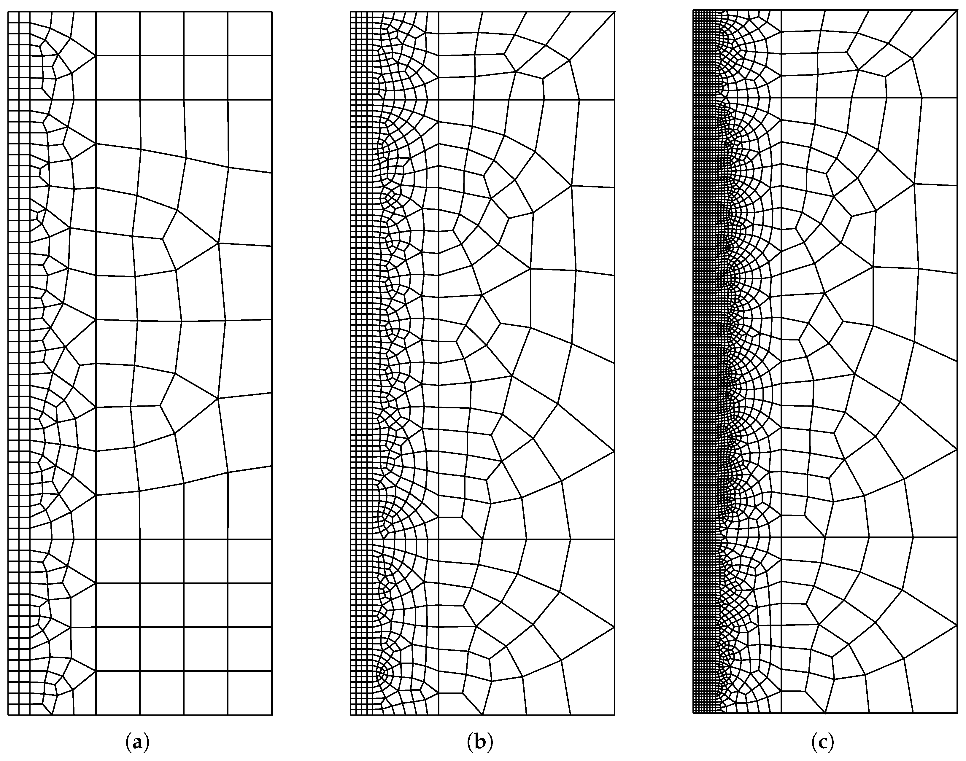
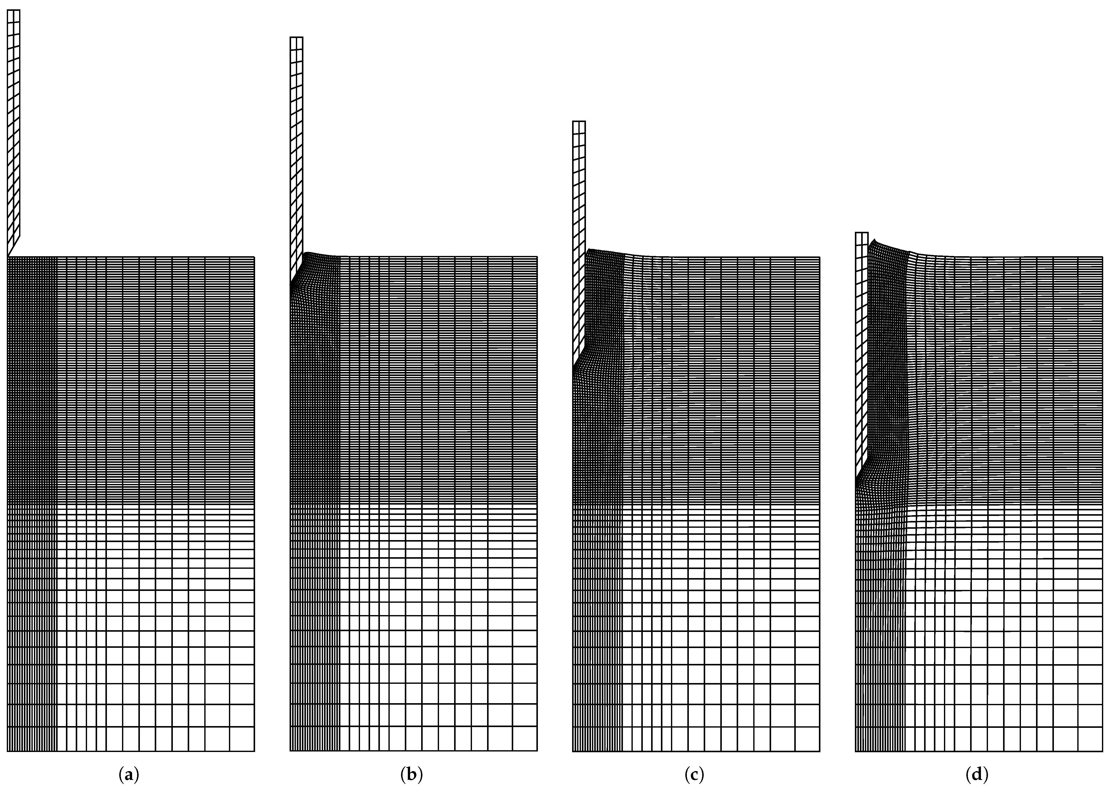
5.2.1. Deformation of the Mesh at Different Depths of Installation

Figure 11 presents the displacement of a pile with a diameter of 0.5 m at different depths, as determined through a simulation using the ALE method. A soil–pile interface friction coefficient of 0.3 was applied. The ALE method is implemented within a soil domain that extends 2D in width from the axis of symmetry and 10D in length. This domain size was selected to optimize computational efficiency while maintaining analysis accuracy. The results indicate that the pile was accurately modeled from the soil surface to the target depth without inducing substantial mesh distortion, highlighting the efficacy of the ALE method in remeshing. Furthermore, Figure 11 illustrates that, as predicted by the Mohr–Coulomb model under shear, the dilatancy behavior leads to a notable increase in soil volume during pile penetration when considering the dilation angle $\psi =8°$, as observed at depth of 9D. The compression of the mesh resulting from pile installation further indicated that substantial radial and vertical deformations were predominantly localized within the initial column of soil elements adjacent to the pile.

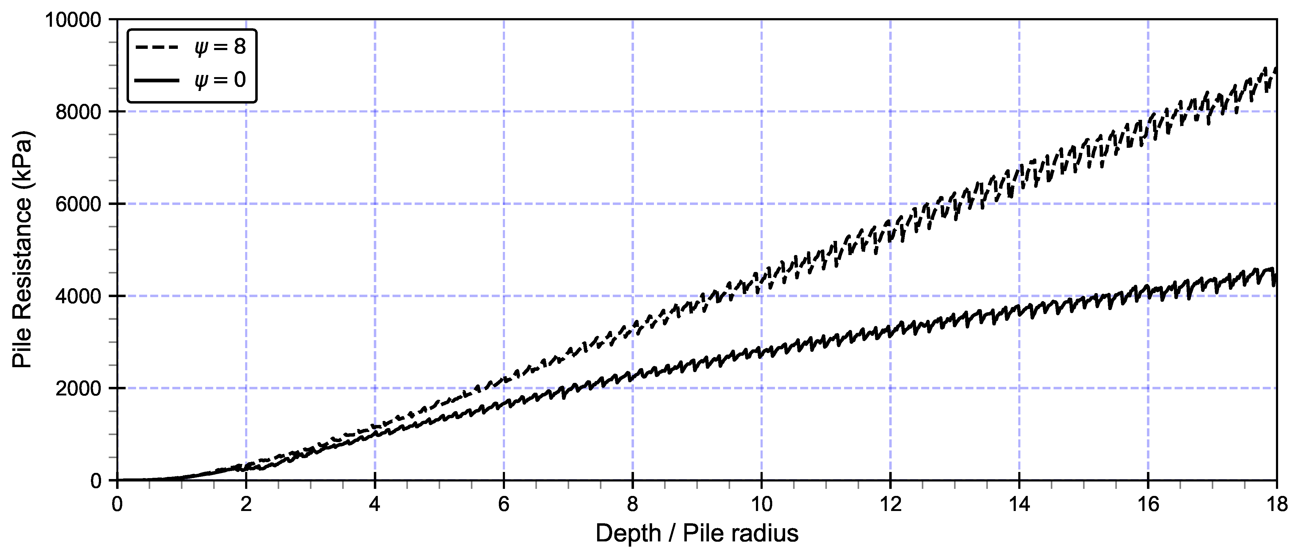
5.2.2. Effect of Dilation Angle on Pile Resistance

Figure 12 illustrates the effect of the dilation angle ($\psi$) on the pile resistance during jacked installation in sand, comparing $\psi =0°$ and $\psi =8°$ with a pile–sand interface friction coefficient of 0.3. The results show that the pile resistance is significantly higher when $\psi =8°$ (dashed line) compared to $\psi =0°$ (solid line). This can be attributed to the fact that higher dilation angles reduce the ability of the sand to expand freely, increasing the confining stress around the pile and enhancing the shaft resistance. In contrast, when $\psi =0°$, the sand dilates more readily under shear, leading to lower confinement and reduced pile resistance. This indicates that dilation plays a crucial role in controlling the skin friction and overall bearing capacity of the pile.

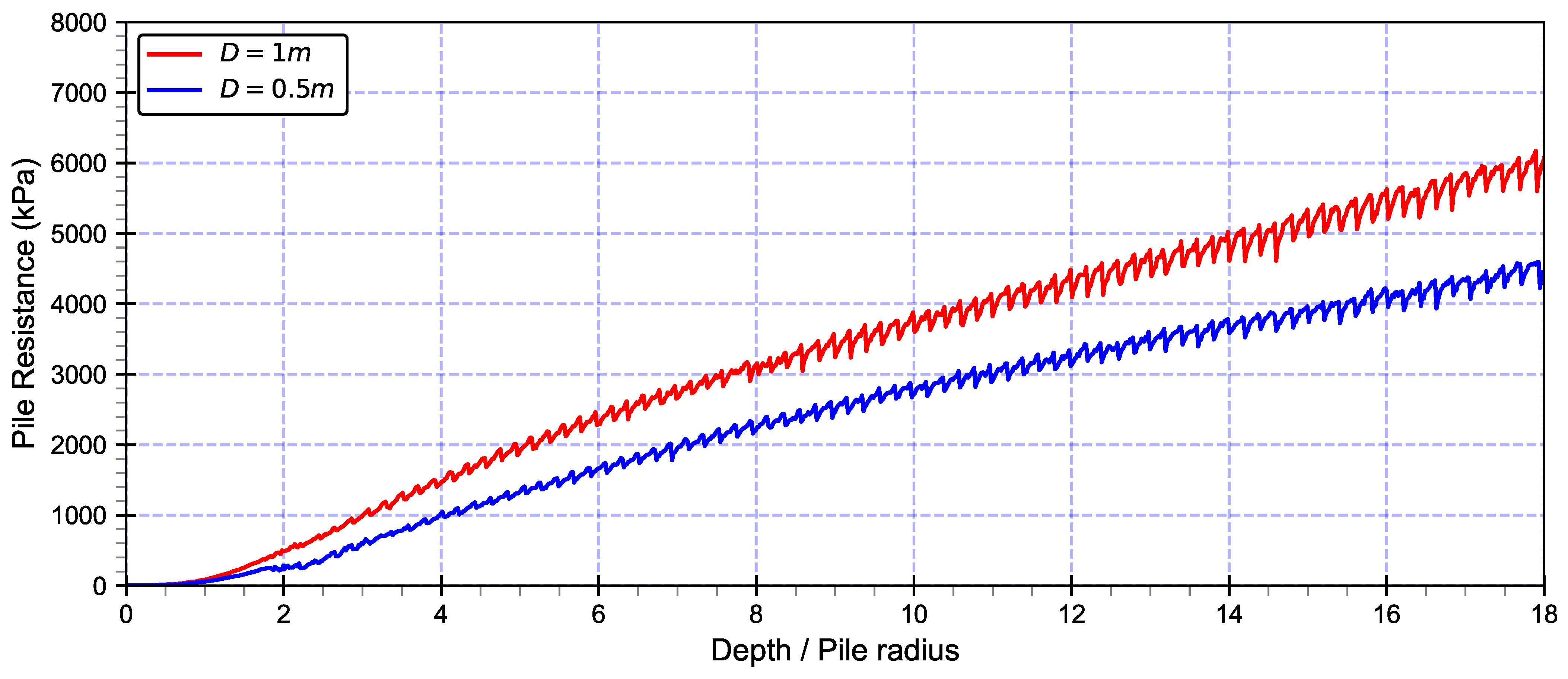
5.2.3. Effect of Pile Dimensions on Pile Resistance

Figure 13 illustrates the total resistance $\left(Q_t\right)$ encountered during pile installation for two different pile diameters, 1.0 m (red line) and 0.5 m (blue line). The total resistance consists of two main components [50], the pile-end resistance $\left(Q_c\right)$ and the shaft friction resistance $\left(Q_s\right)$, which follow the relationship $Q_t=Q_c+Q_s$. The 1.0 m diameter pile consistently showed higher total resistance compared to the 0.5 m pile throughout the installation depth, reaching approximately 6.0 MPa and 4.5 MPa, respectively. Thus, the larger pile is approximately 33% greater than the smaller one.

This significant difference can be explained through both components of the resistance. For the cone resistance $\left(Q_c\right)$, the larger pile has four times the base area $A_L=0.785$ m² compared to the smaller pile, which had the base area $A_S=0.196$ m², which directly increased the pile-end resistance.

For the shaft friction resistance component $\left(Q_s\right)$, a larger length creates twice the shaft surface area along the pile length, combined with a constant friction coefficient of 0.3, which enhances skin friction. The larger pile also displaces more soil during installation, leading to greater soil disturbance and higher lateral Earth pressure against the pile surface, which significantly impacts pile resistance.

5.2.4. Influence of Soil–Pile Interface Friction on Pile Resistance

Figure 14 presents a comparative analysis of explicit and implicit time integration schemes within the ALE method for soil–pile interaction, emphasizing the role of shaft friction resistance in overall pile resistance. The results demonstrate that increasing the friction coefficient ($\mu$) from 0.0 to 0.3 leads to a progressive rise in total pile resistance. Explicit simulations (solid lines) exhibit oscillatory behavior but successfully compute results up to $\mu =0.3$, whereas the implicit scheme (dashed lines) ensures smoother curves but fails at $\mu =0.3$ due to numerical instability. Notably, for $\mu =0.2$, the explicit approach predicts a resistance approximately 35% higher than the $\mu =0.0$ case, while the implicit counterpart estimates around a 30% increase.

The oscillations observed in Figure 14 are more pronounced in explicit analyses than in implicit analyses, where such oscillations are notably subdued. The ALE method helps reduce mesh distortion and allows for finer meshes, which lessens these oscillations, but they can still be noticed. A primary factor in these oscillations, beyond the influence of mesh element size, is the presence of sharp corners or vertices on the master surface, such as the transition between the tip and the shaft of a pile. Implementing a smooth discretization of the master surface in the contact algorithm employed in implicit analyses substantially diminishes the oscillations in pile resistance compared to the use of linear segments. However, such smooth discretization is not feasible in the contact algorithm of explicit analyses, which relies on a kinematic contact method. Furthermore, oscillations arise in explicit analyses from high-frequency modes that are inadequately damped, owing to the absence of inherent numerical damping.

Based on these meticulous observations, one can conclusively determine that the ALE method exhibits superior performance when coupled with explicit time integration schemes, particularly in terms of numerical stability and mitigating potential computational issues. Although the implicit scheme provides ostensibly smoother solutions, its pronounced limitation at higher friction coefficients strongly suggests that the explicit scheme may represent a more robust approach for modeling frictional soil–pile interactions using the ALE method, notwithstanding its characteristic oscillatory behavior. This result highlights the critical influence of shaft friction resistance on pile behavior.

Interface soil–pile behavior according to Coulomb’s law for frictional contact problems is manifested in three distinct states—contact with adherence, contact with slip, and non-contact—as described in Section 2.

Figure 15 illustrates the variation of normal and tangential contact stresses as a function of pile displacement for both explicit and implicit time integration schemes, considering a friction coefficient of 0.2 and a pile with a diameter of 0.5 m.

In implicit time integration, within the range of 0 to 0.2 m, non-contact is observed between the soil and the pile, as indicated by ${\sigma }_n=0$. Beyond 0.2 m, up to the completion of pile installation, contact is established between the soil and pile, with ${\sigma }_n>0$. Within this interval, both the normal and tangential contact stresses reach their maximum values at a depth of 3.9 m, where ${\sigma }_n=250$ kPa and ${\sigma }_t=-50$ kPa. Given that $|{\sigma }_t|=\mu {\sigma }_n$, contact with slip occurs within this range, thus satisfying the Coulomb friction law.

Similarly, when using explicit time integration, non-contact is observed between the soil and the pile from 0 to 0.2 m, as ${\sigma }_n=0$. For depths exceeding 0.2 m until the end of pile installation, contact is established with ${\sigma }_n>0$, as seen in Figure 15. The maximum values of the normal and tangential contact stresses were recorded at a depth of 4.15 m, where ${\sigma }_n=206$ kPa and ${\sigma }_t=-41$ kPa. Because $|{\sigma }_t|=\mu {\sigma }_n$, contact with slip is present within this interval, which conforms to the Coulomb friction law.

Although the two methods exhibit a slight difference due to their use of a different contact property, both effectively capture the interface behavior between the soil and pile. The validation of Coulomb’s friction law verifies the accurate representation of the soil–pile interface behavior in the numerical model of pile installation.

5.2.5. Computational Efficiency

The computational performance analysis of pile penetration simulation using the ALE adaptive mesh method revealed significant distinctions between explicit and implicit time integration schemes shown in

Table 4. Computational efficiency in explicit and implicit schemes.

Schemes	CPU Time (s)	Increments
Explicit	370	106,051
Implicit	1569	10,014

. The numerical simulations were conducted with a friction coefficient of 0.1, conducted on a Lenovo laptop equipped with an AMD Ryzen 5500 processor operating at 2.1 GHz and 8 GB RAM. The explicit time integration scheme completed the analysis in 370 s, requiring 106,051 increments, whereas the implicit scheme required 1569 s with 10,014 increments to solve the problem. This disparity arises from fundamental differences in their formulations. Explicit schemes, leveraging diagonalized mass matrices and avoiding iterative solutions, achieves low computational cost per increment despite necessitating small time steps for stability in the installation of pile. Conversely, implicit schemes, while permitting larger steps due to unconditional stability, demand costly matrix inversions and iterative solutions per increment, significantly increasing the time per step. For this simulation, explicit efficiency dominates because the problem inherently requires small increments to resolve frictional contact and large deformation nonlinearities, underscoring the suitability of the explicit method for nonlinear problems with ALE adaptive meshing.

6. Conclusions

In this research, the ALE method was effectively applied to model the complete penetration of a pile from the ground surface. The simulation included the frictional contact between the soil and pile. The numerical pile penetration model was initially validated against field experiments conducted for Bothkennar clay using the ICP.

The MCC model adequately captured the behavior of Bothkennar clay during pile installation, with good agreement between the measured and calculated values. This validation confirmed the model’s capability to simulate pile penetration from surface to target depth using implicit time integration techniques. Some discrepancies between the experimental and numerical results were observed, which were addressed through mesh refinement strategies.

A comparative analysis of the ALE method implementation in explicit and implicit time integration schemes revealed several key findings:

• The ALE method effectively addressed mesh distortion challenges in both the explicit and implicit schemes without significant computational overhead.
• The computational results from both explicit and implicit schemes indicate that higher interface friction coefficients consistently yield greater total resistance values. Furthermore, the findings indicate that an increase in pile dimension is associated with an enhancement in its overall resistance, primarily due to optimization of the pile-end and shaft friction resistances.
• The explicit time integration scheme demonstrated superior stability and robustness, particularly in cases involving higher friction coefficients, despite characteristic oscillations in the solutions. While the implicit scheme produced smoother solutions, it showed limitations at higher friction coefficients, suggesting reduced effectiveness under complex soil–pile interaction conditions.
• A higher dilation angle ($\psi =8°$) enhances pile resistance by increasing the confining and shaft stress, whereas a lower dilation angle ($\psi =0°$) leads to reduced confinement and lower resistance. These findings align with fundamental principles of soil mechanics, where dilation contributes to increased shear strength and resistance due to volumetric constraints, thereby enhancing the pile resistance.
• The explicit method exhibited lower CPU time requirements, compared to the implicit approach.

These findings establish the ALE method as a viable approach for simulating pile penetration problems, with the explicit time integration scheme emerging as a more robust choice for challenging soil–pile interaction scenarios.

References

1. Sheng, D.; Eigenbrod, K.D.; Wriggers, P. Finite element analysis of pile installation using large-slip frictional contact. Comput. Geotech. 2005, 32, 17–26. [Google Scholar] [CrossRef]
2. Fischer, K.A.; Sheng, D.; Abbo, A.J. Modeling of pile installation using contact mechanics and quadratic elements. Comput. Geotech. 2007, 34, 449–461. [Google Scholar] [CrossRef]
3. Zhang, M.; Sang, S.; Wang, Y.; Bai, X. Factors Influencing the Mechanical Characteristics of a Pile–Soil Interface in Clay Soil. Front. Earth Sci. 2020, 7, 364. [Google Scholar] [CrossRef]
4. Yoo, B.S.; Tran, N.X.; Kim, S.R. Numerical Simulation of Piles in a Liquefied Slope Using a Modified Soil–Pile Interface Model. Appl. Sci. 2023, 13, 6626. [Google Scholar] [CrossRef]
5. Lehane, B.M.; Jardine, R.; Bond, A.J.; Frank, R. Mechanisms of shaft friction in sand from instrumented pile tests. J. Geotech. Eng. 1993, 119, 19–35. [Google Scholar] [CrossRef]
6. Chow, F.; Jardine, R.J. Investigations into the behaviour of displacement piles for offshore foundations. Ground Eng. 1996, 29, 24–25. [Google Scholar] [CrossRef]
7. Jardine, R.J.; Standing, J.R.; Chow, F.C. Some observations of the effects of time on the capacity of piles driven in sand. Géotechnique 2006, 56, 227–244. [Google Scholar] [CrossRef]
8. Tsuha, C.; Foray, P.; Jardine, R.; Yang, Z.; Silva, M.; Rimoy, S. Behaviour of displacement piles in sand under cyclic axial loading. Soils Found. 2012, 52, 393–410. [Google Scholar] [CrossRef]
9. Arshad, M.I. Experimental Study of the Displacements Caused by Cone Penetration in Sand. Ph.D. Thesis, Purdue University, West Lafayette, IN, USA, 2014. [Google Scholar]
10. Jardine, R.; Zhu, B.; Foray, P.; Yang, Z. Interpretation of stress measurements made around closed-ended displacement piles in sand. Géotechnique 2013, 63, 613–627. [Google Scholar] [CrossRef]
11. Jardine, R.; Zhu, B.; Foray, P.; Yang, Z. Measurement of stresses around closed-ended displacement piles in sand. Géotechnique 2013, 63, 1–17. [Google Scholar] [CrossRef]
12. Rimoy, S.; Silva, M.; Jardine, R.; Yang, Z.X.; Zhu, B.; Tsuha, C.d.H. Field and model investigations into the influence of age on axial capacity of displacement piles in silica sands. Géotechnique 2015, 65, 576–589. [Google Scholar] [CrossRef]
13. Tehrani, F.S.; Arshad, M.I.; Prezzi, M.; Salgado, R. Physical modeling of cone penetration in layered sand. J. Geotech. Geoenviron. Eng. 2018, 144, 04017101. [Google Scholar] [CrossRef]
14. Tovar-Valencia, R.D.; Galvis-Castro, A.; Salgado, R.; Prezzi, M. Effect of surface roughness on the shaft resistance of displacement model piles in sand. J. Geotech. Geoenviron. Eng. 2018, 144, 04017120. [Google Scholar] [CrossRef]
15. Tovar-Valencia, R.D.; Galvis-Castro, A.; Salgado, R.; Prezzi, M.; Fridman, D. Experimental measurement of particle crushing around model piles jacked in a calibration chamber. Acta Geotech. 2023, 18, 1331–1351. [Google Scholar] [CrossRef]
16. Sheng, D.; Nazem, M.; Carter, J.P. Some computational aspects for solving deep penetration problems in geomechanics. Comput. Mech. 2009, 44, 549–561. [Google Scholar] [CrossRef]
17. Qiu, G.; Henke, S.; Grabe, J. Application of a Coupled Eulerian–Lagrangian approach on geomechanical problems involving large deformations. Comput. Geotech. 2011, 38, 30–39. [Google Scholar] [CrossRef]
18. Hamann, T.; Qiu, G.; Grabe, J. Application of a Coupled Eulerian–Lagrangian approach on pile installation problems under partially drained conditions. Comput. Geotech. 2015, 63, 279–290. [Google Scholar] [CrossRef]
19. Fan, S.; Bienen, B.; Randolph, M.F. Effects of monopile installation on subsequent lateral response in sand. I: Pile installation. J. Geotech. Geoenviron. Eng. 2021, 147, 04021021. [Google Scholar] [CrossRef]
20. Bienen, B.; Fan, S.; Schröder, M.; Randolph, M.F. Effect of the installation process on monopile lateral response. Proc. Inst. Civ. Eng.-Geotech. Eng. 2021, 174, 530–548. [Google Scholar] [CrossRef]
21. Staubach, P.; Machaček, J.; Bienen, B.; Wichtmann, T. Long-term response of piles to cyclic lateral loading following vibratory and impact driving in water-saturated sand. J. Geotech. Geoenviron. Eng. 2022, 148, 04022097. [Google Scholar] [CrossRef]
22. Staubach, P.; Machaček, J.; Skowronek, J.; Wichtmann, T. Vibratory pile driving in water-saturated sand: Back-analysis of model tests using a hydro-mechanically coupled CEL method. Soils Found. 2021, 61, 144–159. [Google Scholar] [CrossRef]
23. Liyanapathirana, D. Arbitrary Lagrangian Eulerian based finite element analysis of cone penetration in soft clay. Comput. Geotech. 2009, 36, 851–860. [Google Scholar] [CrossRef]
24. Tolooiyan, A.; Gavin, K. Modelling the cone penetration test in sand using cavity expansion and arbitrary Lagrangian Eulerian finite element methods. Comput. Geotech. 2011, 38, 482–490. [Google Scholar] [CrossRef]
25. Yang, Z.; Gao, Y.; Jardine, R.; Guo, W.; Wang, D. Large deformation finite-element simulation of displacement-pile installation experiments in sand. J. Geotech. Geoenviron. Eng. 2020, 146, 04020044. [Google Scholar] [CrossRef]
26. Spyridis, M.; Lopez-Querol, S. Numerical investigation of displacement pile installation in silica sand. Comput. Geotech. 2023, 161, 105591. [Google Scholar] [CrossRef]
27. Phuong, N.; Van Tol, A.; Elkadi, A.; Rohe, A. Modelling of pile installation using the material point method (MPM). Numer. Methods Geotech. Eng. 2014, 271, 271–276. [Google Scholar] [CrossRef]
28. Fu, S.; Yang, Z.; Guo, N.; Jardine, R. Material point method simulations of displacement pile and CPT penetration in sand considering the effects of grain breakage. Comput. Geotech. 2024, 166, 105945. [Google Scholar] [CrossRef]
29. Hu, Y.; Randolph, M. A practical numerical approach for large deformation problems in soil. Int. J. Numer. Anal. Methods Geomech. 1998, 22, 327–350. [Google Scholar] [CrossRef]
30. Hirt, C.W.; Amsden, A.A.; Cook, J. An arbitrary Lagrangian-Eulerian computing method for all flow speeds. J. Comput. Phys. 1974, 14, 227–253. [Google Scholar] [CrossRef]
31. Nazem, M.; Sheng, D.; Carter, J.P. Stress integration and mesh refinement for large deformation in geomechanics. Int. J. Numer. Methods Eng. 2006, 65, 1002–1027. [Google Scholar] [CrossRef]
32. Susila, E.; Hryciw, R.D. Large displacement FEM modelling of the cone penetration test (CPT) in normally consolidated sand. Int. J. Numer. Anal. Methods Geomech. 2003, 27, 585–602. [Google Scholar] [CrossRef]
33. Belytschko, T.; Liu, W.K.; Moran, B.; Elkhodary, K. Nonlinear Finite Elements for Continua and Structures; John Wiley & Sons: West Sussex, UK, 2014; pp. 329–415. [Google Scholar]
34. Terfaya, N.; Berga, A.; Raous, M.; Abou-Bekr, N. A contact model coupling friction and adhesion: Application to pile/soil interface. Int. Rev. Civ. Eng. 2018, 9, 20. [Google Scholar] [CrossRef]
35. Lehane, B.M.; Jardine, R. Displacement-pile behaviour in a soft marine clay. Can. Geotech. J. 1994, 31, 181–191. [Google Scholar] [CrossRef]
36. Rezania, M.; Mousavi Nezhad, M.; Zanganeh, H.; Castro, J.; Sivasithamparam, N. Modeling pile setup in natural clay deposit considering soil anisotropy, structure, and creep effects: Case study. Int. J. Geomech. 2017, 17, 04016075. [Google Scholar] [CrossRef]
37. Tan, J.P.S.; Goh, S.H.; Tan, S.A. Numerical analysis of a jacked-in pile installation in clay. Int. J. Geomech. 2023, 23, 04023061. [Google Scholar] [CrossRef]
38. Li, L.; Zhou, P.; Li, J.; Huang, L.; Shao, W. Numerical simulation of time-dependent performance of jacked piles in marine clays: Considering anisotropy and destructuration. Ocean Eng. 2025, 322, 120461. [Google Scholar] [CrossRef]
39. Mabsout, M.E.; Tassoulas, J.L. A finite element model for the simulation of pile driving. Int. J. Numer. Methods Eng. 1994, 37, 257–278. [Google Scholar] [CrossRef]
40. Reddy, J.N. Kinematics of a Continuum; Cambridge University Press: Cambridge, UK, 2010; pp. 55–92. [Google Scholar] [CrossRef]
41. Wriggers, P. Computational Contact Mechanics; Springer: Berlin/Heidelberg, Germany; New York, NY, USA, 2006; pp. 11–25. [Google Scholar] [CrossRef]
42. Wriggers, P. Nonlinear Finite Element Methods; Springer: Berlin/Heidelberg, Germany, 2008; pp. 205–215. [Google Scholar] [CrossRef]
43. Newmark, N.M. A method of computation for structural dynamics. J. Eng. Mech. Div. 1959, 85, 67–94. [Google Scholar] [CrossRef]
44. Sheng, D.; Wriggers, P.; Sloan, S.W. Application of Frictional Contact in Geotechnical Engineering. Int. J. Geomech. 2007, 7, 176–185. [Google Scholar] [CrossRef]
45. Donea, J.; Giuliani, S.; Halleux, J.P. An arbitrary Lagrangian-Eulerian finite element method for transient dynamic fluid-structure interactions. Comput. Methods Appl. Mech. Eng. 1982, 33, 689–723. [Google Scholar] [CrossRef]
46. Benson, D.J. An efficient, accurate, simple ALE method for nonlinear finite element programs. Comput. Methods Appl. Mech. Eng. 1989, 72, 305–350. [Google Scholar] [CrossRef]
47. Bond, A.; Jardine, R. Effects of installing displacement piles in a high OCR clay. Geotechnique 1991, 41, 341–363. [Google Scholar] [CrossRef]
48. Dijkstra, J.; Broere, W.; van Tol, A.F. Eulerian Simulation of the Installation Process of a Displacement Pile. In Proceedings of the Contemporary Topics in In Situ Testing, Analysis, and Reliability of Foundations, Orlando, FL, USA, 15 March 2009; American Society of Civil Engineers: Reston, VA, USA, 2009; pp. 135–142. [Google Scholar] [CrossRef]
49. Dijkstra, J.; Broere, W.; van Tol, A. Numerical simulation of the installation of a displacement pile in sand. In Proceedings of the 10th International Symposium on Numerical Models in Geomechanics (NUMOG X), Rhodes, Greece, 25–27 April 2007; pp. 461–466. [Google Scholar] [CrossRef]
50. Frank, R.; Cuira, F.; Burlon, S. Design of Shallow and Deep Foundations; CRC Press: New York, NY, USA, 2021; pp. 81–181. [Google Scholar] [CrossRef]
Figure 1. Configurations of two bodies come into contact.
Mca 30 00058 g001
Figure 2. Laws of contact and friction. (a) Normal conditions. (b) Contact with friction.
Mca 30 00058 g002
Figure 3. Undeformed and deformed configurations of the body in Lagrangian and Eulerian formulations.
Mca 30 00058 g003
Figure 4. Pile configurations [35].
Mca 30 00058 g004
Figure 5. Geometry and boundary conditions of the axisymmetric validation model.
Mca 30 00058 g005
Figure 6. Meshes with different sizes. (a) Coarse. (b) Medium. (c) Fine.
Mca 30 00058 g006
Figure 7. Influence of mesh sizes on accuracy of solution.
Mca 30 00058 g007
Figure 8. Numerical analysis and experimental data for pile-end bearing stress at varying depth.
Mca 30 00058 g008
Figure 9. Comparison between field experiment data and numerical analysis results for radial total stress during installation.
Mca 30 00058 g009
Figure 10. Geometry of the axisymmetric model.
Mca 30 00058 g010
Figure 11. Original and deformed meshes at varying penetration depths. (a) Original. (b) At 2.25D. (c) At 4.5D. (d) At 9D.
Mca 30 00058 g011
Figure 12. Effect of dilation angle ( ψ = 0 ° and ψ = 8 ° ) on pile resistance with pile–sand interface friction coefficient of 0.3.
Mca 30 00058 g012
Figure 13. Effect of pile dimensions on results.
Mca 30 00058 g013
Figure 14. Influence of friction coefficient on pile resistance.
Mca 30 00058 g014
Figure 15. Influence of friction coefficient on soil–pile interface. (a) Implicit time integration. (b) Explicit time integration.
Mca 30 00058 g015