Hybrid Neural Network Approach with Physical Constraints for Predicting the Potential Occupancy Set of Surrounding Vehicles

Abstract

The reliable and uncertainty-aware prediction of surrounding vehicles remains a key challenge in autonomous driving. However, existing methods often struggle to quantify and incorporate uncertainty effectively. To address these challenges, we propose a hybrid architecture that combines a data-driven neural trajectory predictor with physically grounded constraints to forecast future vehicle occupancy. Specifically, the physical constraints are derived from vehicle kinematic principles and embedded into the network as additional loss terms during training. This integration ensures that predicted trajectories conform to feasible and physically realistic motion boundaries. Furthermore, a mixture density network (MDN) is employed to estimate predictive uncertainty, transforming deterministic trajectory predictions into spatial probability distributions. This enables a probabilistic occupancy representation, offering a richer and more informative description of the potential future positions of surrounding vehicles. The proposed model is trained and evaluated on the Aerial Dataset for China’s Congested Highways and Expressways (AD4CHE), which contains representative driving scenarios in China. Experimental results demonstrate that the model achieves strong fitting performance while maintaining high physical plausibility in its predictions.

1. Introduction

With autonomous driving technology steadily advancing toward widespread commercial adoption, it has become crucial to ensure its safety for achieving major industry milestones. Accurately forecasting the movements of nearby vehicles is essential for improving the safety of autonomous vehicles [1]. This capability not only aids in effectively evaluating driving risks but also directly influences the safety of autonomous driving systems during planning and decision-making processes.

Vehicle motion prediction methods can generally be classified into two categories: rule-based approaches and data-driven methods. Rule-based models rely on vehicle dynamics or kinematics to estimate future trajectories. Representative techniques include the single-track model [2], Kalman filters [3], and Monte Carlo methods [4]. Althoff et al. [5] extended these models by incorporating physical constraints to estimate reachable sets. These approaches are computationally efficient and interpretable but are typically limited to short-term predictions due to the continuously changing states of traffic participants [6].

Traditional machine learning methods such as support vector machines [7], hidden Markov models [8], and dynamic Bayesian networks [9] introduced early attempts at learning motion patterns from data. However, these approaches often rely on maneuver classification and offer limited flexibility in complex, dynamic traffic environments. Deep learning-based methods have recently gained prominence for their superior fitting ability and long-term forecasting performance. LSTM networks, as an improved variant of RNNs, are widely adopted to capture temporal dependencies and mitigate issues such as vanishing gradients. For example, Altché et al. [10] applied a single-layer LSTM for highway trajectory prediction. Ding et al. [11] proposed an LSTM encoder for maneuver prediction, followed by trajectory estimation using map data. To model multimodal behaviors, Zyner et al. [12] introduced a GMM layer on top of a three-layer LSTM, while Kawasaki et al. [13] integrated LSTM with Kalman filtering for lane-aware prediction. Zhang et al. [14] employed a dual-LSTM architecture for intention and motion prediction. To improve the ability of the model to capture data features, attention mechanisms are frequently integrated into prediction tasks. In [15,16], a multi-head attention mechanism was employed to extract lane and vehicle attention, thereby generating a distribution of future trajectories. In addition to sequence-based models, spatial perception-driven approaches using bird’s eye view (BEV) representations have shown strong performance in structured environments. These models encode lane geometry, map features, and surrounding agents in rasterized form to facilitate spatial reasoning, as demonstrated in works such as [17]. Transformer-based architectures have gained attention for their global attention capabilities and scalability. By replacing recurrent mechanisms with self-attention, these models capture longer-range dependencies more effectively. Notable examples include models that use attention to model agent–agent and agent–map interactions simultaneously [18,19,20]. However, Transformer-based models typically require large-scale annotated data for effective generalization and can suffer from high computational costs during inference, which limits their applicability in real-time or resource-constrained autonomous driving systems.

Despite these advancements, most existing approaches still rely on single-point trajectory prediction, which limits their ability to represent inherent uncertainty. This simplification fails to capture the full range of possible future movements, thereby reducing reliability in real-world applications. Furthermore, recent studies have underscored the importance of generalization and robustness under domain shifts and complex conditions. Banitalebi-Dehkordi et al. [21] proposed a curriculum-based domain adaptation strategy for robust object detection, while Khosravian et al. [22] introduced a multi-domain driving dataset to improve cross-domain generalization. While these works primarily focus on perception tasks, our study complements this research direction by addressing uncertainty-aware, physically grounded trajectory prediction in structured traffic environments.

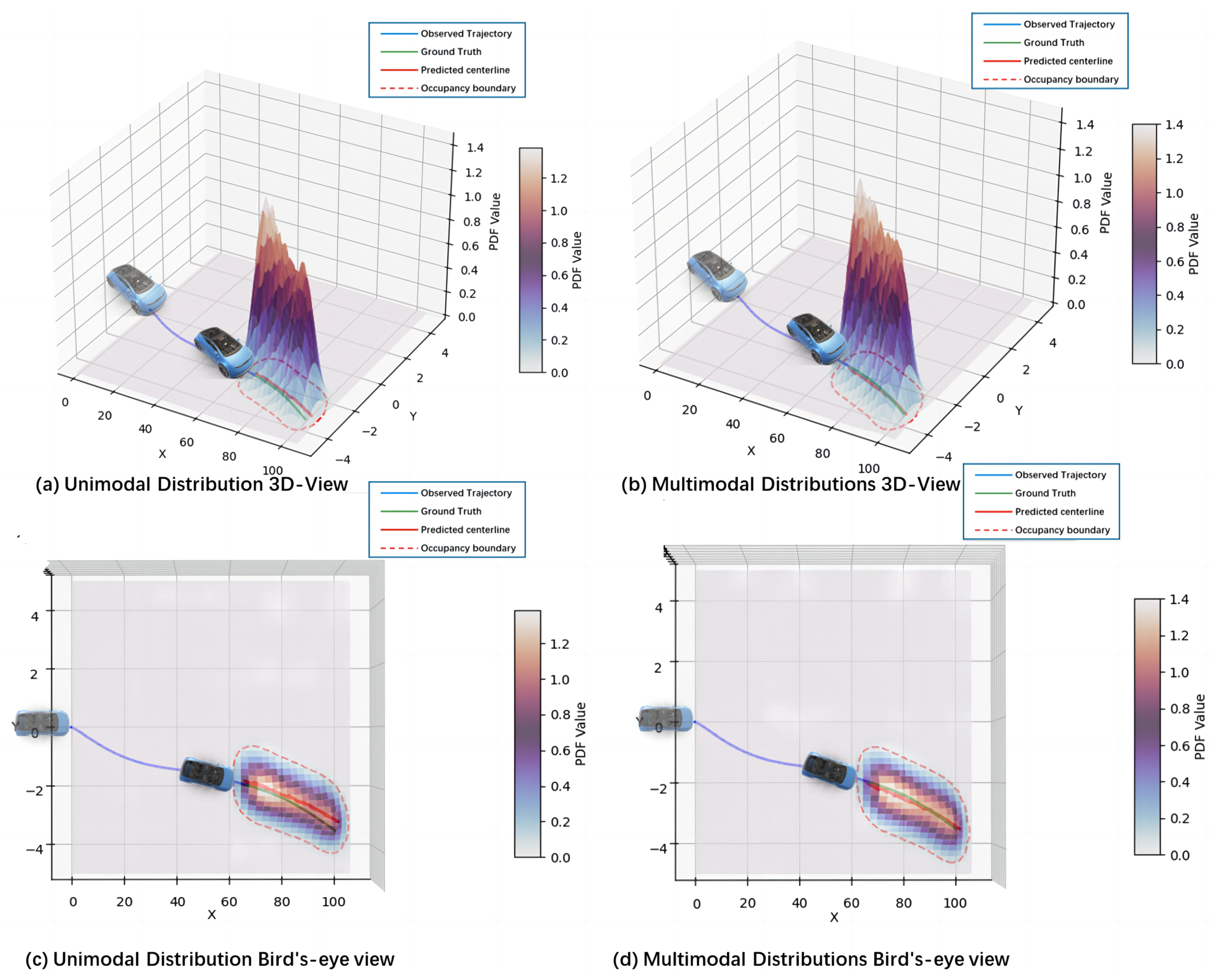
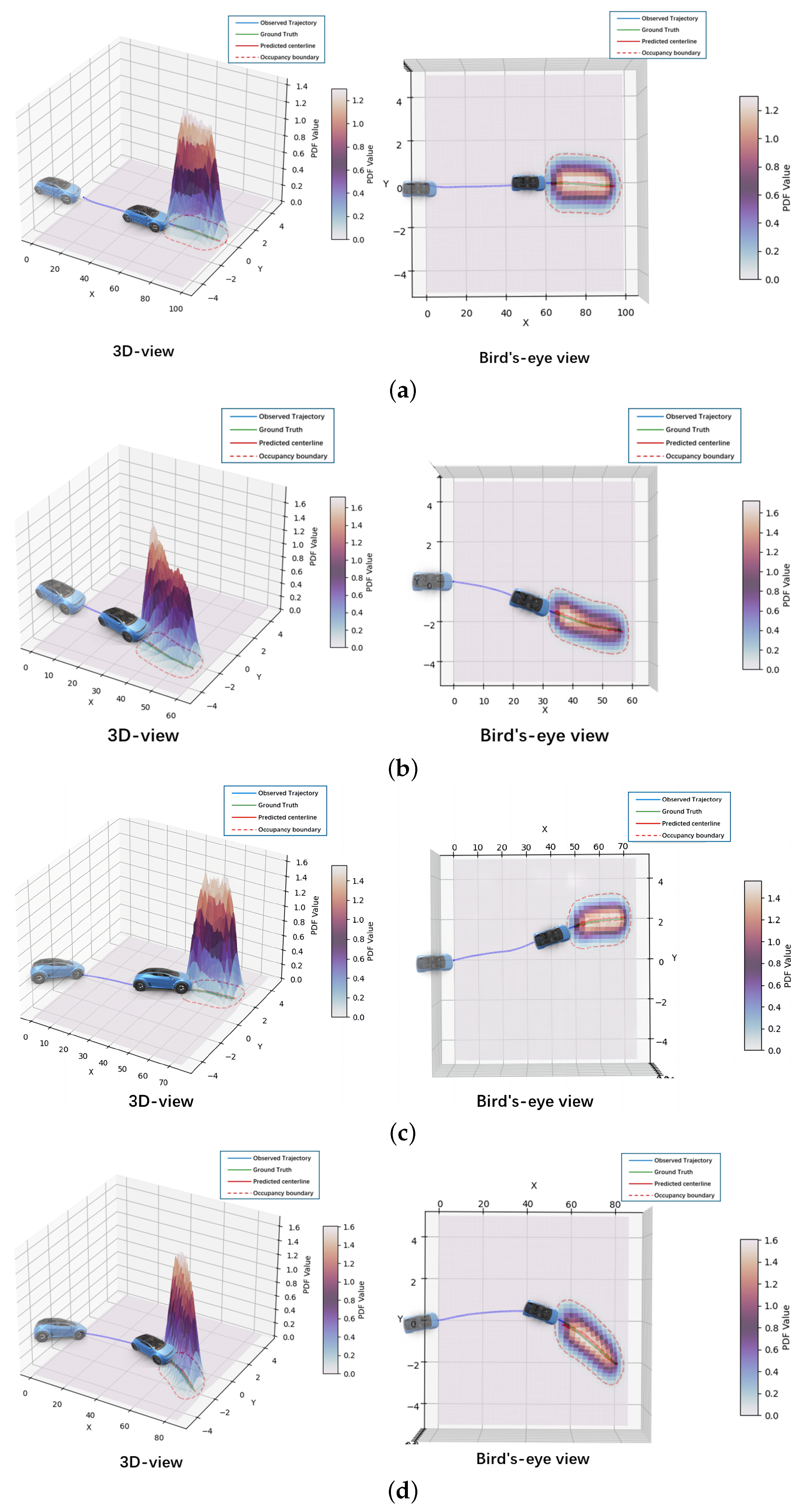
In this study, we propose a hybrid prediction framework that integrates a neural network-based trajectory predictor with physically grounded constraints. The neural component captures complex, data-driven motion patterns, while the physical constraints—derived from vehicle kinematics—are incorporated as additional loss terms to guide the network toward producing feasible and realistic trajectories. The uncertainty of the prediction results was quantified using the mixture density network (MDN) layer in the network. This expands the prediction results from a single-point trajectory to a regional distribution, thereby enhancing the accuracy of future occupancy predictions of surrounding vehicles. The possible movement range of the surrounding vehicles can be more comprehensively reflected by quantifying the prediction uncertainty and generating regional distributions, thereby providing more detailed information. This approach improves the practical reliability of prediction models and provides a more dependable foundation for trajectory planning and safety evaluation in autonomous vehicles. During training, the Aerial Dataset for China’s Congested Highways and Expressways (AD4CHE), which includes typical driving scenarios in China, was used, making the output predictions of the network more aligned with the Chinese traffic environment.

The key contributions of this study can be summarized as follows:

(1)

Adaptation to Chinese Road Scenarios: This study leverages the AD4CHE dataset, which captures typical highway and expressway behaviors in China. Unlike prior work that primarily uses datasets like NGSIM, our approach addresses region-specific driving patterns, offering more practical relevance for autonomous driving in Chinese contexts.

(2)

Feature-Level Attention without Interaction Modeling: Instead of explicitly modeling inter-vehicle interactions, we integrate a squeeze-and-excitation (SE) block into the temporal feature extractor to adaptively highlight informative motion features, enhancing temporal correlation learning.

(3)

Physically Constrained Trajectory Predictions: Physical motion constraints are incorporated to ensure trajectory feasibility, improving the realism and reliability of predictions for downstream planning.

(4)

Uncertainty-Aware Output via Occupancy Sets: The model outputs a multimodal Gaussian mixture distribution, which is projected onto a spatial occupancy set. This allows probabilistic reasoning and better accounts for trajectory uncertainty in real-world scenarios.

The remainder of this paper is structured as follows: Section 2 defines the problem of occupancy set prediction and dataset feature used for training. In Section 3, we outline the network model structure. Section 4 discusses the training process and presents the findings of the trained model. Section 5 summarizes the study.

2. Prediction Task and Data Features

This study aims to estimate the potential future occupancy set, which is a probabilistic representation of where a vehicle may appear based on historical trajectory data. To support this, we first formalize the prediction task and define the underlying mathematical problem. This section introduces the problem formulation, then details the dataset, pre-processing, and feature design that define the input and output of the model.

2.1. Problem Statement

The potential future occupancy set of vehicles traveling on highways or expressways was predicted from the observed historical data of surrounding vehicles. Formally, a set of observable features I and a target output O to be predicted were considered. The historical time steps are denoted by $T_{hist}=\left\{-t_{his},\dots \dots ,0\right\}$ and future time steps are denoted by $T_{pre}=\left\{0,\dots \dots ,t_{pre}\right\}$. For $t\in T_{hist}$, $x\in I$, let $X={\left(x_t\right)}_{x\in I,t\in T_{hist}}$ denote the observed data. For $t\in T_{pre}$, $y,\epsilon \in O$, let $Y={\left(y_t\right)}_{y\in O,t\in Tpre}$ and $\mathrm{E}={\left({\epsilon }_t\right)}_{t\in Tpre}$ represent the predicted future trajectory and its associated uncertainty, respectively. The probabilistic distribution of the potential future occupancy set is modeled as a joint distribution of Y and E:

$$\mathrm{\Omega }=f(Y,E)=f(y_t,{\epsilon }_t)\mid y\in O,{\epsilon }_t\in E,t\in T_{\mathrm{pre}}$$

(1)

To capture multimodal behavior and uncertainty, we trained a data-driven fitting function g, such that the likelihood function of the actual trajectory at each future time step $\widehat{\mathrm{\Omega }}=f(\widehat{Y},\widehat{E})=g\left(X\right)$ given the predicted distribution was maximized:

$$\underset{\mathrm{\Theta }}{max}\mathcal{L}\left(\sum _{i=1}^M{\alpha }_i·\mathcal{N}(y_t\mid {\mu }_i,C_i)|y_{t=0}^{t_{pre}}\right)$$

(2)

Here, $\mathrm{\Theta }={\{{\alpha }_i,{\mu }_i,C_i\}}_{i=1}^M$ are the parameters for the Gaussian mixture model, where ${\alpha }_i$ is the mixing coefficient, ${\mu }_i$ is the mean vector, and $C_i$ is the covariance matrix of the i-th Gaussian component. This formulation enables the model to express multiple plausible future trajectories along with their uncertainties, improving robustness for downstream planning.

In this study, we implement this strategy using a hybrid neural architecture that combines temporal modeling with physical constraints. The following subsections introduce the dataset and input features used to support this predictive framework.

2.2. Dataset

This study employed the DJI dataset AD4CHE, which was collected via drone hovering aerial surveys and was designed for typical Chinese driving scenarios. The dataset comprises 68 segments extracted from various highways and expressways in five Chinese cities. The dataset includes a total of 53,761 trajectories, spanning 6540.7 Km in total length with a collection accuracy of 5 cm. Numerous studies have been conducted using the AD4CHE dataset, as referenced in [16,23,24].

Similar to the HighD dataset, the DJI dataset provides information about vehicle trajectory coordinates, speed, and acceleration. Nevertheless, this dataset exhibited some key differences due to the complexity of AD4CHE scenarios. For instance, AD4CHE provides additional information, such as the number of buses (numBuses), road angle (angle), vehicle orientation (orientation), yaw rate (yaw_rate), and vehicle offset within the lane (ego_offset) in the definition of vehicle positions in the coordinate system.

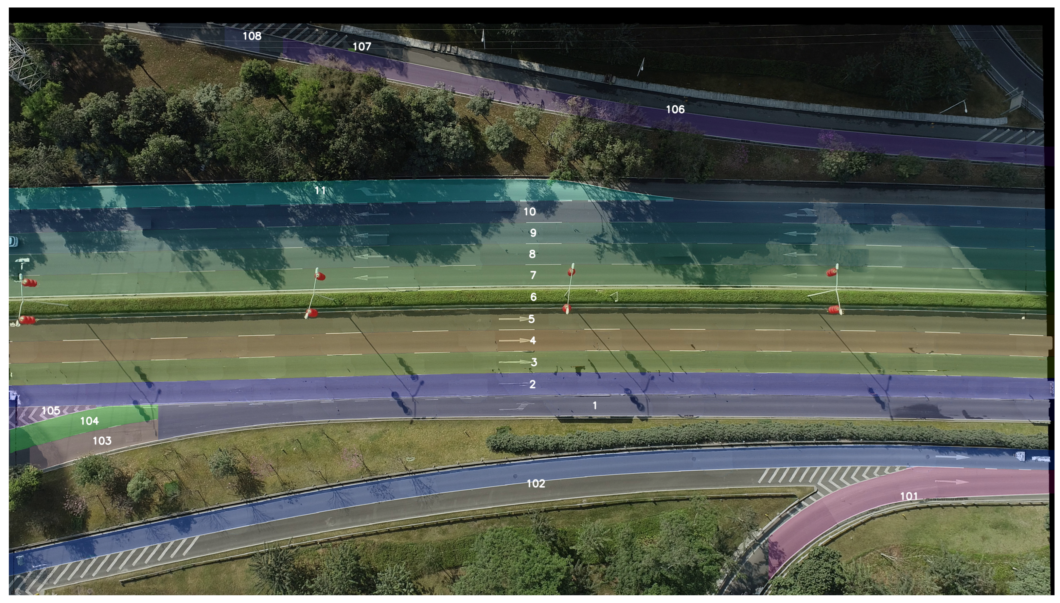
As shown in Figure 1, in the DJI dataset, the world coordinate system aligns with the image coordinate system used for video recording. The origin of the image coordinate system is the top-left corner of the image. The horizontal axis represents the x-axis, which corresponds to the direction of vehicle travel and increases toward the right. The vertical axis represents the y-axis, which increases downward. In the image coordinate system, the (x, y) coordinates of the vehicle trajectory represent the position of the center point of the vehicle’s bounding box.

In this study, vehicle trajectory coordinates were processed according to the image coordinate system used for video recording. We used these processed coordinates as both input and ground truth for the network.

2.3. Data Preparation

A first-order Savitzky–Golay filter with a short window size was applied to smooth the longitudinal and lateral coordinates of the trajectories. This was necessary because the DJI dataset, derived from video-based tracking, may suffer from detection dropouts or tracking inconsistencies caused by occlusions, missed detections, or visual ambiguity. The filtering process improves temporal continuity, allowing the model to capture coherent motion patterns without being misled by such artifacts. In addition, we assumed that predicting the motion of surrounding vehicles could be based primarily on the motion data of these vehicles collected by the autonomous vehicle, with minimal reliance on additional information from the traffic scene, such as the positions of other traffic participants and road conditions. In practical applications, this method offers two primary advantages. First, the need for extensive data collection on other vehicle information is reduced, consequently reducing the computational burden on autonomous vehicles. Second, the randomness of vehicle motion intentions is comprehensively considered without depending on the game-theoretic relationships of other traffic participants.

2.4. Features

In this section, the principle guiding the selection of data features is that they should pertain to vehicle motion intentions and be readily obtainable through vehicle-mounted sensors such as LiDAR, millimeter-wave radar, and cameras. Thus, the following vehicle motion features are defined for the input data:

• Longitudinal coordinate: x in the image coordinate system;
• Lateral coordinate: y in the image coordinate system;
• Longitudinal velocity: x velocity;
• Lateral velocity: y velocity;
• Longitudinal acceleration: x acceleration;
• Lateral acceleration: y acceleration;
• Driving direction: orientation;
• Centerline offset: ego_offset, which is the offset of the vehicle center point from the current lane centerline.

These data features were selected based on the following rationale: vehicle trajectory coordinates at historical time steps establish the starting point for predicting future trajectories; longitudinal and lateral velocities directly influence changes in the vehicle’s trajectory, whereas acceleration indicates the vehicle’s earlier motion trend; lastly, the driving direction and ego offset are associated with vehicle lane-changing intentions. A two-step scaling process on the vehicle trajectory coordinates $(x,y)$ was performed considering the characteristics of the activation functions. First, the initial frame vehicle coordinates of each sample data as the origin were used to calculate the relative driving trajectory $(x^{\prime },y^{\prime })$. Next, the mean and standard deviation of the values in the dataset were calculated for each feature dimension of the input data, and each feature dimension was standardized.

This study aims to predict the future potential occupancy set of vehicles. The ground truth features of the output data were defined as the centerline coordinates of the occupancy set, and other vehicle motion information was ignored. To better represent the output data, the ground truth output vector was defined as ${[xt,yt]}_{t=1\dots t_{pre}}$, which contains the values for the next k seconds. Similar to the input data, the same data processing methods were applied to the ground truth data.

3. Proposed Model

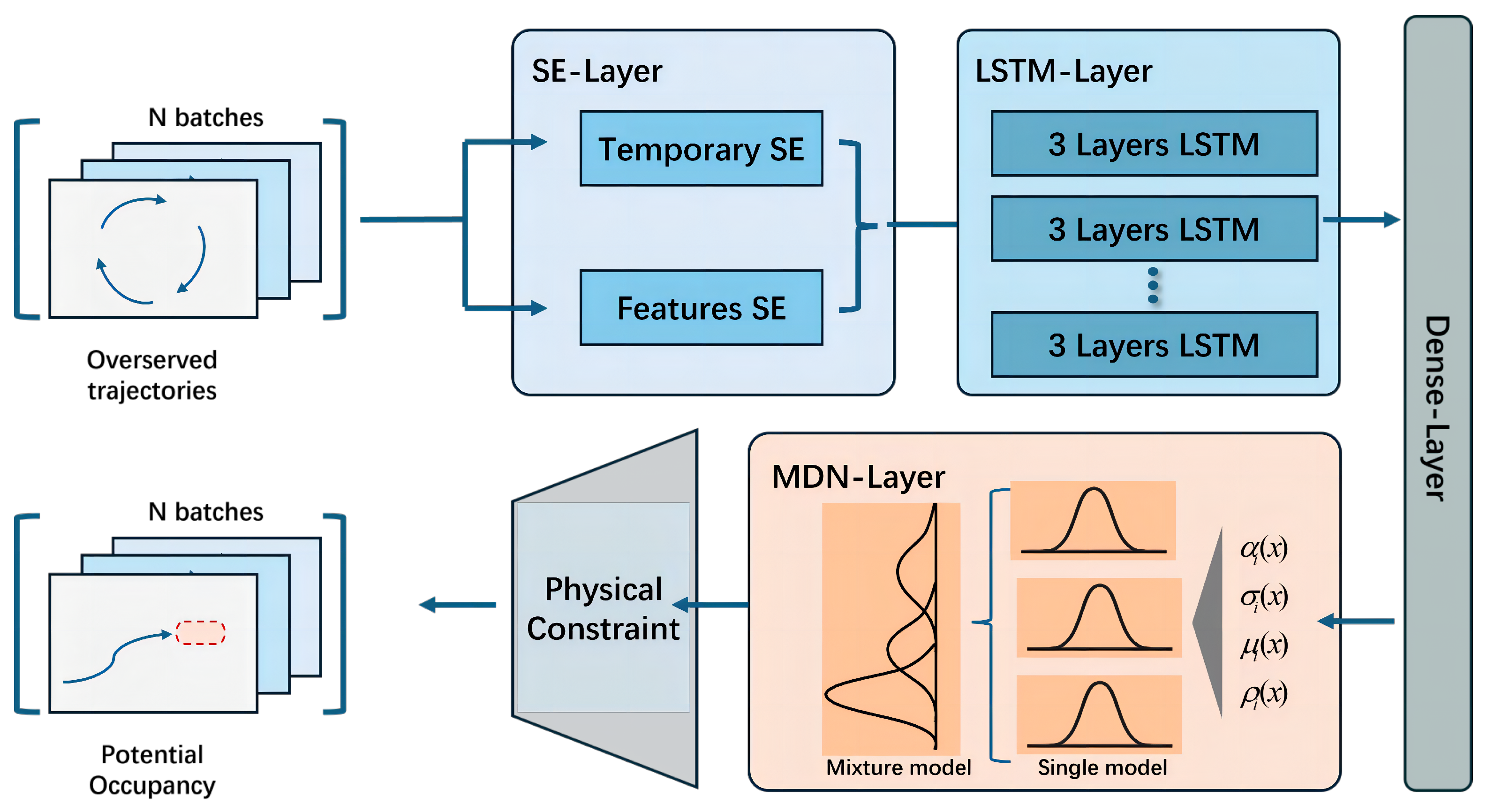
This study employs a hybrid network composed of four functional layers, as illustrated in Figure 2. The architecture includes a dual SE attention layer to highlight feature importance, an LSTM layer to capture temporal dependencies, a fully connected layer to generate MDN parameters, and an MDN layer that models multimodal distributions and quantifies prediction uncertainty. To further enhance reliability and ensure physically plausible predictions, physical constraints are also incorporated. Each layer will be described in detail in the following subsections.

3.1. Dual Squeeze-and-Excitation Layer

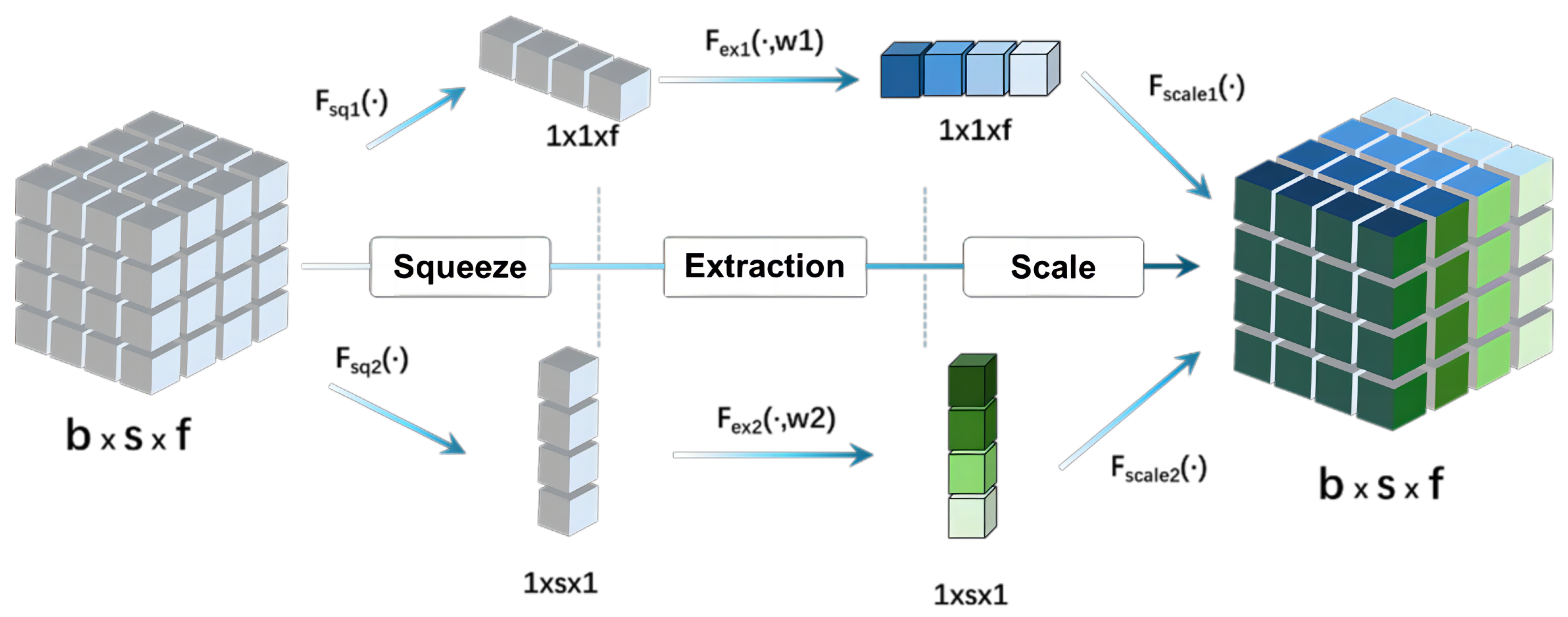
To further enhance the network’s predictive capability and improve the accuracy of trajectory prediction, a dual SE layer based on SE networks was incorporated into the first layer of the network, as shown in Figure 3. The SE network, first introduced by Hu et al., aims to improve the dependency between feature channels in convolutional neural networks [25]. Its main concept is to enhance network performance by employing an attention mechanism that computes the weight of each input channel adaptively.

In this study, two main objectives were achieved by training the dual SE layer: first, to capture the significance of various feature channels, thereby enhancing the expression capability for crucial features, and second, to understand the relevance of input information across different time points, thereby bolstering the ability of next-layer LSTM to capture relationships within the time series. The SE network structure comprises three primary operations: squeeze, excitation, and calibration.

The squeeze operation generates global feature values for each dimension by performing global average pooling on different dimensions of the input. In this context, the squeeze operation is applied separately to the time series and the feature value dimensions of the input. Global information can be extracted from the time series and feature value dimensions by performing dual compression through the dual SE module:

$$z_{\mathrm{seq}.}=F_{\mathrm{seq}.}\left(x_{\mathrm{seq}.}\right)={\displaystyle \frac{1}{H\times W}}\sum _{i=1}^H\sum _{j=1}^W{x}_{\mathrm{seq}.}(i,j)$$

(3)

$$z_{\mathrm{fea}.}=F_{\mathrm{fea}.}\left(x_{\mathrm{fea}.}\right)={\displaystyle \frac{1}{M\times L}}\sum _{i=1}^M\sum _{j=1}^L{x}_{\mathrm{fea}.}(i,j)$$

(4)

where $x_{seq.}$ denotes the information carried by each frame in the time series, and H and W represent the width and height of the input information vector for each frame, respectively. Similarly, $x_{fea.}$ is the information carried by each feature value in the time series, and $M,L$ represent the width and height of the time series information vector for each feature value, respectively.

These global features are learned through a fully connected neural network in the excitation operation, which typically comprises two fully connected layers. In the first layer, the ReLU activation function is used, and in the second layer, the Sigmoid activation function is employed. This process generates weights for each channel, indicating the importance of each respective channel:

$$s_{seq.}=F_{ex1}(z_{seq.},{W_1}_{,1})=\psi \left(g_1(z_{seq.},W_{1,1})\right)=\psi \left(W_{1,2}\delta \left(W_{1,1}{z}_{seq.}\right)\right)$$

(5)

$$s_{fea.}=F_{ex2}(z_{fea.},{W_2}_{,1})=\psi \left(g_2(z_{fea.},W_{2,1})\right)=\psi \left(W_{2,2}\delta \left(W_{2,1}{z}_{fea.}\right)\right)$$

(6)

where $\psi$ is the Sigmoid activation function, $\delta$ denotes the ReLU activation function, and $W_{1,1},W_{1,2},W_{2,1},$ and $W_{2,2}$ represent the weights of the fully connected layers corresponding to different input dimensions.

Finally, these weights are reassigned to each channel of the input feature map in the calibration operation. This involves multiplying the feature map of each channel by its corresponding weight to enhance features at the channel level:

$$\tilde{x}=F_{scale1,scale2}(x,s_{seq.},s_{fea.})=s_{seq.}·x·s_{fea.}$$

(7)

where $s_{seq.}$ and $s_{fea.}$ represent the weights for different time series and features, respectively, and $\tilde{x}$ is the recalibrated input information.

3.2. Long Short-Term Memory Layer

For output prediction, we employed a standard 3-layer LSTM network with 300 units per layer to model temporal dependencies in the input sequences. LSTM was selected due to its proven effectiveness in capturing long-term patterns in sequential data and its robustness in training stability.

3.3. Mixture Density Network Layer

An MDN was added following the LSTM layer of the network to better fit the multimodal nature of the data and quantify the uncertainty of the prediction results. This network integrates a GMM with a neural network, enabling the quantification of model uncertainty in the form of a probability density. In contrast to the fully connected layer of a typical neural network, the MDN does not treat the network’s output values directly as predictions. Instead, each output value is considered a mixture of Gaussian distributions rather than a deterministic value or a single Gaussian distribution [26]. The GMM effectively addresses the drawbacks of a single Gaussian distribution when dealing with multivalued mapping problems, thereby improving the accuracy in capturing the complex characteristics and uncertainties of the data. 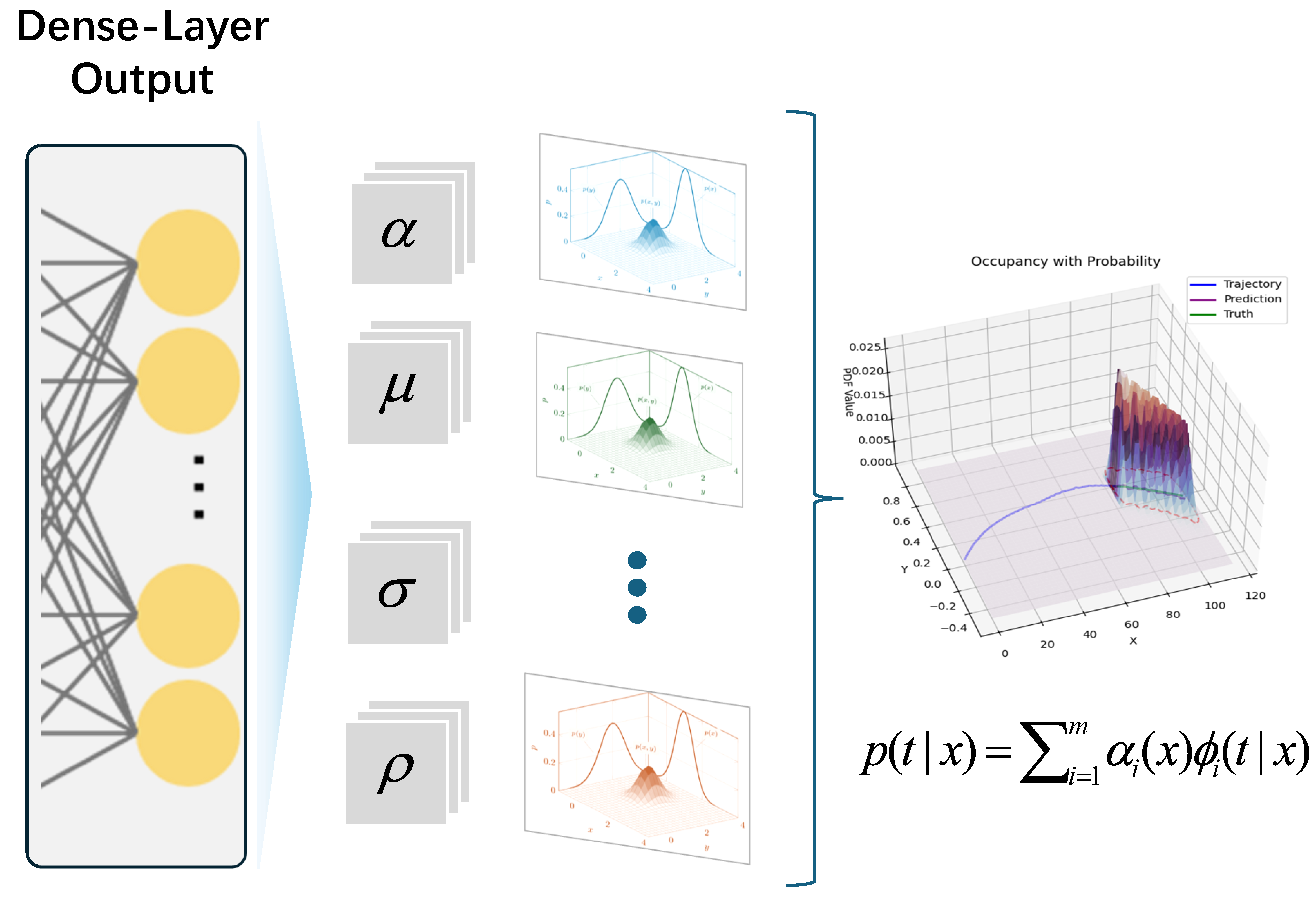Figure 4 illustrates the architecture of the MDN.

Consider X as the input and $\theta$ as the output, where the input and output can be vectors of multiple dimensions. We can express the probability density of the target value as a linear combination of multiple kernel functions:

$$p\left(\theta \right|x)={\sum }_{i=1}^m{\alpha }_i\left(x\right){\varphi }_i\left(\theta \right|x)$$

(8)

where ${\alpha }_i\left(x\right)$ is the mixing coefficients, ${\varphi }_i$ represents the i-th kernel of the target vector $\theta$, and there are m kernels in total. These kernel functions can theoretically be any probability distribution function. Considering the Gaussian distribution’s excellent fitting properties and the requirement that the prediction output in this study consists of the future occupancy set with two feature values (longitudinal and lateral coordinates), the bivariate Gaussian distribution function was selected as the kernel function.

By substituting the bivariate Gaussian distribution formula, we can express the MDN probability density function as

$$\begin{array}{cc}\hfill p(x,y|X)=& \sum _{i=1}^m{\alpha }_i\left(X\right){\displaystyle \frac{1}{2\pi {\sigma }_{x_i}\left(X\right){\sigma }_{y_i}\left(X\right)\sqrt{1-{\rho }_i{\left(X\right)}^2}}}\hfill \\ \hfill & \times exp\left(-{\displaystyle \frac{1}{2(1-{\rho }_i{\left(X\right)}^2)}}\left[{\left({\displaystyle \frac{x-{\mu }_{x_i}\left(X\right)}{{\sigma }_{x_i}\left(X\right)}}\right)}^2+{\left({\displaystyle \frac{y-{\mu }_{y_i}\left(X\right)}{{\sigma }_{y_i}\left(X\right)}}\right)}^2\right.\right.\hfill \\ \hfill & \left.\left.-{\displaystyle \frac{2{\rho }_i\left(X\right)(x-{\mu }_{x_i}\left(X\right))(y-{\mu }_{y_i}\left(X\right))}{{\sigma }_{x_i}\left(X\right){\sigma }_{y_i}\left(X\right)}}\right]\right)\hfill \end{array}$$

(9)

In neural networks, the variables to be optimized are the parameters ${\alpha }_i\left(X\right)$, ${\mu }_{x_i}\left(X\right)$, ${\mu }_{y_i}\left(X\right){\sigma }_{x_i}\left(X\right)$, ${\sigma }_{y_i}\left(X\right),$ and ${\rho }_i\left(X\right)$ in the above formula.

In the neural network, the SoftMax function is used to calculate the mixing coefficients ${\alpha }_i\left(X\right)$:

$${\alpha }_i={\displaystyle \frac{exp\left(z_i^{\alpha }\right)}{{\sum }_{j=1}^{M}exp\left(z_j^{\alpha }\right)}}$$

(10)

where $z_i^{\alpha }$ represents an output variable of the neural network. Similarly, we can express the variance and mean of each Gaussian component as

$${\sigma }_{x_i}=exp\left(z_i^{\sigma }\right)$$

(11)

$${\sigma }_{y_i}=exp\left(z_i^{\sigma }\right)$$

(12)

$${\mu }_{x_i}=z_{x_i}^{\mu }$$

(13)

$${\mu }_{y_i}=z_{y_i}^{\mu }$$

(14)

Given that the output comprises two features and no assumptions are made about the relationship between these two feature variables, the neural network must estimate the off-diagonal elements of the covariance matrix. Since these values fall within the range $[-1,1]$, their estimated values are represented as follows:

$${\rho }_i=tanh\left(z_i^{\rho }\right)$$

(15)

To facilitate a better comparison between the predicted and actual results, an additional output of the MDN layer representing the centerline of the occupancy set was included, expressed as

$${\mu }_{center}=\sum _{i=1}^m{\alpha }_i({\mu }_{x_i},{\mu }_{y_i})$$

(16)

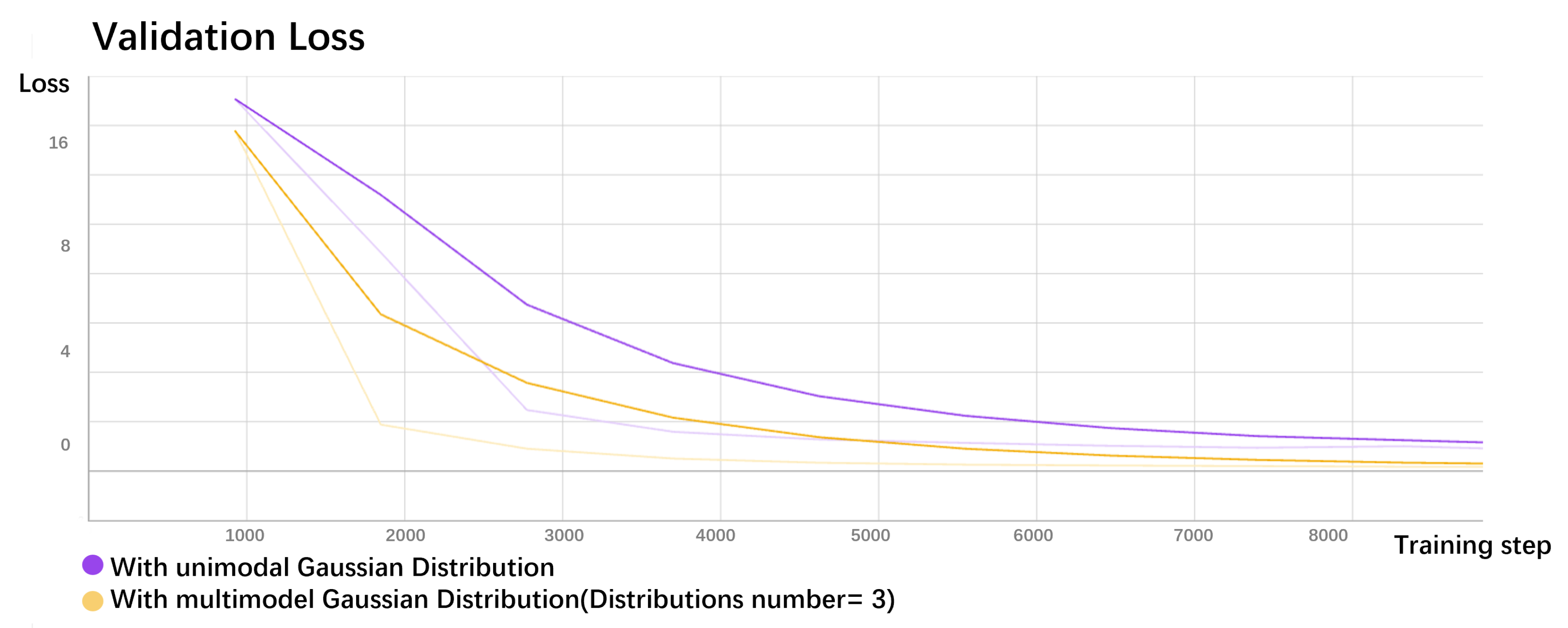
The likelihood function is defined as the loss function of the MDN. Given the parameters, we aim to determine the optimal values that maximize $p(x,y|\mathbf{x})$. The loss function is expressed as follows:

$${\mathcal{L}}_{MDN}=\sum _q{\mathcal{L}}^q$$

(17)

$${\mathcal{L}}^q=-log\left\{\sum _{i=1}^m{\alpha }_i\left(x^q\right){\varphi }_i\left({\theta }^q|x^q\right)\right\}$$

(18)

where q represents the loss value at the q-th frame.

The neural network can optimize the parameters to fit the data distribution and quantify the uncertainty accurately by minimizing this error function.

3.4. Physical Constraint

To enhance the reasonableness and stability of the model’s predictions, physical constraints were introduced. The mean of the Gaussian mixture distribution was computed to establish the centerline of the occupancy set. These physical constraints are primarily reflected in two aspects: endpoint constraints and trajectory constraints of the centerline.

First, the constraints on the starting and ending points of the predicted trajectory were considered to ensure that the predicted trajectory closely covered the actual trajectory:

$$L_{endp\mathrm{o}\mathrm{int}}=Loss(Y_{end},Y_{start},{\widehat{Y}}_{end},{\widehat{Y}}_{start})$$

(19)

where $Loss$ represents the loss function, $Y_{end},Y_{start}$ represents the endpoint coordinates of the actual values, and ${\widehat{Y}}_{end},{\widehat{Y}}_{start}$ are the coordinates of the centerline predicted by the model.

Furthermore, constraints were imposed on the lateral shifts of the centerline, and the oscillations in the lateral trajectory were restricted. To limit significant changes in the lateral translation of the centerline, the difference in the longitudinal position of adjacent points, $x_{diff,i}=x_i-x_{i-1}$, was calculated. The minimum displacement $x_{min\_movement}$ was defined as the kinematic constraint value. Similarly, to restrict oscillations in the lateral position, the difference in lateral positions $y_{diff,i}=y_i-y_{i-1}$ was calculated, and the maximum jump per unit distance $y_{max\_jump}$ was defined.

$$L_{trajectory}=Loss(x_{diff},x_{min\_movement})+Loss(y_{diff},y_{max\_jump})$$

(20)

where $Loss$ represents the loss function employed for the physical constraints. The expression of the final physical constraints is as follows:

$$L_{physical}=L_{endpo\mathrm{int}}+L_{trajectory}$$

(21)

The reasonableness of the model’s predictions can be further ensured by applying these physical constraints.

4. Experiment

4.1. Training Step

In this section, based on the sampled data from the AD4CHE dataset, the previously described hybrid network that was used to predict the future potential occupancy sets of surrounding vehicles is presented. Figure 2 shows the overall network structure. This study aims to design a network that can understand 10 s of historical data to predict the occupancy set for the next 3 s. Given that the DJI dataset has a sampling frequency of 30 Hz, a 300-input window representing 10 s of observation data was used to train the network. The subsequent 90 trajectory coordinates were used as the ground truth for the centerline distribution of the predicted occupancy set.

The training data and prediction results were grouped based on scenario numbers, leading to a total of 68 scenarios. For these data, 80% of the data from the first 54 scenarios were used as training data, and the remaining 20% from the first 54 scenarios and all data from the remaining 14 scenarios were used as test data. The test data were excluded from the training process. Consequently, for the n-th scenario, the actual data input into the network is a 3D tensor B × 300 × N, where N = 8 represents the number of features, and B denotes the total number of windows for that scenario, which varies based on the number of trajectories collected in each scenario and is not fixed. The model was trained on a GPU using the Adam optimizer with an initial learning rate of 0.002 and a batch size of 32. The model was trained on a GPU using the Adam optimizer (initial learning rate: 0.002, batch size: 32) with an adaptive scheduler that reduced the learning rate when validation loss plateaued, ensuring fast and stable convergence. The loss function used for each training sample was

$$L_{\mathit{training}}=k_1{L}_{physical}+k_2{L}_{MDN}$$

(22)

where $k_1,k_2$ represent the loss weights. To improve the interpretability of the network’s prediction results, $k_1$ was set to 10 and $k_2$ to 1 during the training process, thereby amplifying the influence of the physical constraints on the network.

4.2. Squeeze-And-Excitation Layer Validation

The effectiveness of the SE layer’s attention mechanism was verified after completing the training. As illustrated in Figure 5, the weights assigned by the SE layer to the input were visualized in the form of a matrix heatmap. In the matrix heatmap, the vertical axis represents the different features, and the horizontal axis shows the number of time frames. For better visualization, each sample’s 300-frame input was divided into six subplots.

Different weights are assigned by the SE layer to various features and time frames, directing the network’s attention to more crucial features and time frames. In terms of the time series, the attention is relatively scattered and intermittent before frame 210. Nevertheless, the attention becomes continuous after frame 210. In terms of the features, the first six features are given greater attention within the same time frame. Conversely, the last two features—vehicle driving direction and deviation from the centerline—are considered less crucial and contribute minimally. By enabling the network to focus more on essential features, the SE layer reduces the computational load on subsequent network layers, improves the training convergence of the network, and enhances computational efficiency.

4.3. Comparison Between Unimodal and Multimodal Gaussian Distributions

The impact of unimodal and multimodal Gaussian distributions on prediction accuracy was compared during the training process. A multimodal Gaussian distribution comprising a mixture of three Gaussian distributions was used in our experiments. The accuracy of the two approaches exhibited significant differences when predicting aggressive driving behaviors, particularly when the vehicle changed lanes continuously.

The unimodal prediction results indicate a significant deviation in the latter half of the occupancy set, with a decreased concentration of probability density, as shown in Figure 6. In addition, the multimodal Gaussian distribution demonstrated better convergence speed during training, with the validation loss gradient decreasing more significantly compared with the unimodal Gaussian distribution, as illustrated in Figure 7.

4.4. Result

The prediction results on the test data are presented based on the categorized vehicle behaviors. As shown in Figure 8a, the network demonstrates strong fitting performance in lane-keeping scenarios, with the actual trajectory closely aligned with the center of the predicted occupancy set. Despite an initial deviation from the centerline, the model accurately maintained the lane-keeping prediction without mistakenly forecasting a lane change, reflecting the vehicle’s true behavior.

The potential future occupancy set was generated by sampling from the mixture distribution’s probability density function, visualized as a 3D heatmap. The outer boundaries of the occupancy set correspond to a probability density value equal to $5\%$ of the distribution’s peak. The model’s performance in predicting lane changes is illustrated in Figure 8b,c, which also show strong alignment with ground truth trajectories.

Beyond these common patterns, a special case was observed where the vehicle initially intended to change lanes to the left but aborted and switched to a right lane change, as depicted in Figure 8d. This abrupt behavioral shift was also accurately captured by the model.

In Figure 8a,b,d, the peak probability density is more concentrated in the early segments of the predicted trajectories. This reflects the model’s higher confidence in short-term predictions. As prediction horizons extend, uncertainty increases, resulting in broader, flatter density distributions.

Further examining Figure 8, the predicted occupancy sets not only align with observed behaviors but also capture subtle variations. The asymmetric spread in lane-change scenarios (Figure 8b,c) indicates the model’s sensitivity to directional intent, while the accurate capture of the shift in Figure 8d highlights its responsiveness to sudden behavioral changes. These results demonstrate the model’s capacity to represent both dominant and nuanced driving intentions.

5. Conclusions

This study proposed a hybrid network for predicting the future occupancy set of vehicles. Key motion features were first extracted using a dual squeeze-and-excitation (SE) layer, followed by future trajectory prediction through an LSTM network. To enhance accuracy and quantify uncertainty, a multimodal Gaussian mixture model (GMM) was applied after the LSTM, enabling probabilistic occupancy estimation by combining multiple Gaussian components. The model was trained on the DJI AD4CHE dataset, which reflects region-specific traffic patterns under Chinese road conditions, making the approach particularly suitable for analyzing localized driving behaviors. The proposed framework shows promising potential beyond conventional path prediction, including its applicability in full self-driving (FSD) systems for assessing decision-related safety risks. Future research may further explore its integration into real-time planning modules to improve the safety performance of autonomous vehicles.

We recognize that evaluating the model under compromised input scenarios—such as GPS inaccuracies, detection failures, or occlusions—is essential for assessing its effectiveness in real-world conditions. Potential limitations may also emerge in congested traffic, abrupt maneuvers, or under significant distributional shifts. In particular, since the current framework does not explicitly model interactions between multiple agents, its performance may degrade in dense, interaction-heavy environments where mutual influence between vehicles is critical. As the model is trained solely on the AD4CHE dataset, future work will focus on extending its generalization to diverse traffic domains, improving robustness to various forms of input uncertainty, and incorporating interaction-aware mechanisms for better handling of multi-agent dynamics.