Author Contributions
Conceptualization, A.-L.L.-L., H.-G.A.-M., and E.M.-M.; Data curation, A.-L.L.-L.; Formal analysis, A.-L.L.-L.; Investigation, A.-L.L.-L.; Methodology, A.-L.L.-L., H.-G.A.-M., and E.M.-M.; Resources, A.-L.L.-L., H.-G.A.-M., and E.M.-M.; Software, A.-L.L.-L.; Supervision, H.-G.A.-M. and E.M.-M.; Validation, H.-G.A.-M. and E.M.-M.; Visualization, A.-L.L.-L.; Writing—original draft, A.-L.L.-L.; Writing—review and editing, A.-L.L.-L., H.-G.A.-M., and E.M.-M. All authors have read and agreed to the published version of the manuscript.
Figure 2.
DE algorithm with SHADE.
Figure 2.
DE algorithm with SHADE.
Figure 3.
Grayscale image.
Figure 3.
Grayscale image.
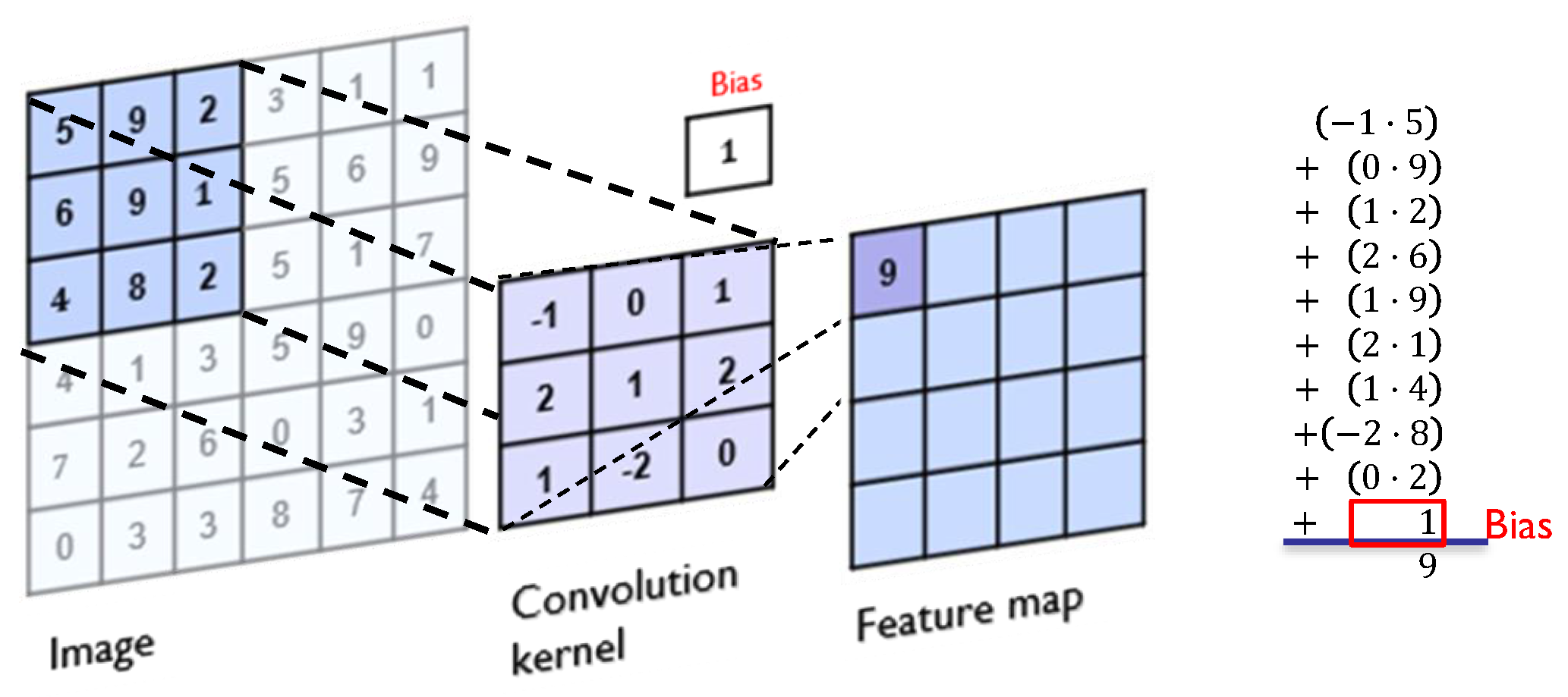
Figure 4.
Convolution process on a 6 × 6 image with a 3 × 3 kernel.
Figure 4.
Convolution process on a 6 × 6 image with a 3 × 3 kernel.
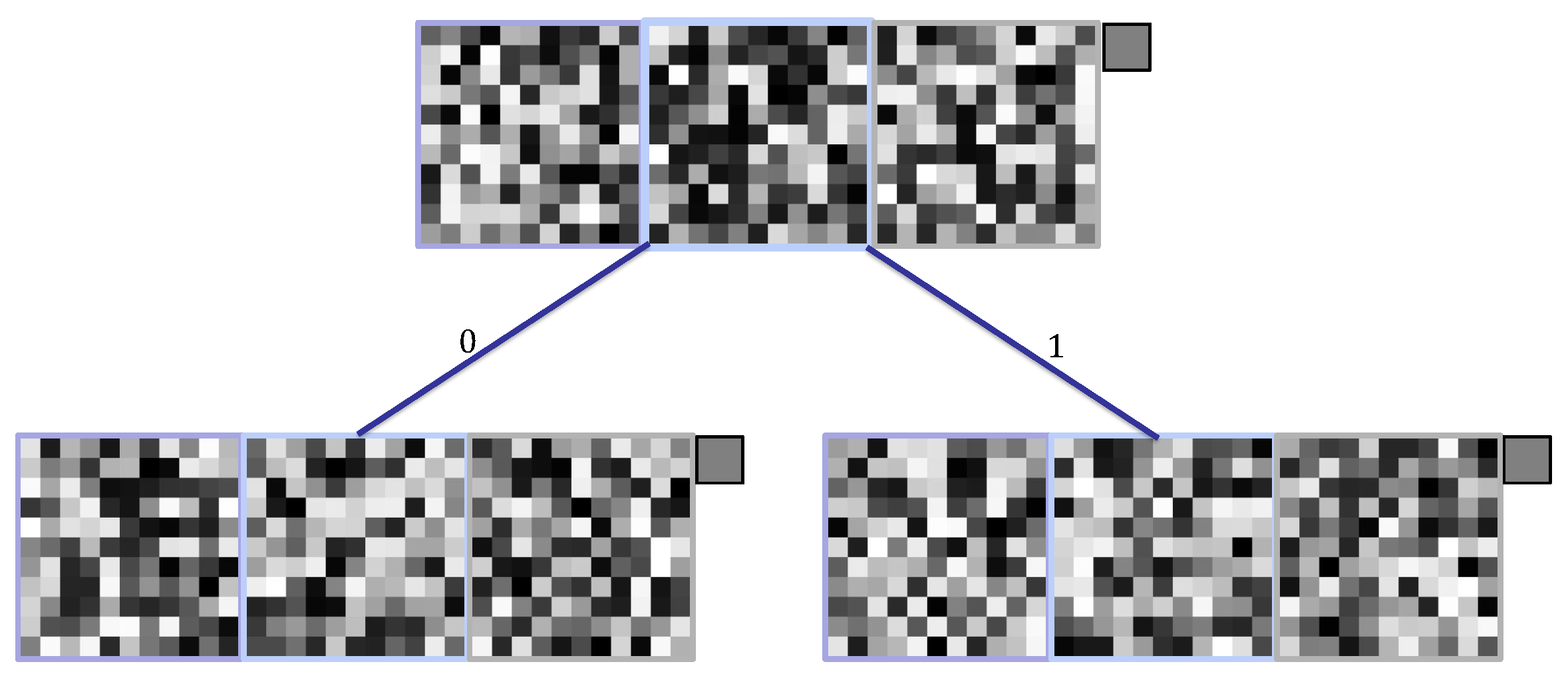
Figure 5.
Convolutional Decision Tree with kernels of size 3 and depth 2.
Figure 5.
Convolutional Decision Tree with kernels of size 3 and depth 2.
Figure 6.
Encodings of a kernel and an individual for the SHADE-CDT technique to induce a CDT of depth 3 with kernels of size 3.
Figure 6.
Encodings of a kernel and an individual for the SHADE-CDT technique to induce a CDT of depth 3 with kernels of size 3.
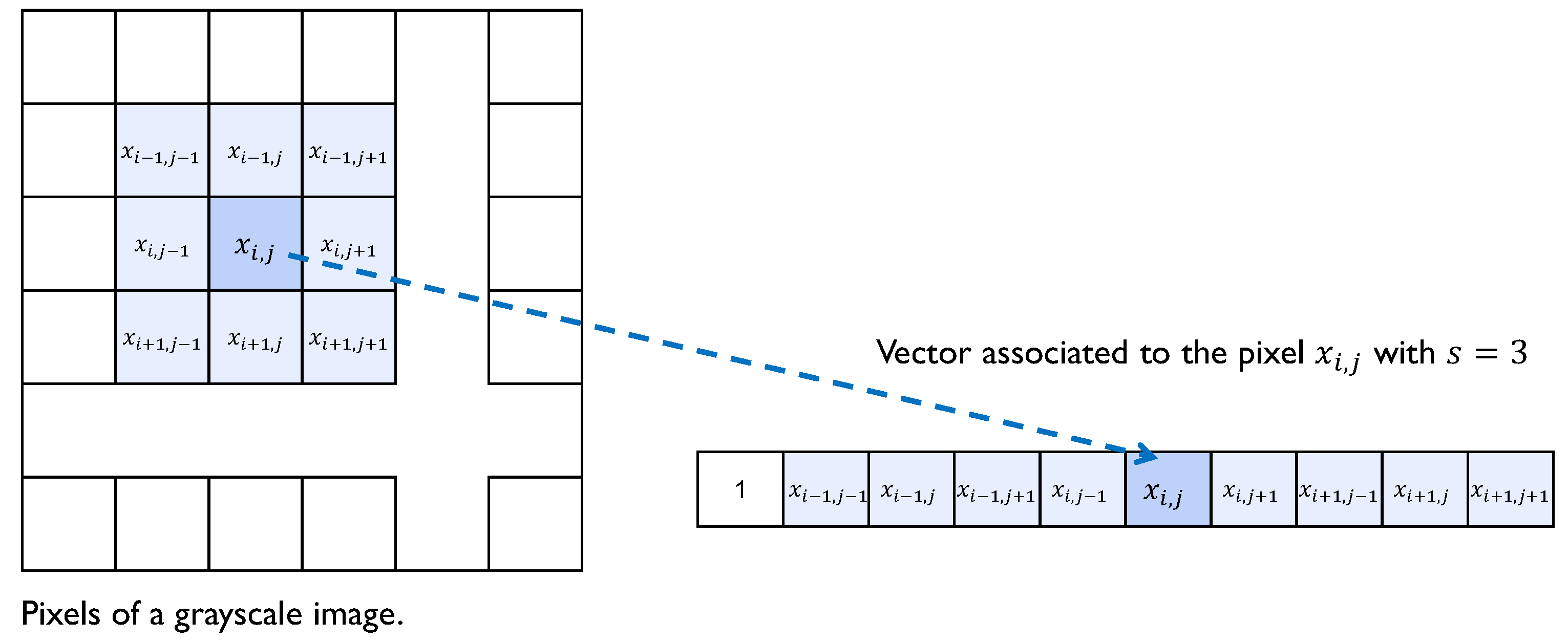
Figure 7.
Coding of a pixel-associated instance.
Figure 7.
Coding of a pixel-associated instance.
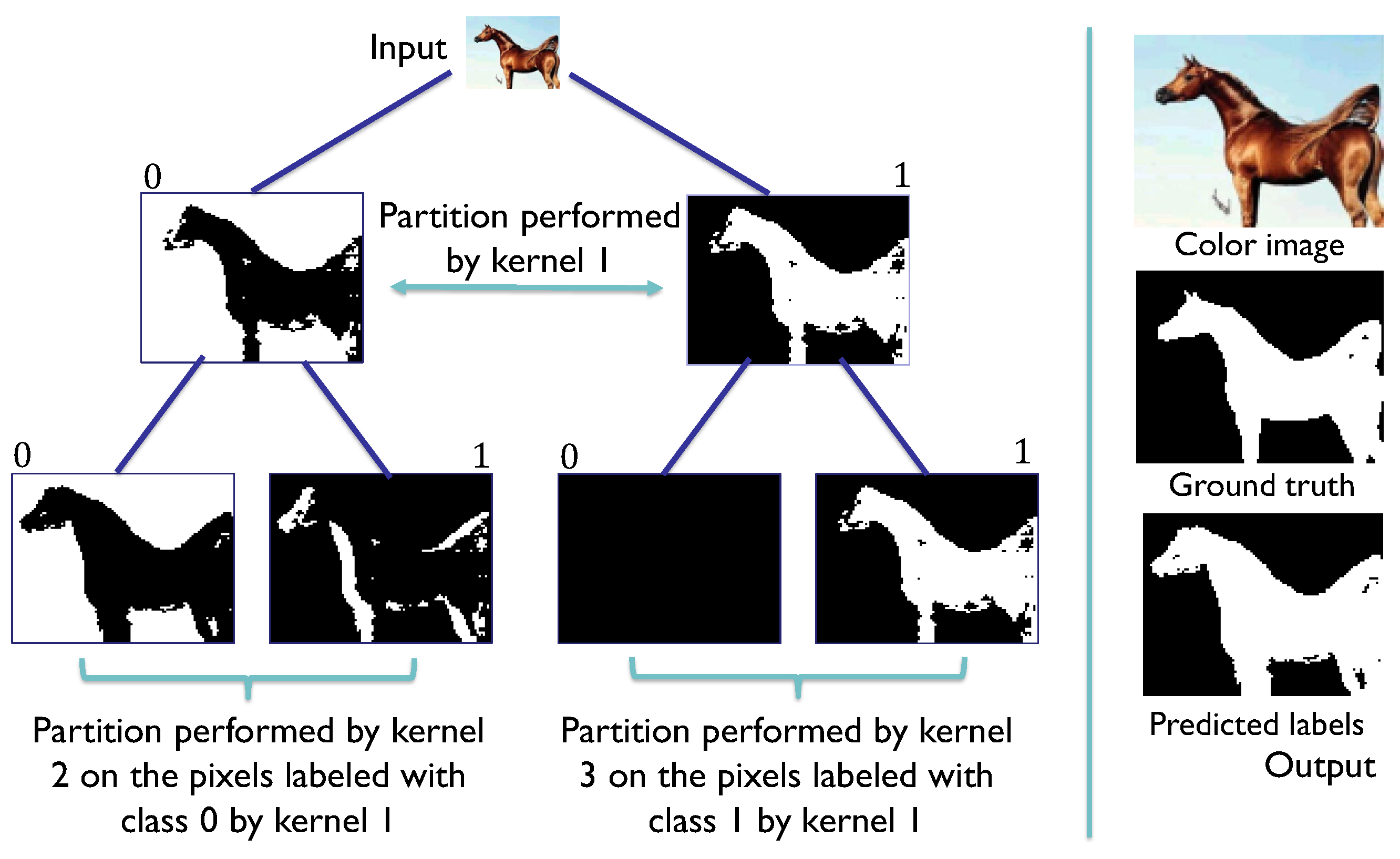
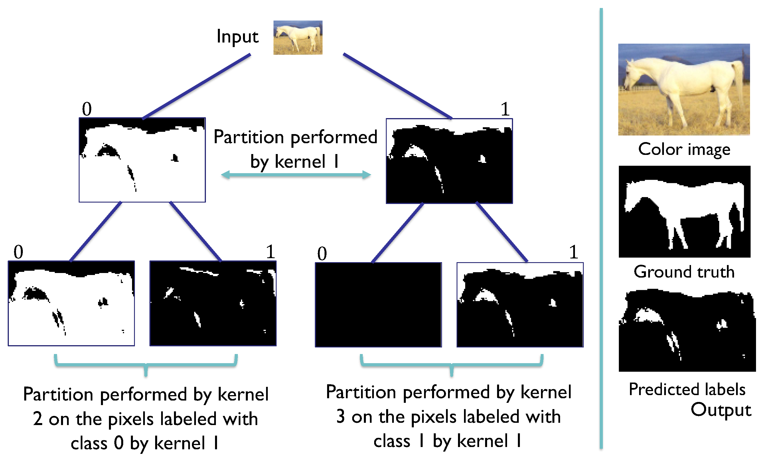
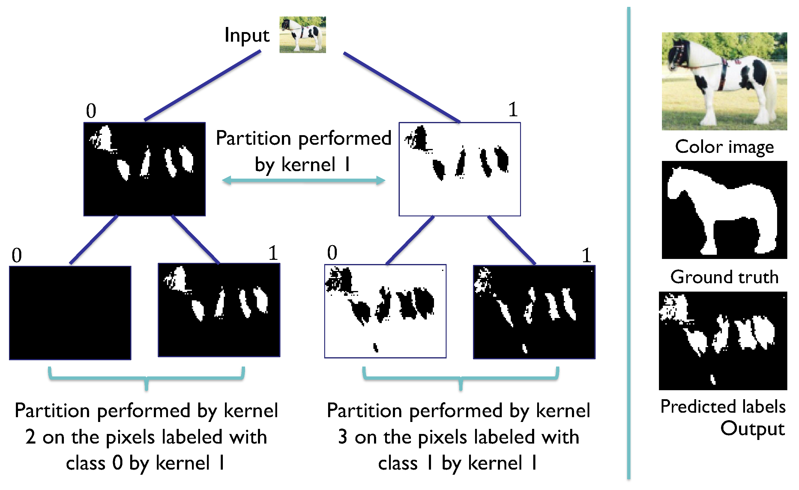
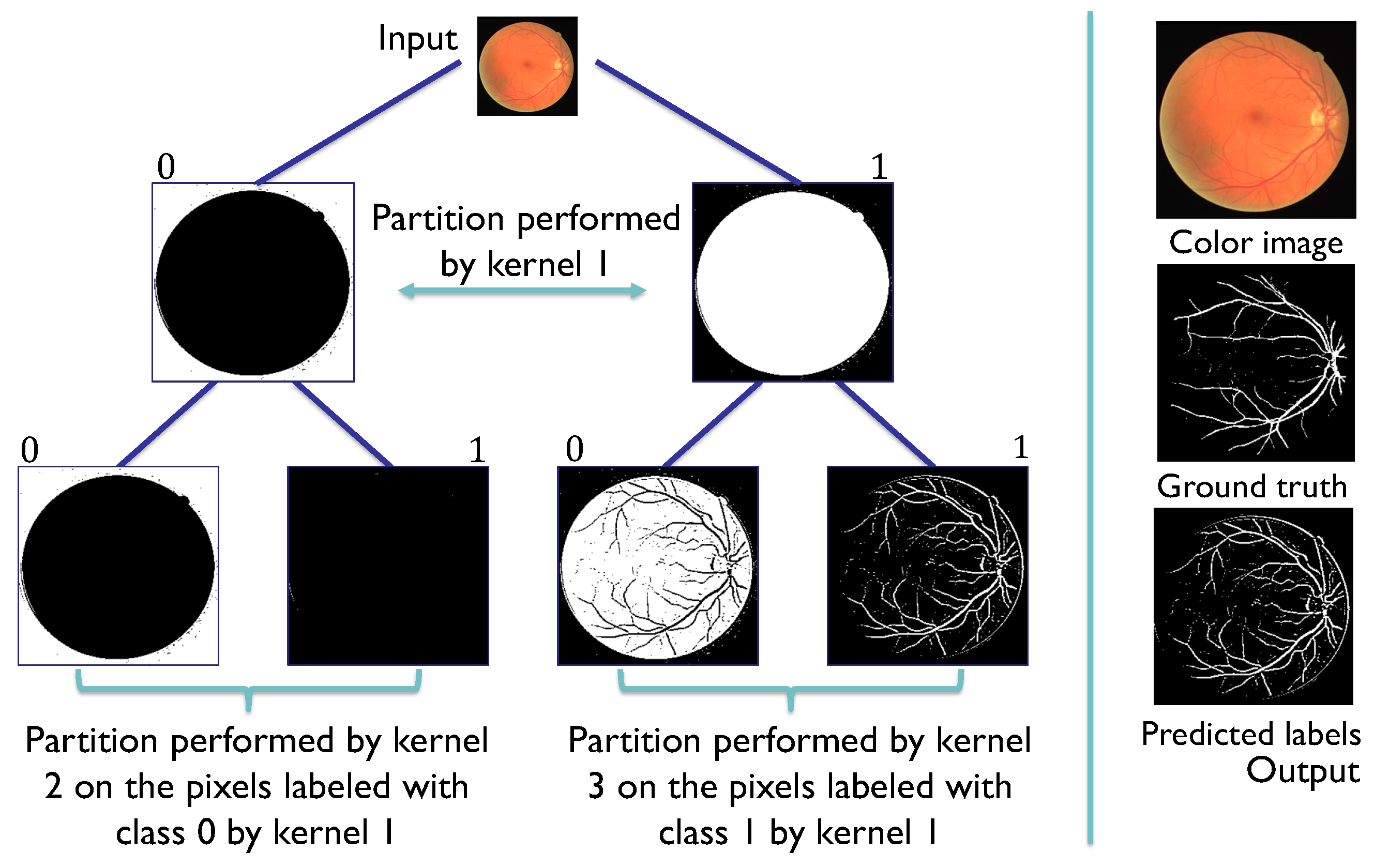
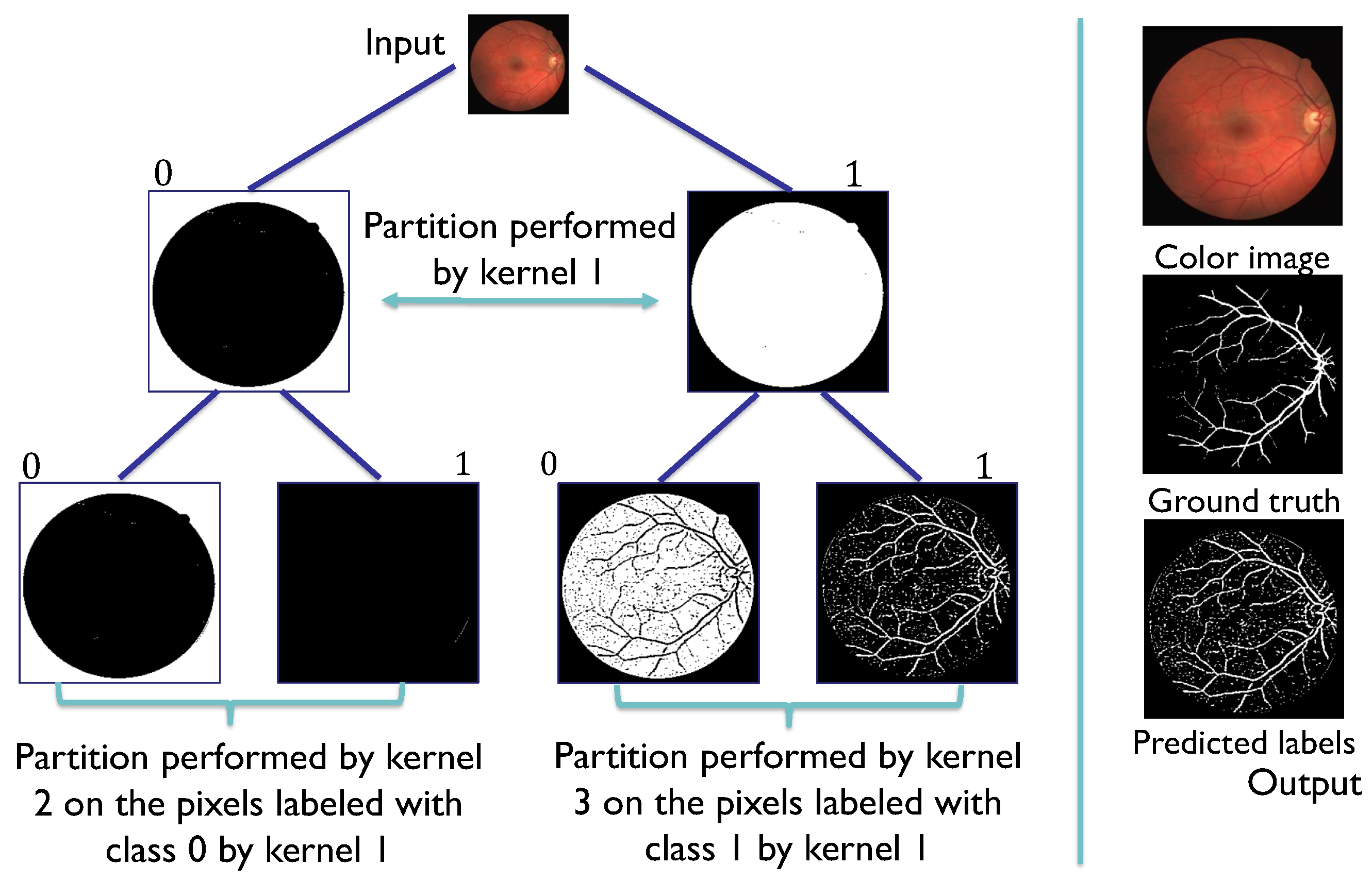
Figure 8.
SHADE-CDT process employing the codification of the pixel-associated instance (x) and the codification of the convolutional kernels (w) in the nodes of a CDT. The dot product between x and w is evaluated in the sigmoid function to obtain a value between 0 and 1. In this example, this evaluation is greater than 0.5, so the label assigned for the root node, denoted as , is 1, highlighted in the CDT, directing the pixel information to the node . The same process is repeated with the codification of node to obtain the label 0, directing the pixel information to the leaf node . With its vectorial codification, the process obtains the final label 1 for the pixel under consideration.
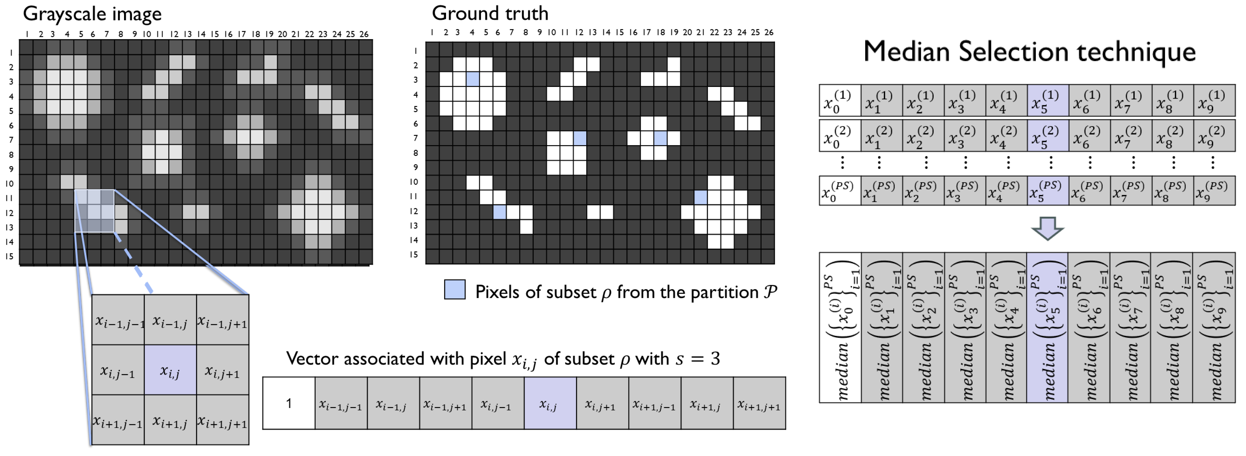
Figure 9.
Grayscale image and its ground truth on the left, and a representation of the obtention of a representative vector for the analyzed subset with the median selection technique.
Figure 9.
Grayscale image and its ground truth on the left, and a representation of the obtention of a representative vector for the analyzed subset with the median selection technique.
Figure 10.
Color spaces analyzed in this work: (a) RGB. (b) CIE L*a*b*. (c) HSV.
Figure 10.
Color spaces analyzed in this work: (a) RGB. (b) CIE L*a*b*. (c) HSV.
Figure 11.
Composition of a color image by channels.
Figure 11.
Composition of a color image by channels.
Figure 12.
convolutional kernel process on an image with three channels of color.
Figure 12.
convolutional kernel process on an image with three channels of color.
Figure 13.
Convolution process on an image with three color channels with a kernel of size .
Figure 13.
Convolution process on an image with three color channels with a kernel of size .
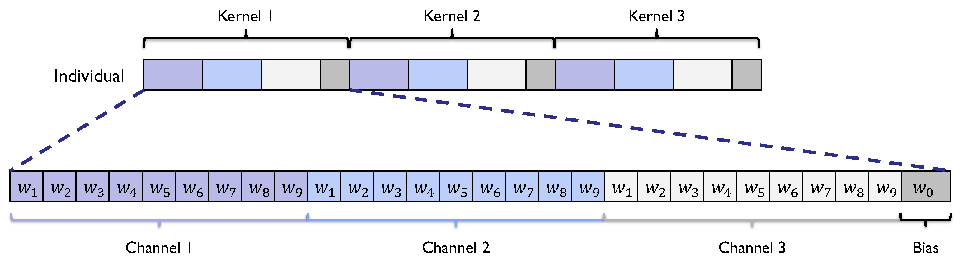
Figure 14.
Encodings of a kernel and an instance by color channel.
Figure 14.
Encodings of a kernel and an instance by color channel.
Figure 15.
Individual considered in the SHADE process for the induction of a CDT with kernel size and depth (vector of length ).
Figure 15.
Individual considered in the SHADE process for the induction of a CDT with kernel size and depth (vector of length ).
Figure 16.
Information of the pixel structured for the SHADE process considering a kernel of size .
Figure 16.
Information of the pixel structured for the SHADE process considering a kernel of size .
Figure 17.
The memory implemented for the - method calculates the fitness for all individuals in the initial population, and, for subsequent populations, only the fitness for the new individuals in the immediate next generation is calculated, reducing the computational time of the induction process.
Figure 18.
Line plots in two dimensions considering the depth d of the CDTs and their corresponding F1-scores, fixing the kernel size s. (a) CDTs with . (b) CDTs with . (c) CDTs with . (d) CDTs with . (e) CDTs with .
Figure 18.
Line plots in two dimensions considering the depth d of the CDTs and their corresponding F1-scores, fixing the kernel size s. (a) CDTs with . (b) CDTs with . (c) CDTs with . (d) CDTs with . (e) CDTs with .
Figure 19.
Boxplots of the F1-scores obtained in five experiments in each color space and in each of the following CDT structures: (a) CDTs with and . (b) CDTs with and . (c) CDTs with and . (d) CDTs with and . (e) CDTs with and .
Figure 19.
Boxplots of the F1-scores obtained in five experiments in each color space and in each of the following CDT structures: (a) CDTs with and . (b) CDTs with and . (c) CDTs with and . (d) CDTs with and . (e) CDTs with and .
Figure 20.
Multiple comparison test between the color spaces analyzed in each of the following CDT structures: (a) CDTs with and . (b) CDTs with and . (c) CDTs with and . (d) CDTs with and . (e) CDTs with and .
Figure 20.
Multiple comparison test between the color spaces analyzed in each of the following CDT structures: (a) CDTs with and . (b) CDTs with and . (c) CDTs with and . (d) CDTs with and . (e) CDTs with and .
Figure 21.
Spider graph of the results obtained with the three analyzed color spaces (RGB, CIE L*a*b*, and HSV) and the different CDT structures (kernel size s and depth d). Value 1 indicates that the color space has obtained the best segmentation result in the corresponding CDT structure. Value of 0 indicates the contrary case.
Figure 22.
Plot line to compare the F1-scores and the induction time results with each method (- and -), indicating the kernel size s considered on each point.
Figure 22.
Plot line to compare the F1-scores and the induction time results with each method (- and -), indicating the kernel size s considered on each point.
Table 1.
Computer specifications.
Table 1.
Computer specifications.
| Operating System | Windows 11 Pro 23H2 |
| RAM | 64 GB |
| Processor | AMD Ryzen 5 5600G |
| Processor speed | 3.90 GHz |
Table 2.
Results for the Weizmann Horse dataset segmentation with the - method employing the median technique with , and, for the SHADE algorithm, 100 individuals, 100 generations, and a memory size of 100. The best F1-score by kernel size, considering the color space, is shown in bold numbers, and the best result by kernel size is highlighted.
| CDT Structure | RGB | CIE L*a*b* | HSV |
|---|
| | F1-Score | Accuracy | Time (min) | F1-Score | Accuracy | Time (min) | F1-Score | Accuracy | Time (min) |
| 3 | 1 | 0.5415 | 0.7632 | 6.39 | 0.5466 | 0.7653 | 6.18 | 0.3996 | 0.7383 | 6.64 |
| 3 | 2 | 0.5346 | 0.7509 | 10.6 | 0.548 | 0.7645 | 10.44 | 0.5239 | 0.7675 | 10.82 |
| 3 | 3 | 0.5718 | 0.773 | 14.23 | 0.5654 | 0.7664 | 14.27 | 0.5143 | 0.7692 | 14.36 |
| 3 | 4 | 0.5534 | 0.7492 | 18.08 | 0.5689 | 0.7692 | 18.25 | 0.5353 | 0.7623 | 18.7 |
| 3 | 5 | 0.5664 | 0.7669 | 22.39 | 0.5664 | 0.7648 | 24.62 | 0.5455 | 0.7689 | 22.16 |
| 5 | 1 | 0.5562 | 0.7702 | 7.26 | 0.5567 | 0.7647 | 7.16 | 0.4087 | 0.7331 | 6.65 |
| 5 | 2 | 0.5544 | 0.7694 | 11.22 | 0.581 | 0.76 | 11.37 | 0.4966 | 0.7457 | 11.72 |
| 5 | 3 | 0.5769 | 0.7484 | 15.41 | 0.5686 | 0.7528 | 15.68 | 0.5152 | 0.7484 | 15.81 |
| 5 | 4 | 0.5793 | 0.7502 | 19.58 | 0.593 | 0.7778 | 20.13 | 0.5359 | 0.7486 | 19.33 |
| 5 | 5 | 0.5666 | 0.7557 | 23.6 | 0.592 | 0.7703 | 24.91 | 0.512 | 0.7528 | 23.04 |
| 7 | 1 | 0.563 | 0.7689 | 8.51 | 0.5641 | 0.7635 | 8.83 | 0.4127 | 0.7235 | 8.61 |
| 7 | 2 | 0.5669 | 0.7694 | 13.25 | 0.5942 | 0.7667 | 13.22 | 0.5115 | 0.7425 | 13.82 |
| 7 | 3 | 0.5825 | 0.7532 | 18.16 | 0.5923 | 0.7672 | 17.30 | 0.5226 | 0.7513 | 18.46 |
| 7 | 4 | 0.5918 | 0.7567 | 22.76 | 0.5865 | 0.756 | 23.15 | 0.5312 | 0.7363 | 21.79 |
| 7 | 5 | 0.5671 | 0.74 | 28.09 | 0.5642 | 0.7385 | 26.13 | 0.5275 | 0.7337 | 26.44 |
| 9 | 1 | 0.5548 | 0.7586 | 11.8 | 0.5707 | 0.7631 | 11.62 | 0.4387 | 0.7183 | 11.23 |
| 9 | 2 | 0.5946 | 0.7502 | 18.38 | 0.6042 | 0.769 | 17.8 | 0.5063 | 0.7258 | 16.75 |
| 9 | 3 | 0.5936 | 0.7545 | 24.48 | 0.5897 | 0.7567 | 21.91 | 0.5214 | 0.7202 | 22.22 |
| 9 | 4 | 0.5898 | 0.7503 | 31.26 | 0.5699 | 0.7441 | 26.69 | 0.53 | 0.7376 | 29.41 |
| 9 | 5 | 0.5848 | 0.758 | 32.14 | 0.5915 | 0.7648 | 31.98 | 0.5234 | 0.7012 | 32.31 |
| 11 | 1 | 0.5559 | 0.7519 | 12.62 | 0.5806 | 0.763 | 12.43 | 0.4407 | 0.7134 | 15.09 |
| 11 | 2 | 0.5503 | 0.7458 | 19.69 | 0.6052 | 0.7585 | 18.26 | 0.5088 | 0.7129 | 20.65 |
| 11 | 3 | 0.5891 | 0.7393 | 23.71 | 0.5903 | 0.7591 | 23.68 | 0.5225 | 0.7166 | 25.76 |
| 11 | 4 | 0.5623 | 0.7411 | 29.76 | 0.5954 | 0.7507 | 28.39 | 0.5255 | 0.7179 | 30.07 |
| 11 | 5 | 0.5749 | 0.7437 | 35.69 | 0.5624 | 0.7354 | 35.64 | 0.5315 | 0.7118 | 35.49 |
Table 3.
Results of 5 experiments with the Weizmann Horse dataset in the three color spaces employing the median technique with , and for the SHADE algorithm 100 individuals, 100 generations, and a memory size of 100. The table presents the minimum, maximum, mean ± standard deviation, and median of the F1-scores obtained in each color space and with the specified CDT structure. Additionally, the mean time and two p-values for the statistical tests, namely the Shapiro–Wilk test and the one-way ANOVA test, are included, with a significance level of applied to all tests. The values in bold represent the results with the best segmentation, with two highlighted values when the differences between the corresponding color spaces are not statistically significant.
| CDT Structure | Metrics | RGB | CIE L*a*b* | HSV |
|---|
| | Min/Max | 0.5445/0.5777 | 0.5654/0.5843 | 0.5143/0.5416 |
| Mean ± St.D. | 0.5612 ± 0.0143 | 0.5714 ± 0.0075 | 0.5276 ± 0.0103 |
| Median | 0.5627 | 0.5697 | 0.5288 |
| | Time (min) | 15.81 | 15.4 | 14.48 |
| Shapiro–Wilk | p-value | 0.6189 | 0.0660 | 0.9871 |
| One-way ANOVA | p-value | | * | |
| | Min/Max | 0.5462/0.5793 | 0.5723/0.5930 | 0.5028/0.5386 |
| Mean ± St.D. | 0.5678 ± 0.0133 | 0.5823 ± 0.0075 | 0.5246 ± 0.0150 |
| Median | 0.5706 | 0.5817 | 0.5297 |
| | Time (min) | 21.31 | 21.15 | 19.54 |
| Shapiro–Wilk | p-value | 0.3067 | 0.9548 | 0.4637 |
| One-way ANOVA | p-value | | * | |
| | Min/Max | 0.5562/0.5845 | 0.591/0.6057 | 0.5023/0.5119 |
| Mean ± St.D. | 0.5660 ± 0.011 | 0.598 ± 0.006 | 0.5077 ± 0.0041 |
| Median | 0.5615 | 0.5966 | 0.5078 |
| | Time (min) | 14.5 | 14.33 | 13.7 |
| Shapiro–Wilk | p-value | 0.1777 | 0.7977 | 0.5394 |
| One-way ANOVA | p-value | | * | |
| | Min/Max | 0.5559/0.5946 | 0.5699/0.6064 | 0.5063/0.5149 |
| Mean ± St.D. | 0.5819 ± 0.0152 | 0.5951 ± 0.0147 | 0.5110 ± 0.0038 |
| Median | 0.5880 | 0.5984 | 0.5101 |
| | Time | 17.68 | 17.21 | 17.42 |
| Shapiro–Wilk | p-value | 0.0952 | 0.0687 | 0.3659 |
| One-way ANOVA | p-value | | * | |
| | Min/Max | 0.5503/0.5884 | 0.5978/0.6122 | 0.4906/0.5192 |
| Mean ± St.D. | 0.5696 ± 0.0174 | 0.6041 ± 0.0054 | 0.5096 ± 0.0115 |
| Median | 0.5719 | 0.6041 | 0.5116 |
| | Time | 19.94 | 19.6 | 20.34 |
| Shapiro–Wilk | p-value | 0.3384 | 0.857 | 0.2049 |
| One-way ANOVA | p-value | | * | |
Table 4.
The best results per kernel size using the
-
approach in [
10] for image segmentation on the Weizmann Horse dataset, and the corresponding CDT structure results employing the
-
technique in the CIE L*a*b* color space. In both methods, the median selection technique was employed with a proportion of 0.3, and, for the SHADE algorithm, 100 individuals and a memory size of 100 were used. For the number of generations, 200 were considered for the
-
approach, while 100 were considered for the
-
method.
| CDT Structure | - | - |
|---|
| s | d |
F1-Score
|
Time (min)
|
F1-Score
|
Time (min)
|
|---|
| 3 | 4 | 0.4789 | 48.87 | 0.5689 | 18.25 |
| 5 | 4 | 0.4981 | 56.95 | 0.5930 | 20.13 |
| 7 | 4 | 0.5151 | 66.6 | 0.5865 | 23.15 |
| 9 | 2 | 0.5220 | 86.4 | 0.6042 | 17.8 |
| 11 | 2 | Not available | Not available | 0.6052 | 18.26 |
Table 5.
Parameter settings for the - and - methods with the median selection technique.
Table 5.
Parameter settings for the - and - methods with the median selection technique.
| Population Size | Number of Generations | Memory Size | Kernel Size | Tree Depth | Proportion |
|---|
| | H | k | d | |
|---|
| 100 | 200 | 100 | 5 | 2 | 0.3 (30%) |
Table 6.
F1-score results and mean time obtained using the
-
technique with the full training set (
-
), and with the
-
and
-
methods employing the median selection technique. The parameter values specified in
Table 6 were employed for the three methods.
Table 6.
F1-score results and mean time obtained using the
-
technique with the full training set (
-
), and with the
-
and
-
methods employing the median selection technique. The parameter values specified in
Table 6 were employed for the three methods.
| Method | Mean F1-Score ± St.D. | Mean Time |
|---|
| - | 0.6283 ± 0.0089 | 85.8 min |
| - | 0.6415 ± 0.0069 | 27.21 min |
| - | 0.5511 ± 0.0260 | 38.67 min |
Table 7.
Best parameter settings found for the - method using the median selection technique to induce a CDT with the DRIVE dataset.
Table 7.
Best parameter settings found for the - method using the median selection technique to induce a CDT with the DRIVE dataset.
| Population Size | Number of Generations | Memory Size | Kernel Size | Tree Depth | Proportion |
|---|
| | H | k | d | |
|---|
| 200 | 350 | 100 | 5 | 2 | 0.3 (30%) |
Table 8.
Best results obtained with the
-
and
-
methods for the image segmentation of the images in the DRIVE dataset, with the parameter values presented in
Table 6 and
Table 7, respectively.
Table 8.
Best results obtained with the
-
and
-
methods for the image segmentation of the images in the DRIVE dataset, with the parameter values presented in
Table 6 and
Table 7, respectively.
| Method | Min | Max | Mean ± St.D. | Time | p-Value (Shapiro–Wilk) |
|---|
| - | 0.6318 | 0.6502 | 0.6415 ± 0.0069 | 27.21 min | 0.1650 |
| - | 0.6468 | 0.6808 | 0.6608 ± 0.0141 | 131.54 min | 0.0095 |


